Pulling Simulations and Hydrogen Sorption Modelling on Carbon Nanotube Bundles

Abstract

Recent progress in molecular simulation technology has developed an interest in modernizing the usual computational methods and approaches. For instance, most of the theoretical work on hydrogen adsorption on carbon nanotubes was conducted a decade ago. It should be insightful to reinvestigate the field and take advantage of code improvements and features implemented in contemporary software. One example of such features is the pulling simulation modules now available in many molecular dynamics programs. We conduct pulling simulations on pairs of carbon nanotubes and measure the inter-tube distance before they dissociate in water. We use this distance to set the interval size between adjacent nanotubes as we arrange them in bundle configurations. We consider bundles with triangular, intermediate and honeycomb patterns, and armchair nanotubes with a chiral index from n = 5 to n = 10. Then, we simulate low pressure hydrogen adsorption isotherms at 77 K, using the grand canonical Monte Carlo method. The different bundle configurations adsorb great hydrogen amounts that may exceed 2% wt at ambient pressures. The computed hydrogen capacities are considered large for physisorption on carbon nanostructures and attributed to the ultra-microporous network and extraordinary high surface area of the configured models.

1. Introduction

Fossil fuels share almost the 85% of the global energy production. The rest is attributed to renewable sources and nuclear technology [1]. Presently, there is a strong policy push encouraging the transit of energy mix from fossil fuels to renewables. Important innovations and improvements are made on key technologies and relevant infrastructure. What should be surprising is that the share of non-fossil fuels to the total energy has been reduced the last decade [2]. This is due a growing aversion to nuclear power, exemplified in terms of energy safety, which negated the effect of growth in renewable sources. We have made only marginal progress on the transit of energy mix, which should be both a cause of concern and a focus for action. The evolution of fuels towards decarbonization, implies that hydrogen energy will be the last stepping stone. Hydrogen is the cleanest energy carrier and has a heating value three times higher than petroleum [3]. It can be produced from renewable sources, but it exists as low density gas under ambient conditions. Hydrogen storage is the main handicap concerning the implementation of hydrogen-based propulsion systems especially for on-board applications [4,5,6,7,8,9].

A direct method for hydrogen storage is the compression at high pressures. For instance, a recently introduced hydrogen-fuelled vehicle uses a Proton Exchange Membrane (PEM) fuel cell and a cylindrical vessel with 70 MPa $H_2$. Nevertheless, the safety risk of using on-board pressurised vessels in populated regions emerges a concern. A different method to store hydrogen is to liquefy it at 20 K. This approach requires considerable amounts of energy because of the very low storage temperature. There are also significant losses during both cooling and storing hydrogen, due to several so-called boil-off mechanisms [10,11].

A further possible way is the adsorption of hydrogen in microporous materials. Microporous materials have networks of pores with size less than 2 nm. Hydrogen molecules interact with the surface and are adsorbed inside the pores. The small size of the pores is essential for the adsorption for two reasons. First, the van der Waals forces that stem from the opposite walls may overlap at the center of the pore, likely resulting in high adsorption energies. Second, microporous solids often have great specific surface area values, and the total hydrogen capacity is proportional to this area. The relation of the capacity with the surface area holds because hydrogen is supercritical at usual adsorption conditions ($T>T_C=$ 33 K) and it is not expected to condense in wide pores (as $N_2$ does at 77 K). The adsorbed phase of a supercritical gas is attached to the surface and may grow strictly up to the thickness of a monolayer. Therefore, the adsorption capacity of supercritical gases is proportional to the number of available sites on the surface.

Different categories of microporous materials, such as carbons, zeolites and metal-Microporous carbons are lightweight materials and usually, they have large surfaces. As a consequence, they likely yield great hydrogen gravimetric capacities. Notably, carbon nanotubes were initially considered to be the solution to hydrogen storage problem but now seems clear that this is not the case [12,13]. Besides a setback on the relevant research, carbon nanotubes and their functionalized counterparts are now attracting a recursive interest as hydrogen sorbents [14,15,16,17,18,19,20,21]. This is primarily because the nanotubes are used as structured supports in advanced nanocomposites or can be embedded in membrane bilayers and mixed matrices [22,23,24,25,26,27,28]. Such systems, which have been extensively adopted in applications of biotechnology and biomedicine, are also investigated as candidate materials for energy storage.

The majority of theoretical work on nanotubes and their interactions with hydrogen has aged about 10 years [13,29,30,31,32,33]. Since then, molecular simulation technology has been massively advanced. Modern molecular dynamics programs support a rich set of calculation types, preparation and analysis tools and a flexibility to interplay with different software. Carbon nanotube modelling can be redesigned using contemporary computational workflows and take advantage of the new technology. For example, we can employ pulling simulations on pairs of nanotubes to configure high surface area bundle models of such nanoparticles and simulate hydrogen adsorption. Pulling simulations describe the process that places a molecular substance or a structure at increasing center of mass distance from a reference point with its position maintained by a biasing potential. Pull codes can now be routinely called by most molecular dynamics programs. The method is increasingly being applied to better understand a range of molecular interactions and allow one to describe the free energy profile along a particular reaction coordinate [34,35,36,37,38,39,40,41,42,43,44,45,46,47,48].

We conduct pulling simulations on model duplicates of armchair carbon nanotubes with a chiral index from n = 5 to n = 10. We embed the models in salt water and pull the one nanotube along a reaction coordinate using a force constant. We measure the inter tube distance, the moment before the pulled nanotube is being detached. We assign this distance to the side length of two closest neighbour nanotubes and build bundle configurations of such nanoparticles. We consider bundles with three different arrangements. Namely we build triangular, intermediate and honeycomb bundle configurations. We simulate low pressure hydrogen adsorption isotherms at 77 K on the models using the grand canonical Monte Carlo method. We attribute the discrepancies of the resulted isotherm curves to the porous characteristics of the structures such as the surface area and pore size distribution.

2. Materials and Methods

We generated six armchair nanotubes CNT(n,n) using the BuildCstruct (http://chembytes.wikidot.com/buildcstruct) script and by varying the chiral index from n = 5 to n = 10 [49]. We set the length of the nanotubes to 15 nm. We defined the bonded and the non bonded parameters of the atoms on the basis of the OPLS all-atom (OPLSAA) force field [50]. Specifically, we modelled the $s{p}^2$ carbons using the references of naphthalene and aliphatic carbons. We modelled the terminated hydrogens of nanotubes as benzene hydrogens. We performed the simulations using the GROMACS package, version 2018 [51].

We conducted pulling simulations using two identical armchair nanotubes. One of the nanotubes served as a reference while the other is placed at increasing center of mass (COM) distance from the reference. Before pulling, the two nanotubes were placed at a fixed distance with parallel orientations. We solvated the simulation box with simple point charge (SPC) water and we added 100 mM NaCl. We performed steepest descents minimization to remove the overlaps. We applied position restraints on the reference nanotube. The system was then equilibrated in two consecutive steps. The first phase involved a 50 ps simulation under a constant volume (NVT) and the second another 50 ps under constant pressure (NPT). In both equilibration steps the two nanotubes were coupled to separate coupling paths. We used weak coupling to maintain the temperature at 310 K in NVT and the pressure isotropically to 1.0 bar in NPT. Production molecular dynamics (MD) simulations were conducted for 100 ps in the absence of any restraints. For these runs we used the Nosé-Hoover thermostat to maintain temperature and the Parinello–Rahman barostat to isotropically regulate the pressure.

The final configuration of the last NPT run was used as starting configuration for the actual pulling simulation. We edited the simulation box and increased appropriately the dimensions to satisfy the minimum image convention and provide space for pulling simulations along the coordinate axis which, in this case, was the x-axis. As before SPC water was added to represent the solvent and 100 mM NaCl was present in the simulation cell. Equilibration was performed for 100 ps under the NPT ensemble, using the same control parameters described above. We set the first nanotube immobile by restraining the position of its carbon atoms. The other nanotube was pulled away along the x-axis over 500 ps, using a spring constant of 1000 kJ mol${}^{-1}$nm${}^{-2}$ and pull rate 0.01 nm ps${}^{-1}$. A final center of mass distance between the nanotubes of approximately 5.5 nm was achieved. The outcome of interest in the particular simulations was the distance, s, between the nanotubes the instant before the separation. The length, s, was then assigned to the length of the unit vector of triangular lattice template, which we used to build the bundle models.

We built three bundle configurations for each armchair nanotube. We used templates for triangular, intermediate and honeycomb arrangements. Each bundle was placed in a cubic simulation box. We edited the box edges at a distance at least 0.5 nm from the outermost nanotube of the bundle. To ensure that we have processed correctly the topologies, we performed a steepest descents minimization and then vacuum molecular dynamics simulation for 50 ps in NPT at 300 K. The vacuum molecular dynamics also served to make the box ready for adsorption simulations. In adsorption simulations, a fixed initial configuration is used, which is the simulation box containing the adsorbent without the presence of adsorbate molecules (i.e., in vacuum). This is equivalent to the adsorption experiments where the sample is degassed in high vacuum before the measurement. Some critical size metrics for the different bundle configurations are given in Table 1.

We conducted detailed pore size analysis for the different bundle configurations after the vacuum simulations. We computed the total pore volume (TPV) of the structures using Monte Carlo integration. That is we iteratively inserted a single helium molecule (${ϵ}_{He}=$ 10.22 K and ${\sigma }_{He}=$ 0.258 nm) at random coordinates inside the simulation cell and counted the times we get an attractive potential [52,53]. The integration was performed in ${10}^7$ iterations. We computed the specific surface area (SSA) of the bundles based on the rolling over method of Düren [54]. In this step we used nitrogen as a probe, modelled like a sphere with ${\sigma }_{N_2}$ = 0.33 nm and cross sectional area $A_{N_2}$ = 0.169 nm${}^2$. Finally, we computed the pore size distributions (PSD) of the bundles, using the poreblazer code [55]. The code resulted a histogram for the cumulative pore volume, $V_p\left(r\right)$, of the structure for a series of equally sized bins, $dr$. The PSD was given by the numerical differentiation $dVp\left(r\right)/dr$. Different codes related to the computational pore size analysis of microporous solids have been reported in the literature [56,57].

We simulated hydrogen adsorption in the nanotube bundles using the grand canonical Monte Carlo (GCMC) method. We applied full periodic boundary conditions on the simulation box. We sampled configurations by attempting random moves of hydrogen molecules under constant chemical potential, volume and temperature ($\mu$,V,T). The moves were molecular displacements, insertions and deletions. The probability to select each type of move was $1/3$. The acceptance or the rejection of a new configuration depended on the energy change that the move created in the system and the criteria of Metropolis [58]. We attempted ${10}^7$–${10}^8$ Monte Carlo steps and collected statistics at the last 40% of the total configurations. We performed the simulations at 77 K. Each simulated isotherm consisted of 110 fugacity points. The fugacity points were distributed exponentially in the range [0,100] kPa, being more concentrated at low (or more disperced at high) pressures. The full isotherm was submitted in a single file in the form of an array of simulation jobs, listing all the 110 fugacity steps. The isotherms were expressed as excess adsorbate mass. The excess particles $n_{ex}$, were given by $n_{ex}=n_{abs}-{\rho }_{bulk}{V}_p$, where $n_{abs}$ was the absolute number of hydrogen molecules inside the simulation box, ${\rho }_{bulk}$ was the bulk hydrogen density given from the Peng Robinson equation of state and $V_p$ was the total pore volume (TPV) of the bundle computed with (helium) Monte Carlo integration [54]. The excess particles were then converted to weight per cent capacities, $wt$ % = $M_{H_2}{n}_{ex}/(100$ $m_b)$. Where, $m_b$ was the molecular weight, in g/mol, of the bundle in the simulation cell and $M_{H_2}=2$ g/mol.

We used the Feynmann–Hibbs potential to compute the intermolecular interactions of hydrogen. This is a Taylor expansion of the classical (6,12) Lennard Jones potential, $U_{LJ}$, in respect to the distance, r, of the interacting particles [31,59].

$$U_{FH}\left(r\right)=U_{LJ}\left(r\right)+\frac{{\hslash }^2}{24\mu k_{B}T}{\nabla }^2\left(U_{LJ}\left(r\right)\right)$$

where ${\nabla }^2\left(U\left(r\right)\right)=U^{″}\left(r\right)+2U^{\prime }\left(r\right)/r$, T = 77 K, is the temperature of the GCMC simulations, $k_B$ is the Boltzmann constant, ℏ is the reduced Planck constant and $\mu =(m_i^{-1}+m_j^{-1})$ is the sum of the inverse masses of the interacting particles i and j. Special feature of the Feynmann–Hibbs potential is that it incorporates the molecular masses in the calculations. This is highly critical when simulating light mass adsobates as it provides a coarse description for quantum behaviour which can be computed inline. This attribute makes the expression of Feynamnn–Hibbs (FH) potential able to calculate explicitly the interactions of hydrogen isotopes. In this regard, FH has been extensively used in quantum sieving simulations [60,61,62,63]. We used ${ϵ}_{H_2}$= 36.7 K, ${\sigma }_{H_2}$= 0.296 nm, $m_{H_2}$= 2 g/mol for molecular hydrogen and ${ϵ}_C$ = 28 K, ${\sigma }_C$ = 0.34 nm, $m_C$ = 12 g/mol for the carbon atoms.

3. Results

We conduct pulling simulations on duplicate models of armchair nanotubes with a chiral index from $n=5$ to $n=10$. The two nanotubes are placed in close contact and with parallel orientation. We restrain the position of the first nanotube and pull the second along the x axis. The applied force and the distance between the nanotubes over time are shown in Figure 1. By pulling on the nanotube, force builds up until a breaking point is reached, at which time the van der Waals interactions of the two nanoparticles are disrupted allowing the second nanotube to move. After this point, the force drops abruptly and levels off to zero. The time required to achieve the maximum force, as well as the value of the maximum force depends on the chiral diameter of the nanotube. The narrowest nanotubes request weak pulling forces, because of the high convex curvature of the surfaces. The nanotubes with chiral index $n=7,9$ and 10, require comparable pulling forces and times to begin the displacement. Beyond the breaking point and for a short time range, the velocity of the pulled nanoparticles is fast. After the applied force drops to zero, the nanotubes move at a constant speed that is equal to the pulling rate, 0.01 $nm/ps$. The distance of the two nanotubes before the breaking point, is assigned to the side length, s, of the adjacent nanotubes in a bundle configuration. That is the distance between the closest neighbour nanotubes in the arrangement.

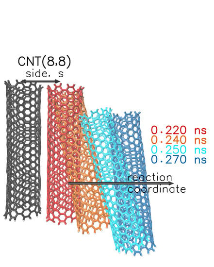
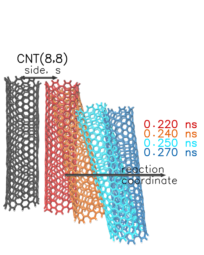
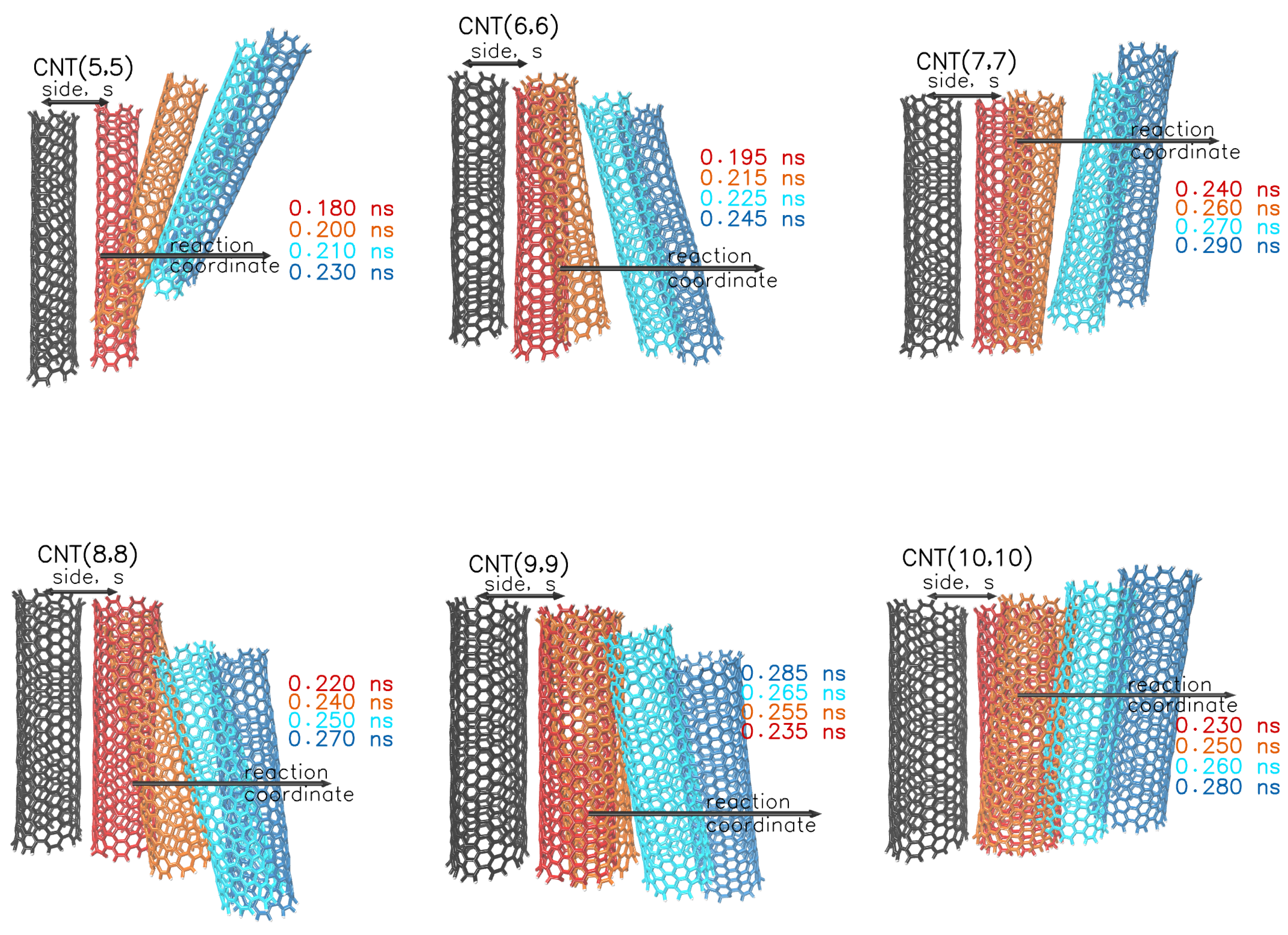
In Figure 2, we present a set of configurations from the pulling simulations. The left nanotube (black color) is constrained at a fixed position. The right nanotube (red) is being pulled away by applying a force at the center of mass. When the force becomes sufficient to overcome the restoring forces, the red nanotube moves towards the specified coordinate. The position and the orientation of the pulled nanotube is drawn in four consecutive time steps in a range of 0.05 ns after the moment of separation. Although the reaction coordinate and the driving force constant is the same, the nanotubes are being pulled in different pathways. The time range of the illustrated configurations is highlighted in the bottom panel of Figure 1.

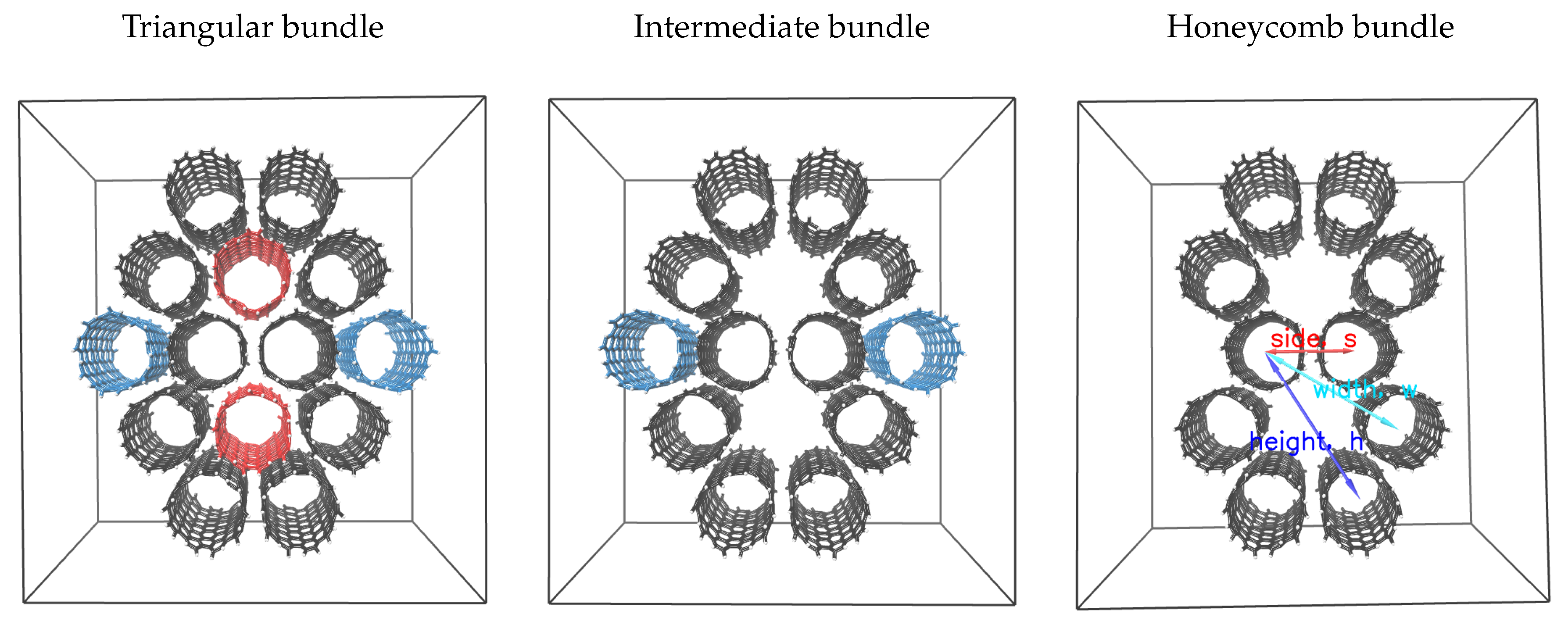
In Figure 3, we present three bundle configurations of the armchair carbon nanotube CNT(9,9). The triangular bundle corresponds to the most densely packed tiling of the nanoparticles. The intermediate bundle is configured by deleting two vertically aligned nanotubes from the triangular arrangement. The honeycomb bundle is structured by deleting two more nanotubes from the central horizontal axis of the intermediate bundle. The latter bundle consists of two hexagonal tiles of nanotubes. We use the arrows in Figure 3 to describe three critical size metrics of the bundle configurations. These are the side, s, of the adjacent nanotubes, the distance of the second closest nanotubes (width), $w=\sqrt{3}s$ and of the third closest nanotubes (height), $h=2s$, in the hexagonal tile. As noted, the side, s, is computed using pulling simulations on model duplicates of the specified structures. The width and the height are measured from the center of mass (COM) of the nanoparticles. The term, $\sqrt{3}$, comes from $sin\left({60}^{°}\right)$. In porosity measurements, it is useful to express the interparticle lengths and wall-to-wall distances. Therefore, if d is the chiral diameter of the nanotube, we use the expression $w^{\prime }=w-d$ for the width and $h^{\prime }=h-d$ for the height of the hexagonal tiles. Accordingly, the effective diameter of the nanotubes is given by $d^{\prime }=d-{\sigma }_C$, where, ${\sigma }_C$, is the Lennard Jones diameter of carbon. We list the pore size parameters of the different bundles in Table 1.

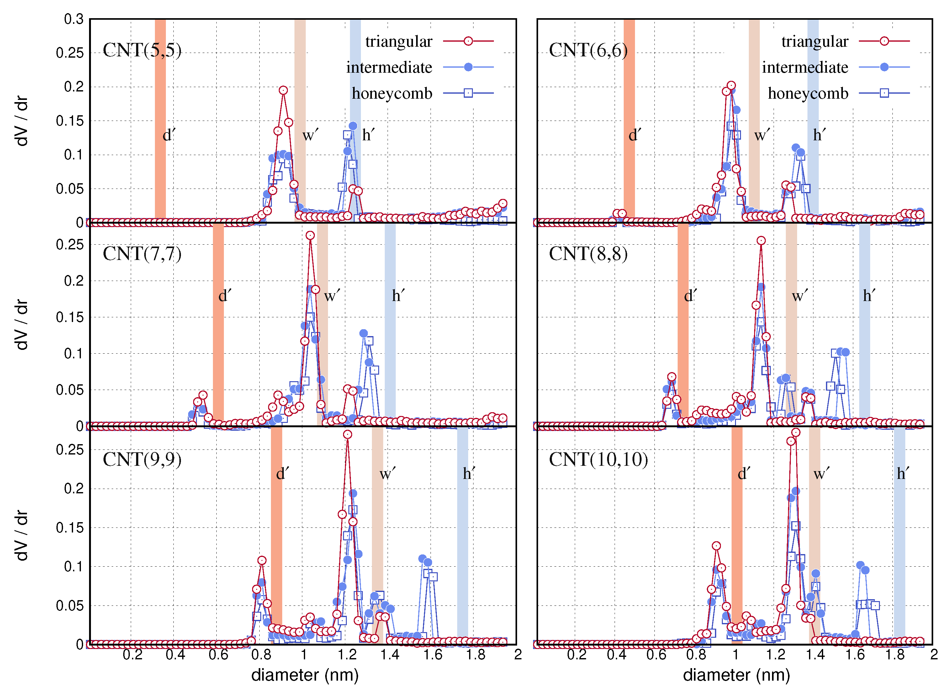
In Figure 4, we show the computed pore size distributions for the different bundles. We consider structures with triangular, intermediate and honeycomb arrangements of nanotubes. The peaks on the distributions indicate the diameter of the pores. The height of the peaks indicates the contribution of the pores to the total pore volume (TPV). We detect three distinct peaks on the distributions which correlate with some principle size metrics of the bundles. We use three coloured barriers inside the panels to spot these sizes. The sizes are the effective diameter, $d^{\prime }$, of the nanotubes, the width, $w^{\prime }$ and the height $h^{\prime }$ of the hexagonal tiles. The values are listed in Table 1. Apart from the main peaks on the distributions, other value fluctuations are due to the convex surface of the neighbouring nanotubes, which may intervene the space of $w^{\prime }$ or $h^{\prime }$ pores. The first peak of the distributions is related to the effective diameter, $d^{\prime }$, of the nanotube. The height of the first peak increases with the chiral index of the armchair nanotube since the internal volume also increases. The distributions of CNT(5,5) do not show relevant first peak, because the effective diameter of CNT(5,5) is smaller than the size (0.4 nm) of the finite cubes we used in the grid. The second and the third peak of the distributions locate close to the sizes, $w^{\prime }$ and $h^{\prime }$ respectively. Most of the cavities in the triangular bundles have a diameter comparable to $w^{\prime }$. Deleting the nanotubes from a triangular bundle, produces configurations with more open space than the initial structure. In this regard, in intermediate and honeycomb bundles the pores with size $w^{\prime }$ are reduced in number and new cavities with size $h^{\prime }$ are configured.

We note that the distributions peak slightly more on the left than the coloured barriers. This is expected due to the vacuum simulations, which we performed after configuring the bundles. The lengths, $w^{\prime }$ and $h^{\prime }$, are computed with the nanotubes immersed in water. These variables are proportional to the side, s, so that they are affected by a possible formation of water layer between the tubes during the pulling simulations. With vacuum simulations the adjacent nanotubes may approach each other closer than s, which is depicted to the resulted distributions. The vacuum simulations change the geometric properties of the as made bundles, similar to what is experimentally anticipated when evacuating the solid or extracting the solvent from the micropores.

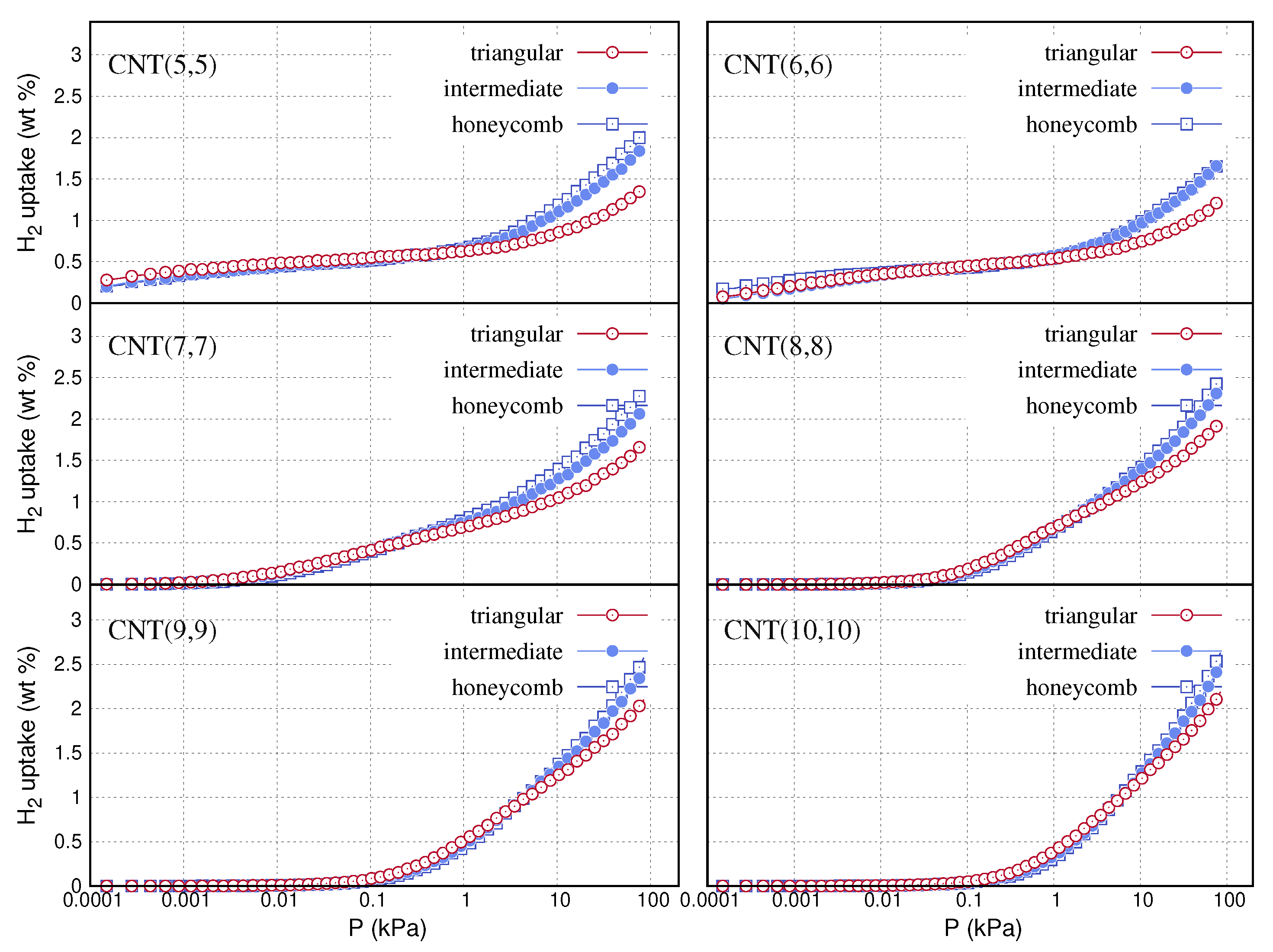
In Figure 5, we present the isotherms of hydrogen adsorption simulations on the different CNT models and bundle configurations at 77 K. The isotherms refer to the excess $H_2$ uptake using the formula for $n_{ex}$ and the total pore volume, $V_p$, of the structures, listed in

Table 2. Total pore volume (helium) of the CNT bundles arranged in triangular, intermediate and honeycomb patterns and the change (%) in respect to the pore volume of the triangular bundle.

	Total (Helium) Pore Volume (cm${}^3$/g)			Change (% from Triangular)
	Triangular	Intermediate	Honeycomb	Intermediate	Honeycomb
CNT(5,5)	1.37	1.67	2.08	22.3	52.2
CNT(6,6)	1.52	1.85	2.27	21.7	49.7
CNT(7,7)	1.50	1.80	2.21	20.1	47.5
CNY(8,8)	1.68	2.03	2.50	21.4	49.2
CNT(9,9)	1.73	2.10	2.58	21.1	48.6
CNT(10,10)	1.80	2.17	2.66	20.5	47.8

. Then we convert the output to the weight per cent, ($wt$ %) values, using the molecular weights of the bundles, $m_b$, listed in

Table 3. Molecular weight of the CNT bundles arranged in triangular, intermediate and honeycomb patterns.

	Weight (g/mol) in the Cell
	Triangular	Intermediate	Honeycomb
CNT(5,5)	23,800	20,400	17,000
CNT(6,6)	28,560	24,480	20,400
CNT(7,7)	33,320	28,560	23,800
CNT(8,8)	38,080	32,640	27,200
CNT(9,9)	42,840	36,720	30,600
CNT(10,10)	47,600	40,800	34,000

. In each panel, the three adsorption curves almost coincide at low pressures. This denotes that the different bundle arrangements of a single nanotube have similar micropore content. Hydrogen is either adsorbed inside the cavity of the nanotube or at the open space between the adjacent nanotubes. Both of these confinements are less than a few molecular diameters wide. The pore network of the CNT(5,5) and CNT(6,6) bundles consists exclusively of sub-nanometer pores. Such ultra microporous structures favour the adsorption of hydrogen at extremely low pressures. For instance, the uptake of $H_2$ in the bundles of CNT(5,5) and CNT(6,6) is ≃0.5% wt at 0.01 kPa. By increasing the diameter of the nanotube, the pore network of the bundles shifts to wider sizes. This results in the substantial decrease of $H_2$ uptake at low pressures. Near ambient pressures, hydrogen uptake is proportional to the specific surface area of the samples. The surface area values of the different bundle configurations are listed in

Table 4. Surface area of the CNT bundles arranged in triangular, intermediate and honeycomb patterns and the change (%) in respect to the surface area of the triangular bundle.

	Surface Area (m${}^2$/g)			Change (% from Triangular)
	Triangular	Intermediate	Honeycomb	Intermediate	Honeycomb
CNT(5,5)	1601.25	2081.72	2364.15	30.0	47.6
CNT(6,6)	1750.66	2221.26	2522.03	26.9	44.1
CNT(7,7)	1874.01	2291.26	2566.58	22.3	37.0
CNT(8,8)	2092.28	2609.34	2878.45	24.7	37.6
CNT(9,9)	2201.74	2679.08	2937.47	21.7	33.4
CNT(10,10)	2262.70	2760.00	3005.34	22.0	32.8

. The honeycomb and intermediate bundles have larger surface areas and adsorb greater densities than the triangular bundles. The surface area of the bundles increases with the chiral diameter of the nanotube. Accordingly, the corresponding bundle structures of the wider nanotubes adsorb greater densities at 100 kPa. In some cases, the computed hydrogen uptake at ambient pressures and 77 K may exceed 2 % wt.

Table 1. Size variables of bundle models for different armchair carbon nanotubes. The side, s, is computed with pulling simulations. The width $w^{\prime }$ and the height $h^{\prime }$ of the bundles are the wall to wall distances of the variables, w and h, shown in Figure 3.

	Diameter	Diameter (eff.)	Side	Width	Height
	$\mathit{d}$  $\left(\mathbf{nm}\right)$	${\mathit{d}}^{\prime }=\mathit{d}-{\mathit{\sigma }}_{\mathit{C}}$	$\mathit{s}$  $\left(\mathbf{nm}\right)$	${\mathit{w}}^{\prime }=\sqrt{\mathbf{3}}\mathit{s}-\mathit{d}$	${\mathit{h}}^{\prime }=\mathbf{2}\mathit{s}-\mathit{d}$
CNT(5,5)	0.678	0.338	0.963	0.991	1.249
CNT(6,6)	0.814	0.474	1.106	1.103	1.399
CNT(7,7)	0.949	0.609	1.180	1.095	1.411
CNT(8,8)	1.085	0.745	1.372	1.291	1.658
CNT(9,9)	1.221	0.881	1.485	1.352	1.750
CNT(10,10)	1.356	1.016	1.595	1.407	1.835

Table 1. Size variables of bundle models for different armchair carbon nanotubes. The side, s, is computed with pulling simulations. The width $w^{\prime }$ and the height $h^{\prime }$ of the bundles are the wall to wall distances of the variables, w and h, shown in Figure 3.

	Diameter	Diameter (eff.)	Side	Width	Height
	$\mathit{d}$  $\left(\mathbf{nm}\right)$	${\mathit{d}}^{\prime }=\mathit{d}-{\mathit{\sigma }}_{\mathit{C}}$	$\mathit{s}$  $\left(\mathbf{nm}\right)$	${\mathit{w}}^{\prime }=\sqrt{\mathbf{3}}\mathit{s}-\mathit{d}$	${\mathit{h}}^{\prime }=\mathbf{2}\mathit{s}-\mathit{d}$
CNT(5,5)	0.678	0.338	0.963	0.991	1.249
CNT(6,6)	0.814	0.474	1.106	1.103	1.399
CNT(7,7)	0.949	0.609	1.180	1.095	1.411
CNT(8,8)	1.085	0.745	1.372	1.291	1.658
CNT(9,9)	1.221	0.881	1.485	1.352	1.750
CNT(10,10)	1.356	1.016	1.595	1.407	1.835

4. Conclusions

We discuss how to produce carbon nanotube bundles in saline solution and study hydrogen adsorption properties after solvent removal and evacuation. We interplay a relatively new simulation technique, namely the pulling simulation, with an old one, the grand canonical Monte Carlo. These techniques have modules with different dependencies that we encode and execute in a single workflow. We conduct pulling simulations on pairs of nanotubes and configure high surface area bundles of such nanostructures to simulate hydrogen adsorption. We use the pull codes to compute appropriate interstitial distances for six armchair carbon nanotubes. We detect comparable puling forces and times for the nanotubes to detach. As they are being pulled, the nanotubes follow separate dissociation pathways. We measure the interstitial distances the instant before the nanotubes detach and use them as unit sizes in bundle templates. We consider three templates, each with different porous characteristics. We perform vacuum molecular dynamics on the resulted bundles which slightly change the initially set interstitial distances. All the resulted bundle structures are ultra microporous with high specific surface area. The surface area and the micropore content are crucial parameters for the materials performance for hydrogen physisorption. We simulate hydrogen adsorption on the configured bundles at 77 K. We compute and analyse the isotherms on the basis of the porosity and the chiral index of the nanotubes.

References

- Zou, C.; Zhao, Q.; Zhang, G.; Xiong, B. Energy revolution: From a fossil energy era to a new energy era. Nat. Gas Ind. 2016, 3, 1–11. [Google Scholar] [CrossRef] [Green Version]
- Ritchie, M.; Roser, M. “Energy”. Published online at OurWorldInData.org. Available online: https://ourworldindata.org/energy (accessed on 1 August 2018).
- Zhou, L. Progress and problems in hydrogen storage methods. Renew. Sustain. Energy Rev. 2005, 9, 395–408. [Google Scholar] [CrossRef]
- Zuttel, A. Materials for hydrogen storage. Mater. Today 2003, 6, 24–33. [Google Scholar] [CrossRef]
- Thomas, K.M. Hydrogen adsorption and storage on porous materials. Catal. Today 2007, 120, 389–398. [Google Scholar] [CrossRef]
- Rivard, E.; Trudeau, M.; Zaghib, K. Hydrogen Storage for Mobility: A Review. Materials 2019, 12, 1973. [Google Scholar] [CrossRef] [Green Version]
- Züttel, A.A.; Wenger, P.; Rentsch, S.; Sudan, P.; Mauron, P.H.; Emmenegger, C.H. LiBH4 a new hydrogen storage material. J. Power Sources 2003, 118, 1–7. [Google Scholar] [CrossRef]
- Sakintuna, B.; Lamari-Darkrim, F.; Hirscher, M. Metal hydride materials for solid hydrogen storage: A review. Int. J. Hydrogen Energy 2007, 32, 1121–1140. [Google Scholar] [CrossRef]
- Hirscher, M.; Yartys, V.A.; Baricco, M.; Bellosta von Colbe, J.; Blanchard, D.; Bowman, R.C.; Broom, D.P.; Buckley, C.E.; Chang, F.; Chen, P.; et al. Materials for hydrogen-based energy storage—Past, recent progress and future outlook. J. Alloy. Compd. 2019, 827, 153548. [Google Scholar] [CrossRef]
- Sherif, S.A.; Zeytinoglu, N.; Veziroglu, T.N. Liquid hydrogen: Potential, problems and a proposed research program. Int. J. Hydrogen Energy 1997, 22, 683–688. [Google Scholar] [CrossRef]
- Felderhoff, M.; Weidenthaler, C.; von Helmolt, R.; Eberle, U. Hydrogen storage: The remaining scientific and technological challenges. Phys. Chem. Chem. Phys. 2007, 9, 2643–2653. [Google Scholar] [CrossRef] [PubMed]
- Broom, D.P. Hydrogen storage materials. In The Characterisation of Their Storage Properties; Springer: London, UK, 2011; ISBN 9780857292116. [Google Scholar]
- Becher, M.; Haluska, M.; Hirscher, M.; Quintel, A.; Skakalova, V.; Dettlaff-Weglikovska, U.; Chen, X.; Hulman, M.; Choi, Y.; Roth, S.; et al. Hydrogen storage in carbon nanotubes. C. R. Phys. 2003, 4, 1055–1062. [Google Scholar] [CrossRef]
- Petrushenko, I.K.; Petrushenko, K.B. Physical adsorption of hydrogen molecules on single-walled carbon nanotubes and carbon-boron-nitrogen heteronanotubes: A comparative DFT study. Vacuum 2019, 167, 280–286. [Google Scholar] [CrossRef]
- Feng, Y.; Wang, J.; Liu, Y.; Zheng, Q. Adsorption equilibrium of hydrogen adsorption on activated carbon, multi-walled carbon nanotubes and graphene sheets. Cryogenics 2019, 101, 36–42. [Google Scholar] [CrossRef]
- Kovalev, V.; Yakunchikov, A.; Li, F. pH-sensitive loading/releasing of doxorubicin using single-walled carbon nanotube and multi-walled carbon nanotube: A molecular dynamics study. Acta Astronaut. 2011, 68, 681–685. [Google Scholar] [CrossRef]
- Brzhezinskaya, M.; Belenkov, E.A.; Greshnyakov, V.A.; Yalovega, G.E.; Bashkin, I.O. New aspects in the study of carbon-hydrogen interaction in hydrogenated carbon nanotubes for energy storage applications. J. Alloy. Compd. 2019, 792, 713–720. [Google Scholar] [CrossRef]
- Dündar-Tekkaya, E.; Karatepe, N. Hydrogen adsorption of carbon nanotubes grown on different catalysts. Int. J. Hydrogen Energy 2015, 40, 7665–7670. [Google Scholar] [CrossRef]
- Gromov, S.V.; Burmistrov, I.N.; Ilinykh, I.A.; Kuznetsov, D.V. Simulation of hydrogen adsorption on carbon nanotubes with different chirality parameters. IOP Conf. Ser. Mater. Sci. Eng. 2016, 112, 12006. [Google Scholar] [CrossRef] [Green Version]
- Maleki, R.; Afrouzi, H.H.; Hosseini, M.; Toghraie, D.; Piranfar, A.; Rostami, S. Simulation of hydrogen adsorption in carbon nanotube arrays. Comput. Methods Programs Biomed. 2020, 186, 105210. [Google Scholar] [CrossRef]
- Shkolin, A.V.; Fomkin, A.A.; Yakovlev, V.Y.; Men’shchikov, I.E. Model Nanoporous Supramolecular Structures Based on Carbon Nanotubes and Hydrocarbons for Methane and Hydrogen Adsorption. Colloid J. 2018, 80, 739–750. [Google Scholar] [CrossRef]
- Varshoy, S.; Khoshnevisan, B.; Mohsen Behpour, M. Enhanced hydrogen storage capacity of Ni/Sn-coated MWCNT nanocomposites. Nanotechnology 2018, 29, 075402. [Google Scholar] [CrossRef]
- Yang, H.; Lombardo, L.; Luo, W.; Kim, W.; Züttel, A. Hydrogen storage properties of various carbon supported NaBH4 prepared via metathesis. Int. J. Hydrogen Energy 2018, 43, 7108–7116. [Google Scholar] [CrossRef]
- Narjes, D.; Heidar, R.; Zohre, H.; Farzaneh, F. Using molecular dynamics simulation to explore the binding of the three potent anticancer drugs sorafenib, streptozotocin, and sunitinib to functionalized carbon nanotubes. J. Mol. Model. 2019, 25, 159. [Google Scholar]
- Tian, M.; Rochat, S.; Polak-Kraśna, K.; Holyfield, L.T.; Burrows, A.D.; Bowen, C.R.; Mays, T.J. Nanoporous polymer-based composites for enhanced hydrogen storage. Adsorption 2019, 25, 889–901. [Google Scholar] [CrossRef] [Green Version]
- Gao, Y.; Mao, D.; Wu, J.; Wang, X.; Wang, Z.; Zhou, G.; Chen, L.; Chen, J.; Zeng, S. Carbon Nanotubes Translocation through a Lipid Membrane and Transporting Small Hydrophobic and Hydrophilic Molecules. Appl. Sci. 2019, 9, 4271. [Google Scholar] [CrossRef] [Green Version]
- Zhan, S.; Ahlquist, M.S. Dynamics and Reactions of Molecular Ru Catalysts at Carbon Nanotube–Water Interfaces. J. Am. Chem. Soc. 2018, 140, 7498–7503. [Google Scholar] [CrossRef]
- Gusain, R.; Kumar, N.; Ray, S.S. Recent advances in carbon nanomaterial-based adsorbents for water purification. Coord. Chem. Rev. 2020, 405, 213111. [Google Scholar] [CrossRef]
- Cracknell, R.F. Simulation of hydrogen adsorption in carbon nanotubes. Mol. Phys. 2002, 100, 2079–2086. [Google Scholar] [CrossRef]
- Darkrim, F.; Levesque, D. High Adsorptive Property of Opened Carbon Nanotubes at 77 K. J. Phys. Chem. 2000, 104, 6773–6776. [Google Scholar] [CrossRef]
- Stan, G.; Cole, M.W. Hydrogen Adsorption in Nanotubes. J. Low Temp. Phys. 1998, 110, 539–544. [Google Scholar] [CrossRef]
- Gotzias, A.; Heiberg-Andersen, H.; Kainourgiakis, M.; Steriotis, T. Grand canonical Monte Carlo simulations of hydrogen adsorption in carbon cones. Appl. Surf. Sci. 2010, 256, 5226–5231. [Google Scholar] [CrossRef]
- Gotzias, A.; Heiberg-Andersen, H.; Kainourgiakis, M.; Steriotis, T. A grand canonical Monte Carlo study of hydrogen adsorption in carbon nanohorns and nanocones at 77K. Carbon 2011, 49, 2715–2724. [Google Scholar] [CrossRef]
- Lemkul, J.A.; Bevan, D.R. Assessing the Stability of Alzheimer’s Amyloid Protofibrils Using Molecular Dynamics. J. Phys. Chem. B 2010, 114, 1652–1660. [Google Scholar] [CrossRef]
- Vijayaraj, R.; Van Damme, S.; Bultinck, P.; Subramanian, V. Molecular Dynamics and Umbrella Sampling Study of Stabilizing Factors in Cyclic Peptide-Based Nanotubes. J. Phys. Chem. B 2012, 116, 9922–9933. [Google Scholar] [CrossRef]
- Nawrocki, G.; Cieplak, M. Amino acids and proteins at ZnO–water interfaces in molecular dynamics simulations. Phys. Chem. Chem. Phys. 2013, 15, 13628–13636. [Google Scholar] [CrossRef] [Green Version]
- Gladich, I.; Habartová, A.; Roeselová, M. Adsorption, Mobility, and Self-Association of Naphthalene and 1-Methylnaphthalene at the Water–Vapor Interface. J. Phys. Chem. A 2018, 118, 1052–1066. [Google Scholar] [CrossRef]
- Hedger, G.; Shorthouse, D.; Koldsø, H.; Sansom, M. Free Energy Landscape of Lipid Interactions with Regulatory Binding Sites on the Transmembrane Domain of the EGF Receptor. J. Phys. Chem. B 2016, 120, 8154–8163. [Google Scholar] [CrossRef]
- Kolman, K.; Abbas, Z. Molecular dynamics exploration for the adsorption of benzoic acid derivatives on charged silica surfaces. Colloids Surf. Physicochem. Eng. Asp. 2019, 578, 123635. [Google Scholar] [CrossRef]
- Chakraborty, S.; Lim, F.C.; Ye, J. Achieving an Optimal Tg Change by Elucidating the Polymer–Nanoparticle Interface: A Molecular Dynamics Simulation Study of the Poly(vinyl alcohol)–Silica Nanocomposite System. J. Phys. Chem. C 2019, 123, 23995–24006. [Google Scholar] [CrossRef]
- Yan, H.; Yuan, S. Molecular Dynamics Simulation of the Oil Detachment Process within Silica Nanopores. J. Phys. Chem. C 2016, 120, 2667–2674. [Google Scholar] [CrossRef]
- Zhou, H.; Yu, H.; Zhao, X.; Yang, L.; Huang, X. Molecular dynamics simulations investigate the pathway of substrate entry active site of rhomboid protease. J. Biomol. Struct. Dyn. 2019, 37, 3445–3455. [Google Scholar] [CrossRef]
- Karozis, S.; Mavroudakis, E.; Charalambopoulou, G.; Kainourgiakis, M. Molecular simulations of self-assembled ceramide bilayers: Comparison of structural and barrier properties. Mol. Simul. 2020, 46, 1–9. [Google Scholar] [CrossRef]
- Bodnarchuk, M.S.; Dini, D.; Heyes, D.M.; Breakspear, A.; Chahine, S. Molecular Dynamics Studies of Overbased Detergents on a Water Surface. Langmuir 2017, 33, 7263–7270. [Google Scholar] [CrossRef] [Green Version]
- Huang, S.; Croy, A.; Bezugly, V.; Cuniberti, G. Molecular Dynamics Studies of Overbased Detergents on a Water Surface. Phys. Chem. Chem. Phys. 2019, 21, 24007–24016. [Google Scholar] [CrossRef] [Green Version]
- Shaoqi, Z.; De Triviño, G.; Angel, J.; Mårten, A. The Carboxylate Ligand as an Oxide Relay in Catalytic Water Oxidation. J. Am. Chem. Soc. 2019, 21, 10247–10252. [Google Scholar]
- Farrokhpour, H.; Mansouri, A.; Rajabi, A.R.; Chermahini, A.N. The effect of the diameter of cyclic peptide nanotube on its chirality discrimination. J. Biomol. Struct. Dyn. 2019, 37, 691–701. [Google Scholar] [CrossRef]
- Vijayakumar, V.; Vijayaraj, R.; Peters, G.H. In silico study of amphiphilic nanotubes based on cyclic peptides in polar and non-polar solvent. J. Mol. Model. 2016, 22, 264. [Google Scholar] [CrossRef]
- Minoia, A.; Guo, Z.; Xu, H.; George, S.J.; Schenning, A.; Feyter, S.; Lazzaroni, R. Assessing the role of chirality in the formation of rosette-like supramolecular assemblies on surfaces. Chem. Commun. 2011, 47, 10924–10926. [Google Scholar] [CrossRef]
- Jorgensen, W.L.; Maxwell, D.S.; Tirado-Rives, J. Development and Testing of the OPLS All-Atom Force Field on Conformational Energetics and Properties of Organic Liquids. J. Am. Chem. Soc. 1996, 118, 11225–11236. [Google Scholar] [CrossRef]
- Abraham, M.J.; Murtola, T.; Schulz, R.; Páll, S.; Smith, J.C.; Hess, B.; Lindahl, E. GROMACS: High performance molecular simulations through multi-level parallelism from laptops to supercomputers. SoftwareX 2015, 1–2, 19–25. [Google Scholar] [CrossRef] [Green Version]
- Gotzias, A.; Kouvelos, E.; Sapalidis, A. Computing the temperature dependence of adsorption selectivity in porous solids. Surf. Coat. Technol. 2018, 350, 95–100. [Google Scholar] [CrossRef]
- Gotzias, A. Calculating adsorption isotherms using Lennard Jones particle density distributions. J. Phys. Condens. Matter 2019, 31, 435901. [Google Scholar] [CrossRef] [PubMed]
- Düren, T.; Millange, F.; Férey, G.; Walton, K.S.; Snurr, R.Q. Calculating Geometric Surface Areas as a Characterization Tool for Metal Organic Frameworks. J. Phys. Chem. C 2007, 111, 15350–15356. [Google Scholar] [CrossRef]
- Sarkisov, L.; Harrison, A. Computational structure characterisation tools in application to ordered and disordered porous materials. Mol. Simul. 2011, 37, 1248–1257. [Google Scholar] [CrossRef]
- Miklitz, M.; Jelfs, K. pywindow: Automated Structural Analysis of Molecular Pores. J. Chem. Inf. Model. 2018, 58, 2387–2391. [Google Scholar] [CrossRef]
- Lacomi, P.; Llewellyn, P. pyGAPS: A Python-based framework for adsorption isotherm processing and material characterisation. Adsorption 2019, 25, 1533–1542. [Google Scholar]
- Frenkel, D.; Smit, B. Understanding Molecular Simulation: From Algorithms to Applications; Academic: New York, NY, USA, 1996. [Google Scholar]
- Cousins, K.; Zhang, R. Highly Porous Organic Polymers for Hydrogen Fuel Storage. Polymers 2019, 11, 690. [Google Scholar] [CrossRef] [Green Version]
- Tanaka, H.; Kanoh, H.; Yudasaka, M.; Iijima, S.; Kaneko, K. Quantum Effects on Hydrogen Isotope Adsorption on Single-Wall Carbon Nanohorns. J. Am. Chem. Soc. 2005, 127, 7511–7516. [Google Scholar] [CrossRef]
- Gotzias, A.; Steriotis, T. D2/H2 quantum sieving in microporous carbons: A theoretical study on the effects of pore size and pressure. Mol. Phys. 2012, 110, 1179–1187. [Google Scholar] [CrossRef]
- Gotzias, A.; Charalambopoulou, G.; Ampoumogli, A.; Krkljus, I.; Hirscher, M.; Steriotis, T. Experimental and theoretical study of D2/H2 quantum sieving in a carbon molecular sieve. Adsorption 2013, 19, 373–379. [Google Scholar] [CrossRef]
- Krkljus, I.; Steriotis, T.; Charalambopoulou, G.; Gotzias, A.; Hirscher, M. H2/D2 adsorption and desorption studies on carbon molecular sieves with different pore structures. Carbon 2013, 57, 239–247. [Google Scholar] [CrossRef]
Figure 1.
Force and distance versus time of pulling simulations on duplicate models of armchair nanotubes with chiral index from to . The highlighted time range at the bottom panel corresponds to the time range of the snapshot configurations presented in Figure 2.
Figure 2.
Pathways of pulled nanotubes at four consecutive time steps, after the separation point (red). The reference (immobile) nanotube is coloured in black.The pulled nanotube is coloured differently (red, orange, cyan, and blue) as the distance increases. The long arrow indicates the reaction coordinate. The double arrow above the reference and the pulled nanotubes (side, s) indicates the center of mass distance before the separation.
Figure 3.
Triangular, intermediate, and honeycomb bundles of CNT(9,9). The arrows in the third panel, represent the center of mass distances of the closest (side), second closest (width) and third closest (height) nanotubes of the honeycomb bundle.
Figure 4.
Pore size distributions of triangular, intermediate and honeycomb bundles of different armchair carbon nanotubes. The column bars in the panels represent the efective diameter, , of the nanotubes, the width, and the height, , of the bundle configurations. The particular values are listed in Table 1.
Figure 5.
Simulated hydrogen adsorption isotherms up to 100 kPa at 77 K, for the triangular intermediate and honeycomb bundle models of the armchair carbon nanotubes, CNT(n,n).