Article

Fast Fourier-Based Phase Unwrapping on the Graphics Processing Unit in Real-Time Imaging Applications

1
Laboratory of Biomedical Physics, University of Antwerp, Groenenborgerlaan 171, B-2020 Antwerp, Belgium
2
Minds-VisionLab, Department of Physics, University of Antwerp, Universiteitsplein 1, B-2610 Wilrijk, Belgium
*
Author to whom correspondence should be addressed.
Submission received: 30 March 2015 / Accepted: 10 June 2015 / Published: 15 June 2015

Abstract

:
Numerous imaging techniques measure data that are mathematically wrapped to the finite interval [−π, π], corresponding to the principle value domain of the arctangent function. A wide range of reconstruction algorithms has been developed to obtain the true, unwrapped phase by adding an integral multiple of 2π to each point of the wrapped grid. However, the phase unwrapping procedure is hampered by the presence of noise, phase vortices or insufficiently sampled digital data. Unfortunately, reliable phase unwrapping algorithms are generally computationally intensive and their design often requires multiple iterations to reach convergence, leading to high execution times. In this paper, we present a high-speed phase unwrapping algorithm that is robust against noise and phase residues. By executing the parallel implementation of a single-step Fourier-based phase unwrapping algorithm on the graphics processing unit of a standard graphics card, we were able to reduce the total processing time of the phase unwrapping algorithm to < 5 ms when executed on a 640 × 480-pixel input map containing an arbitrarily high density of phase jumps. In addition, we expand upon this technique by inserting the obtained solution as a preconditioner in the conjugate gradient technique. This way, phase maps that contain regions of low-quality or invalid data can be unwrapped iteratively through weighting of local phase quality.

Graphical Abstract

1. Introduction

Phase maps are generated in many applications in medicine, physics and engineering to quantify a wide variety of different physical properties. In optics, profilometric [1,2] and interferometric [3,4,5] techniques deliver phase maps to measure topological or mechanical properties such as shape, strain and local deformation of materials. Also, beyond the field of optics, phase images are generated by many imaging techniques. In magnetic resonance imaging, susceptibility-weighted phase mapping offers a new form of contrast enhancement between structures with different magnetic susceptibilities [6] and blood flow trajectories can be monitored through velocity encoded phase gradient echo imaging [7]. Remote sensing techniques that rely on synthetic aperture radar generate phase information that is used in a host of geodetic applications to monitor geodynamical phenomena such as tectonic deformation [8], volcanic activity [9] and glacial motion [10,11]. Electron holography recovers the electron phase to produce electrostatic and magnetostatic potential distribution maps of the sample [12,13] and optical holography techniques capture the phase of reflected light beams to measure relative movement or deformation [14,15] of the sample.
A common obstacle in the image processing schemes of the above techniques is the fact that the obtained phase map is defined only to within a single 2π-cycle. That is, the value of each measurement point in the phase map is generally wrapped to the region [−π, π], corresponding to the principle value domain of the arctangent function. Therefore, phase unwrapping needs to be carried out before the phase map can be linked to the actual physical property it represents. The ability to correctly extract the true phase map from the principle value of the phase is severely complicated by the presence of noise and phase vortices [16,17,18]. To this end, a lot of effort has been made to increase the robustness of the phase-unwrapping process. When the image is processed sequentially, the phase unwrapping problem is a cumulative process where the error generated by the correction for a false jump or the miss of a genuine one will propagate throughout the rest of the image. In order to avoid or at least minimize false phase jumps, a multitude of phase unwrapping algorithms have been proposed over the years, including region-growing algorithms [19], discontinuity minimization algorithms [20], minimum Lp-norm [21] and least-squares [22] algorithms, quality-guided [23,24] and network flow [25] algorithms, branch-cut [26] algorithms and flood-fill [27] algorithms. The processing times of these algorithms range from seconds to minutes, and in some cases hours to generate a standard 640 × 480-pixelphase map [28,29]. Generally, the quality of the phase unwrapping methods increases with theirexecution time [30]. This is due to their iterative nature and local multi-pixel dependency, which inhibits parallel implementation in regular coordinate space. If the produced phase map contains minimal noise and is sufficiently well sampled between consecutive phase jumps, optimized scan-line algorithms may be employed to boost the speed of quality guided algorithms [31]. However, the above-mentioned imaging techniques cannot always guarantee such conditions and applications that aspire real-time visualization of their results often find the phase unwrapping step to be the bottleneck in their image processing schemes [32].
Two state-of-the-art Fourier-based phase unwrapping techniques were described by Schofield and Zhu [33] and by Volkov and Zhu [34]. The algorithms were developed in the field of electron holography and were designed specifically for superior stability against noise and residues present in the wrapped phase map. At their core, unlike the above-mentioned algorithms, they are both single-iteration methods that employ a combination of Fourier techniques to perform phase unwrapping in reciprocal space. As integration is performed in Fourier space, the algorithms are path-independent and show good noise-resistance in real-space.
In this manuscript, we show that optimized serial implementation of this Fourier-based phase unwrapping technique results in processing times which are limited to several tens of milliseconds, depending on the size of the input phase map. As these processing speeds are insufficiently fast for many real-time imaging applications, we propose a breakthrough in speed by optimizing the phase unwrapping algorithm for execution on parallel hardware. We demonstrate that the total processing time can be reduced by over an order of magnitude when compared to serial code by offloading the algorithm to a standard commodity graphics board. This way, a common bottleneck that is currently present in many real-time imaging applications that require high-speed phase unwrapping can be eliminated. Furthermore, we show that its parallel implementation preserves the algorithm’s superior performance for noisy images or images with high phase gradients. Additionally, a similar approach will be explored to solve the phase unwrapping problem by representing the 2D wrapped phase map as a set of sparse linear equations and by optimizing the minimization procedure of the preconditioned conjugate gradient (PCG) algorithm in Fourier space. The major advantage of this approach is that it allows the user to weight the iterative PCG solver towards areas of high quality phase data and away from areas within the phase map in which noise is expected to corrupt the phase unwrapping procedure. By providing the algorithm with a local quality map that quantifies pixel validity, convergence of the minimization procedure can be accelerated.

2. Method and Implementation

2.1. Schofield, Volkov and Zhu Phase Unwrapping

The general problem of phase unwrapping boils down to the correct extraction of the true phase φ ( r ) from the wrapped phase φ W ( r ) by constructing an integer number field k ( r ) such that (1) becomes an identity for all r N :
φ ( r ) = φ W ( r ) + 2 π k ( r )
Although both methods developed by Volkov and Zhu and Schofield and Zhu aim to solve (1) using a set of Fourier techniques, their specific implementations differ. Whereas the Volkov algorithm combines the use of several Fourier transform properties with the symmetrization rule [35] to obtain, in one go, the whole field of integer numbers k ( r ) , the Schofield algorithm formulates (1) in terms of Laplace operators:
k ( r ) = 1 2 π 2 [ 2 φ ( r ) 2 φ W ( r ) ]
where 2 and 2 represent the forward and inverse 2-dimensional Laplace operators, respectively. Next, Equation (2) can be solved using fast Fourier techniques for the Laplacians [36]:
2 f ( x , y ) = 4 π 2 M N I D C T { ( p 2 + q 2 ) D C T [ f ( x , y ) ] }
2 g ( x , y ) = M N 4 π 2 I D C T { D C T [ g ( x , y ) ] ( p 2 + q 2 ) }
given an M × N -pixel sized image with ( x , y ) its real space and ( p , q ) its Fourier space pixel coordinates. By using discrete cosine transforms (DCT) and inverse discrete cosine transforms (IDCT) instead of general fast Fourier transforms (FFT) [37], the Neumann boundary conditions that require the gradient of k ( r ) normal to the original image boundary to vanish is met and the additional memory transfers required by the symmetrization rule can be avoided. As it is our goal to achieve fast execution of the algorithm on parallel hardware, it is best to avoid as many additional memory transfers as possible. Therefore, the design principle of the Schofield algorithm was chosen for further parallel implementation. In order to solve (2) without prior knowledge of the true unwrapped phase φ ( r ) , the authors define the complex quantity P ( r ) = e x p [ i φ W ( r ) ] =   e x p [ i φ ( r ) i 2 π k ( r ) ] = e x p [ i φ ( r ) ] and recognize that I m ( ( 1 / P ) 2 P ) = 2 φ [38], where I m ( ) indicates the imaginary part. The combination of these identities yields an expression for the Laplacian of the unwrapped phase, using only knowledge of the wrapped phase:
2 φ = cos φ W 2 ( sin φ W ) sin φ W 2 ( cos φ W )
Combining Equations (3–5) along with enforcing the constraint that k ( r ) must be an integer number results in a single-step solution for Equation (2) and ultimately in a fast and deterministic solution for Equation (1).

2.2. Preconditioned Conjugate Gradient Phase Unwrapping

The Schofield, Volkov and Zhu phase unwrapping technique implicitly requires correct phase data information to be present across the entire wrapped phase map. In many practical applications, this is not the case. For such applications, input data weighting based on user-defined quality masks may be desirable. To this end, we propose to employ the approximate solution obtained with the Schofield, Volkov and Zhu technique as a first estimator of the unwrapped phase and iteratively weigh the obtained solution using a preconditioned conjugate gradient algorithm. The PCG method of 2D-weighted least-squares phase unwrapping is presented in detail in numerous papers [39,40,41,42]. For a thorough treatment of conjugate gradient methods, the reader is referred to Kershaw et al. [43]. First, an approximate solution is obtained using Equations (1–5). This solution is then used as a preconditioned input to an iterative solver which converges towards the exact solution in N or less iterations for an N × N problem. However, in practice, the preconditioning step greatly increases convergence speed so that the problem may be solved sufficiently well in only a few iterations.
In essence, the weighted PCG algorithm requires iterative minimization of:
ε 2 = i = 0 M 2 j = 0 N 2 ( φ i + 1 , j φ i , j Δ i , j x ) 2 + i = 0 M 2 j = 0 N 2 ( φ i + 1 , j φ i , j Δ i , j y ) 2
where φ i , j is the discrete wrapped phase value at coordinate point ( i , j ) and Δ i , j x and Δ i , j y represent the phase differences of the unwrapped phase grid in the x- and y-direction, respectively. This minimization problem can be solved iteratively, as shown in the pseudo-code below:
f o r   k = 0 M a x   I t e r a t i o n s A p p l y   p r e c o n d i t i o n i n g   s t e p   ( E q u a t i o n s   ( 1 5 ) ) U p d a t e   s o l u t i o n   u s i n g   w e i g h t e d   c o n j u g a t e   g r a d i e n t   m e t h o d C h e c k   f o r   c o n v e r g e n c e    i f   C o n v e r g e n c e   t h e n     E x i t   l o o p    e n d   i f e n d   f o r
The weighted conjugate gradient method allows the user to influence the relative importance of different phase values in coordinate space by amplifying or reducing their discrete contribution to the total sum of ε 2 .

2.3. Parallel Implementation of the Discrete Cosine Transform

In order to prepare the algorithm for optimized execution on parallel hardware, we write the discrete cosine transform as a combination of matrix multiplications. As the DCT is a separable linear transformation, the two-dimensional variant is equivalent to a one-dimensional DCT performed along the first dimension, followed by a one-dimensional DCT along the second dimension. Hence, the two-dimensional DCT and corresponding IDCT for an M × N input image A and output image B can be defined as [44]:
D C T ( A ) p , q = B p , q   = α p α q m = 0 M 1 n = 0 N 1 A m , n cos p π ( 2 m + 1 ) 2 M cos q π ( 2 n + 1 ) 2 N
I D C T ( B ) m , n = A m , n   = p = 0 M 1 q = 0 N 1 α p α q B p , q cos p π ( 2 m + 1 ) 2 M cos q π ( 2 n + 1 ) 2 N
with
{ 0 p M 1 0 q N 1  and  { 0 m M 1 0 n N 1
where the normalization factors α p and α q are defined as:
α p = { 1 M ,   p = 0 2 M , 1 p M 1
α q = { 1 N ,   q = 0 2 N , 1 q N 1
If A is a square matrix, the 2D-DCT can be computed as:
D C T ( A ) = T * A * T
where T represents the square matrix containing the two-dimensional forward DCT coefficients that can be obtained through orthogonalization of Equation (7) [45]. The “*” and “ ” symbols denote matrix multiplication and matrix transposition, respectively. Alternatively, when A is a non-square rectangular matrix containing M rows and N columns, a set of square transformation coefficients F L (size M × M ) and F R (size N × N ) can still be constructed from Equation (7) such that:
B = D C T ( A ) = F L * A * F R
for any M , N 0 . Likewise, the couple of transformation matrices I L (size M × M ) and I R (size N × N ) that perform the 2D inverse discrete cosine transform can be constructed from Equation (8):
I D C T ( B ) = I L * B * I R
For a succession of DCTs on matrices of any given size, the transformation matrices F L , F R , I L and I R need to be determined only once. This way, the calculation of the DCT or IDCT transform of matrix A can be reduced to two matrix multiplications (MM).

3. Numeric and Experimental Results

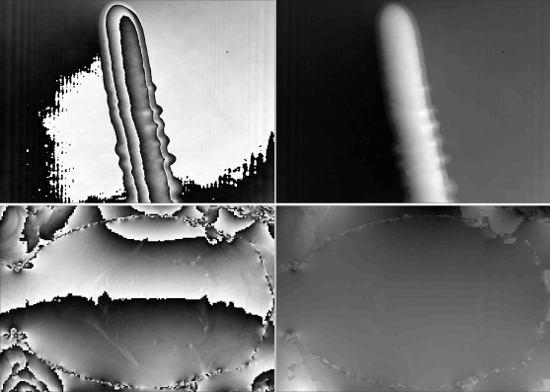
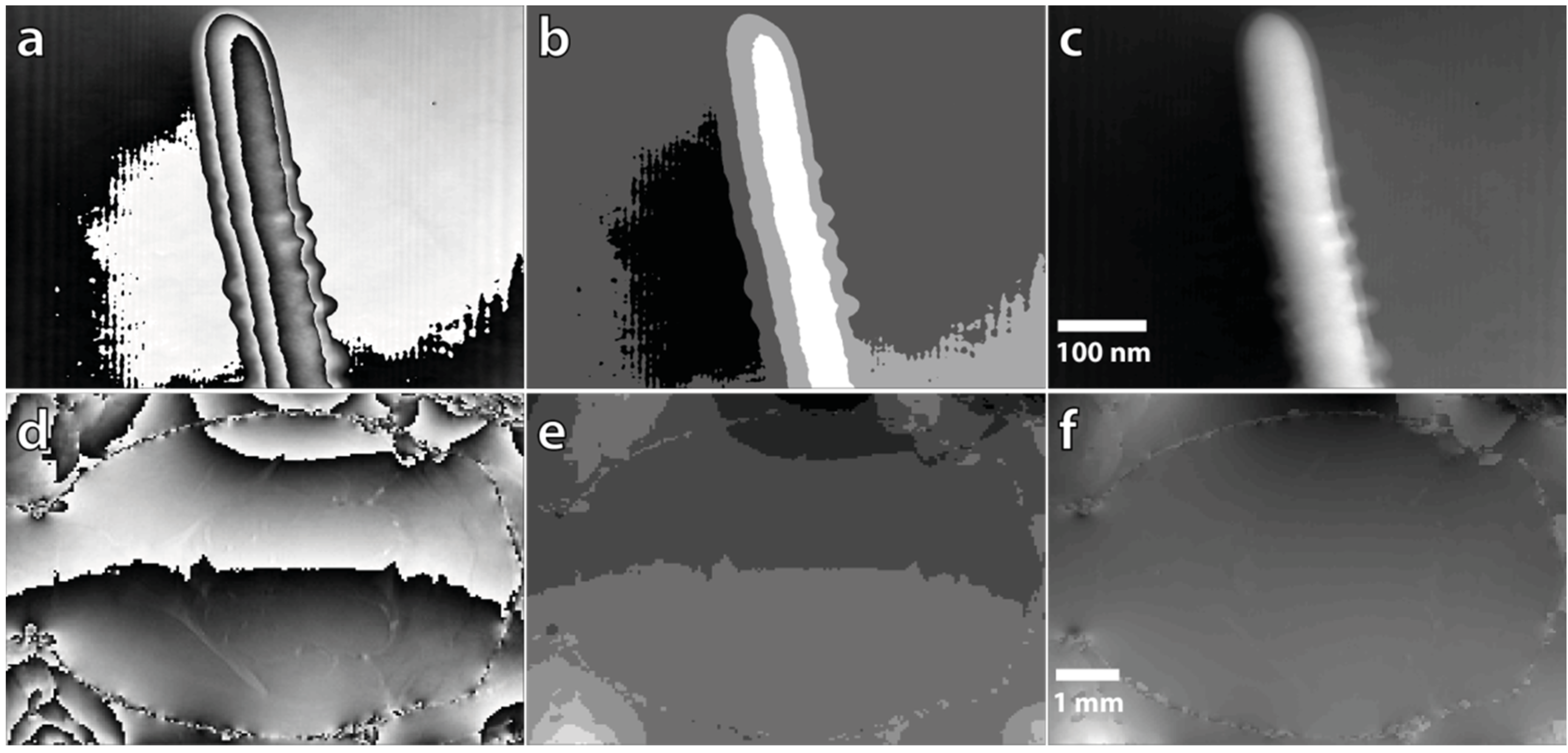
3.1. Schofield, Volkov and Zhu Phase Unwrapping

The vast majority of computational demands required by the presented phase unwrapping technique are represented by a total of six (three forward and three inverse) discrete cosine transforms. Recently, implementation optimization of the DCT on both parallel and sequential hardware has been the object of study [46,47]. Considerable speed-ups have been reported by implementing the DCT algorithm on the GPU [48,49], without loss of accuracy [50]. However, in previous work [51], it was concluded that the central processing unit (CPU) of a standard personal computer benefits most from the symmetrization rule and FFT-based DCT implementation, whereas, in contrast, the parallel architecture of the graphics processing unit (GPU) clearly favors the matrix multiplication-based approach. To this end, we have implemented the entire phase unwrapping algorithm using highly optimized CPU-code on the one hand, and in parallel code on the GPU on the other hand, each with its respective DCT implementation (CPU-FFT and GPU-MM) that results in faster execution speeds. Both CPU-and GPU-based algorithms were benchmarked on the same machine, consisting of an i5-660 processor (4MB cache, 3.33 Ghz), an NVidia Geforce GTX 770 graphics processing unit and 16 GB of RAM memory. In order to provide a fair comparison between CPU- and GPU-based versions of the presented algorithm, both were implemented using C++ code that was specifically optimized for sequential and parallel execution, respectively. The FFTW-package [52] was used to boost the calculation speed of the FFT and the Intel SSE2-instruction set was fully exploited to maximize the floating point processing capabilities of the CPU. The GPU-code was implemented using NVidia’s compute unified device architecture (CUDA) and was customized for maximum performance on all 1536 present CUDA processing cores. Furthermore, CUDA’s basic linear algebra subroutines (CUBLAS) library was used to optimize the matrix multiplications. Source code was generated and managed in Microsoft Visual Studio and its Visual Profiler with NVidia’s Nsight plug-in was used for benchmarking. Executable code can be downloaded freely at the website of the University of Antwerp [53].
The single precision (4 bytes per pixel value) execution times of both CPU-and GPU-based phase unwrapping methods were averaged over 1000 iterations of the algorithm, for a set of varying image pixel sizes. The results are included in Table 1. In addition, processing times of the isolated DCT and IDCTs, including and excluding memory transfers from host to device and back, are included in the last two columns of Table 1.
Table 1. Processing times of central processing unit (CPU)-and graphics processing unit (GPU)-based phase unwrapping algorithms, executed on phase maps of varying pixel sizes. The last two columns include the corresponding processing times of optimized GPU-accelerated discrete cosine transforms (DCTs) and inverse DCTs (IDCTs).
Image Pixel SizeCPU (FFT) (ms)GPU (MM) incl. mem. trans. (ms)GPU (MM) excl. mem. trans. (ms)Acceleration Factor (×)DCT/IDCT incl. mem trans. (ms)DCT/IDCT excl. mem trans. (ms)
256 × 2569.61.61.26.00.50.1
512 × 51240.24.13.29.81.30.3
640 × 48048.54.94.09.91.50.5
1024 × 1024182.920.116.79.15.92.5
2048 × 2048735.9136.4128.45.427.919.8
The second column of Table 1 represents the execution times of the sequential CPU-version of the entire phase unwrapping algorithm whereas the third and fourth columns indicate the corresponding processing times of the parallel GPU-based algorithm, including and excluding the memory transfers of the input image from the host to the device and back, respectively. The GPU-version of the algorithm outperforms the single-core CPU-version by a factor of 5–10 (including memory transfers). This acceleration factor increases linearly as a function of image pixel size up to input maps around 1024 × 1024 pixels where the SSE2 instruction set allows the CPU to increasingly benefit from the inherent parallelism of the single instruction, multiple data (SIMD) computations as well. Nevertheless, the GPU-over-CPU performance gains remain significant. It could be noted that further optimization of the CPU-code for execution on a multi-core CPU with an increasing number of processing cores could reduce this performance difference. However, this approach would ultimately converge to the parallel model. Furthermore, by offloading the workload of the phase unwrapping procedure to the GPU, the CPU is exempt from these calculations and can continue to coordinate other processes in the digital processing pipeline. If we benchmark the individual matrix multiplication-based DCT/IDCTs, we report processing bandwidths ranging between 131 and 204 Megapixels/s if we include the memory transfers from host to device and back. These correspond well to corresponding bandwidths of high-performance GPU-based DCTs reported in literature (141–155 Megapixels/s [48]).
In addition, the GPU processing times without memory transfers from host to device and back are included in the fourth column of Table 1 to include adequate benchmarks for phase unwrapping when the wrapped phase data is already present on GPU memory and does not need to be transferred back to host memory before visualization. As previously stated, the coefficients that are used to calculate the DCT through matrix multiplication are not included in the memory transfer time, as they need to be transferred only once, before the first iteration of the algorithm. Overall, it can be concluded that the GPU implementation of the algorithm is fast enough for most real-time applications, whereas the CPU implementation allows real-time phase unwrapping only on images of low pixel sizes and does not leave the operator with much remaining time for any additional processing.
As the success of the phase unwrapping procedure relies only on the quality of the phase map and not on the nature of the imaging technique itself, the presented algorithm can be used in a variety of applications. Figure 1 contains two such examples, one from the field of electron holography (first row), the second from magnetic resonance imaging (MRI-second row). Figure 1a contains the electrostatic and magnetostatic phase information of a Cobalt nanowire grown directly onto the grid through the use of a focused ion beam [54] and Figure 1d represents the horizontal susceptibility-weighted phase map of a mouse brain acquired with gradient echo phase-sensitive MRI [55].
Figure 1. Phase unwrapping procedure for two phase maps obtained with different imaging modalities (first row (ac): electron holography, second row (df): phase-sensitive magnetic resonance imaging (MRI)). The first column (a,d) shows the input wrapped phase map; the second column (b,e) depicts the integer number of 2π that is added to the respective wrapped phase map to end up with the unwrapped phase map, included in the third column (c,f). Scale bars are included in the third column of subfigures only but apply to the other images in their respective row, also.
Jimaging 01 00031 g001
The second column (subfigures b and e) of Figure 1 is included to emphasize the essentially deterministic quality of the presented method. It shows the k ( r ) -map of integer multiples of 2π, corresponding to the solution of (2) that need to be added to the wrapped phase images of the first column pixel-per-pixel to acquire, finally, the unwrapped phase images (subfigures c and f) of the third column of Figure 1. Although the examples contain high phase gradients, noise and phase residues, the presented method succeeds in unwrapping them correctly. It should be noted, however, that since the boundary conditions are merely approximated and a rounding step is introduced in the solution for the k ( r ) -map, the presented Fourier-based algorithm may not completely unwrap the phase map when correct phase information is not present in the entire image. For this class of images, additional iterations of the algorithm, possibly in combination with interpolation of the phase map, may be needed.

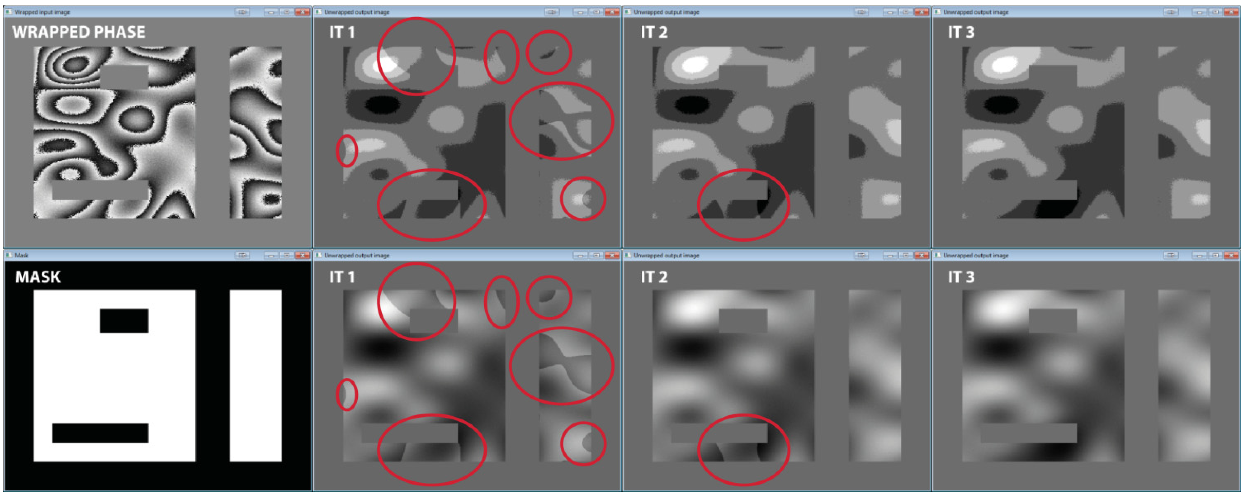
3.2. Preconditioned Conjugate Gradient Phase Unwrapping

As the Fourier-based phase unwrapping technique implicitly requires a continuous phase distribution of the original, unwrapped phase, the algorithm is known to fail on images containing regions of invalid phase information. To demonstrate this effect, a random wrapped phase map was generated containing discrete regions where phase data was deliberately set to constant zero. The failure of the algorithm can be seen in the second column of Figure 2. The integer field k ( r ) of multiples of 2π (first row) shows discontinuous jumps (circled in red) that do not correlate with the actual phase jumps, leading to incorrectly unwrapped phase maps (second row). However, by providing the PCG algorithm with an input mask of regions where we know the data is invalid (second row, first column), the approximate solution to the single-step Fourier algorithm (second row, second column) can be used as preconditioner (IT1) or first estimator in an iterative weighted conjugate gradient process. In the presented example, the minimization procedure of Equation (6) produces a correctly unwrapped phase map within two additional iterations after initial preconditioning, by weighting the intermediate solutions to the conjugate gradient method with a simple binary pixel map. The second to fourth columns of Figure 2 indicate that, in the presented example, the phase misses are reduced from seven instances (IT1) to one miss (IT2) to none (IT3).
Figure 2. The preconditioned conjugate gradient algorithm is able to correctly unwrap a randomly generated phase map containing regions where phase data is set to zero in three iterations (IT 1-3) by weighting the intermediate preconditioned conjugate gradient (PCG) solutions according to a user-defined input quality mask. Using a simple binary mask, the phase misses (circled in red) are reduced from seven to none in three iterations.
Jimaging 01 00031 g002
Construction of the preconditioner required 4.9 ms for a phase map containing 640 × 480 pixels (see Table 1), and required an additional 2.1 ms per iteration. Therefore, calculation of the third generation integer field k ( r ) in the presented example required a total processing time of 9.1 ms. This shows that the PCG-minimization procedure can be used effectively in combination with Fourier-based phase unwrapping to process input phase maps with discernible regions of invalid or corrupt data whilst still retaining real-time processing speeds. Depending on the prevalence of these regions, the user can specify a number of additional iterations which are to be calculated, at an additional processing time penalty per iteration.
Again, executable code of the preconditioned conjugate gradient-based phase unwrapping algorithm can be downloaded freely at the authors’ website [53].

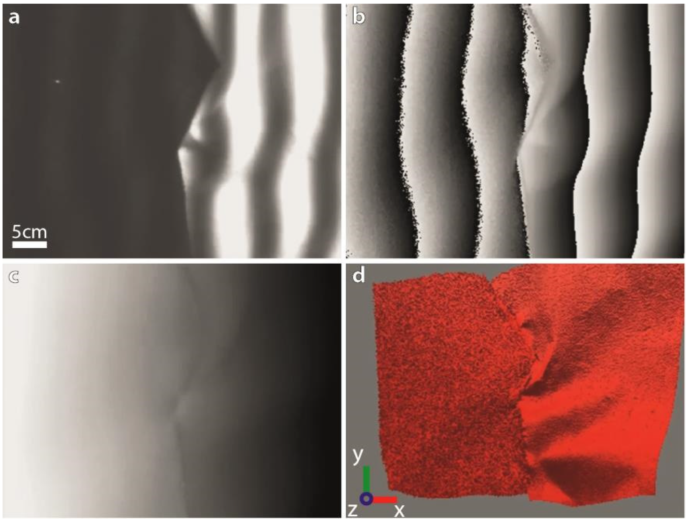
3.3. Real-Time Optical Profilometry

In order to evaluate the presented method qualitatively and to demonstrate its real-time processing capabilities, the phase unwrapping algorithm was implemented in a high-speed optical profilometry setup, similar to the one presented by Huang et al. [56]. A set of three phase-shifted line-patterns is projected onto the target at a rate of 60 projections per second. When observed by a camera with adequate frame rate, placed at an angle with the projection direction, 20 phase maps of 640 × 480 data points can be calculated from the recorded images each second. As the resulting phase values are wrapped to the finite interval [−π, π], phase unwrapping needs to take place before scaling transformations can link them to their respective height values. A single-frame excerpt from such a multi-image recording session (Media 1 [53]) is shown in Figure 3. It can be noticed that the simultaneous phase calculation, phase unwrapping procedure and multiple visualization operations can easily be completed in the provided time window of 50 ms, representing the current limit of the employed projector-camera system.
Figure 3. Single-frame excerpt from a multi-image video recording of real-time optical profilometry measurements of moving pieces of fabric (Media 1). (a) One of three phase-shifted input images. (b) Wrapped phase map. (c) Unwrapped phase map. (d) 3D perspective-view of (c).
Jimaging 01 00031 g003
To highlight the robustness of the proposed phase unwrapping algorithm, a combination of highly reflective (right side) and poorly reflective (left side) fabric was chosen as measurement object. The low amount of light reflected from the left side of the object results in a lower local contrast of observed projected line patterns, as can be seen in Figure 3a. This produces a much noisier phase distribution with less fluent phase jumps (Figure 3b), with a shadow effect at the border of both pieces of fabric. Nevertheless, the phase unwrapping algorithm is able to cope with these regions of poor phase quality perfectly as the fabric moves and shifts at reasonably high speeds. The corresponding unwrapped phase map (Figure 3c) shows no phase discontinuities throughout the recording session. An additional 3D perspective-view of (c), including vertex and fragment shading, is included in Figure 3d to allow for better depth perception of the object’s height distribution.

4. Conclusions

By combining novel Fourier-based phase unwrapping techniques with a custom parallel implementation of the two-dimensional discrete cosine transform and by optimizing its execution on the graphics processing unit of a standard low-cost graphics card, we have presented a real-time phase unwrapping algorithm that is robust in the presence of noise and phase vortices. Furthermore, its processing time is dependent only on the input pixel size and not on the phase jump density or noise level present in the image. The single-step and deterministic algorithm can unwrap the phase of input images of relatively large pixel sizes at previously unreported speeds, thereby eliminating a bottleneck that is commonly present in many applications in real-time optical profilometry and interferometry, as well as in other image processing applications in which phase map images are generated at high speeds. The parallel implementation of an iterative PCG-solver allows for additional user control over the convergence procedure of the phase unwrapping procedure.

Acknowledgments

The authors wish to thank Vyacheslav V. Volkov for sharing his insights with regard especially to the issue of specific boundary condition implementation, Elsa. Javon and Marleen Verhoye for producing the electron holography and MRI images, respectively.

Author Contributions

Sam Van der Jeught has conducted the research including parallelization and benchmarking of the code. He applied the developed algorithm to various applications and wrote the paper; Jan Sijbers and Joris J. J. Dirckx contributed to the theoretical design and development of the algorithm and aided in the writing of the paper.

Conflicts of Interest

The authors declare no conflict of interest.

References

  1. Takeda, M.; Mutoh, K. Fourier transform profilometry for the automatic measurement of 3-D object shapes. Appl. Opt. 1983, 22, 3977–3982. [Google Scholar]
  2. Srinivasan, V.; Liu, H.C.; Halioua, M. Automated phase-measuring profilometry of 3-D diffuse objects. Appl. Opt. 1984, 23, 3105–3108. [Google Scholar]
  3. Takeda, M. Spatial-carrier fringe-pattern analysis and its applications to precision interferometry and profilometry: An overview. Ind. Metrol. 1990, 1, 79–99. [Google Scholar]
  4. McDonach, A.; McKelvie, J.; McKenzie, P.; Walker, C.A. Improved moire interferometry and applications in fracture mechanics, residual stress and damaged composites. Exp. Tech. 1983, 7, 20–24. [Google Scholar]
  5. Dirckx, J.J.J.; Buytaert, J.A.N.; Van der Jeught, S. Implementation of phase-shifting moiré profilometry on a low-cost commercial data projector. Opt. Laser Eng. 2010, 48, 244–250. [Google Scholar]
  6. Haacke, E.M.; Mittal, S.; Wu, Z.; Neelavalli, J.; Cheng, Y.C. Susceptibility-weighted imaging: Technical aspects and clinical applications, part 1. Am. J. Neuroradiol. 2009, 30, 19–30. [Google Scholar] [CrossRef] [PubMed]
  7. Gatehouse, P.D.; Keegan, J.; Crowe, L.A.; Masood, S.; Mohiaddin, R.H.; Kreitner, K.F.; Firmin, D.N. Applications of phase-contrast flow and velocity imaging in cardiovascular MRI. Eur. Radiol. 2005, 15, 2172–2184. [Google Scholar]
  8. Colesanti, C.; Ferretti, A.; Prati, C.; Rocca, F. Monitoring landslides and tectonic motion with the permanent scatterers technique. Eng. Geol. 2003, 68, 3–14. [Google Scholar]
  9. Lu, Z.; Mann, D.; Freymueller, J.T.; Meyer, D.J. Synthetic aperture radar interferometry of Okmok volcano, Alaska: Radar observations. J. Geophys. Res. 2000, 105, 10791–10806. [Google Scholar]
  10. Rignot, E.; Hallet, B.; Fountain, A. Rock glacier surface motion in Beacon Valley, Antarctica, from synthetic-aperture radar interferometry. Geophys. Res. Lett. 2002, 29, 1–4. [Google Scholar]
  11. Strozzi, T.; Luckman, A.; Murray, T.; Wegmuller, U.; Werner, C.L. Glacier motion estimation using SAR offset-tracking procedures. Geosci. Remote Sens. 2002, 40, 2384–2391. [Google Scholar]
  12. Harp, G.R.; Saldin, D.K.; Tonner, B.P. Atomic-resolution electron holography in solids with localized sources. Phys. Rev. Lett. 1990, 65, 1012–1015. [Google Scholar]
  13. Tonomura, A. Applications of electron holography. Rev. Mod. Phys. 1987, 59, 639–669. [Google Scholar]
  14. Schnars, U.; Jüptner, W. Direct recording of holograms by a CCD target and numerical reconstruction. Appl. Opt. 1994, 33, 179–181. [Google Scholar]
  15. Schumann, W.; Dubas, M. Holographic Interferometry: From the Scope of Deformation Analysis of Opaque Bodies; Springer Series in Optical Sciences; Springer-Verlag: Berlin, Germany; New York, NY, USA, 1979; Volume 16. [Google Scholar]
  16. Itoh, K. Analysis of the phase unwrapping algorithm. Appl. Opt. 1982, 21, 2470. [Google Scholar]
  17. Huntley, J.M. Noise-immune phase unwrapping algorithm. Appl. Opt. 1989, 28, 3268–3270. [Google Scholar]
  18. Cusack, R.; Huntley, J.M.; Goldrein, H.T. Improved noise-immune phase-unwrapping algorithm. Appl. Opt. 1995, 34, 781–789. [Google Scholar]
  19. Xu, W.; Cumming, I. A region-growing algorithm for InSAR phase unwrapping. Geosci. Remote Sens. 1999, 37, 124–134. [Google Scholar]
  20. Flynn, T.J. Two-dimensional phase unwrapping with minimum weighted discontinuity. J. Opt. Soc. Am. A 1997, 14, 2692–2701. [Google Scholar]
  21. Ghiglia, D.C.; Romero, L.A. Minimum Lp-norm two-dimensional phase unwrapping. J. Opt. Soc. Am. A 1996, 13, 1999–2013. [Google Scholar]
  22. Pritt, M.D.; Shipman, J.S. Least-squares two-dimensional phase unwrapping using FFT’s. Geosci. Remote Sens. 1994, 32, 706–708. [Google Scholar]
  23. Herráez, M.A.; Burton, D.R.; Lalor, M.J.; Gdeisat, M.A. Fast two-dimensional phase-unwrapping algorithm based on sorting by reliability following a noncontinuous path. Appl. Opt. 2002, 41, 7437–7444. [Google Scholar]
  24. Zhong, H.; Tang, J.; Zhang, S.; Chen, M. An improved quality-guided phase-unwrapping algorithm based on priority queue. Geosci. Remote Sens. Lett. 2011, 8, 364–368. [Google Scholar]
  25. Curtis, C.W.; Zebker, H.A. Network approaches to two-dimensional phase unwrapping: Intractability and two new algorithms. J. Opt. Soc. Am. A 2000, 17, 401–414. [Google Scholar]
  26. Gutmann, B.; Weber, H. Phase unwrapping with the branch-cut method: Role of phase-field direction. Appl. Opt. 2000, 39, 4802–4816. [Google Scholar]
  27. Asundi, A.; Wensen, Z. Fast phase-unwrapping algorithm based on a gray-scale mask and flood fill. Appl. Opt. 1998, 37, 5416–5420. [Google Scholar]
  28. Ghiglia, D.C.; Pritt, M.D. Two-Dimensional Phase Unwrapping: Theory, Algorithms, and Software; Wiley: New York, NY, USA, 1998. [Google Scholar]
  29. Zhang, S. Recent progresses on real-time 3D shape measurement using digital fringe projection techniques. Opt. Lasers Eng. 2010, 48, 149–158. [Google Scholar]
  30. Judge, T.R.; Bryanston-Cross, P.J. A review of phase unwrapping techniques in fringe analysis. Opt. Laser Eng. 1994, 21, 199–239. [Google Scholar]
  31. Zhang, S.; Li, X.; Yau, S.-T. Multilevel quality-guided phase unwrapping algorithm for real-time three-dimensional shape reconstruction. Appl. Opt. 2007, 46, 50–57. [Google Scholar]
  32. Pham, H.; Ding, H.; Sobh, N.; Do, M.; Patel, S.; Popescu, G. Off-axis quantitative phase imaging processing using CUDA: Toward real-time applications. Biomed. Opt. Express 2011, 2, 1781–1793. [Google Scholar]
  33. Schofield, M.A.; Zhu, Y. Fast phase unwrapping algorithm for interferometric applications. Opt. Lett. 2003, 28, 1194–1196. [Google Scholar]
  34. Volkov, V.V.; Zhu, Y. Deterministic phase unwrapping in the presence of noise. Opt. Lett. 2003, 28, 2156–2158. [Google Scholar]
  35. Volkov, V.V.; Zhu, Y.; De Graef, M. A new symmetrized solution for phase retrieval using the transport of intensity equation. Micron 2002, 33, 411–416. [Google Scholar]
  36. Gureyev, T.E.; Nugent, K.A. Phase retrieval with the transport-of-intensity equation. II. Orthogonal series solution for nonuniform illumination. J. Opt. Soc. Am. A 1996, 13, 1670–1682. [Google Scholar]
  37. Shi, W.; Zhu, Y.; Yao, Y. Discussion about the DCT/FFT phase-unwrapping algorithm for interferometric applications. Optik 2010, 121, 1443–1449. [Google Scholar]
  38. Hÿtch, M.J.; Snoeck, E.; Kilaas, R. Quantitative measurement of displacement and strain fields from HREM micrographs. Ultramicroscopy 1998, 74, 131–146. [Google Scholar]
  39. Eisenstat, S.C. Efficient implementation of a class of preconditioned conjugate gradient methods. SIAM J. Sci. Stat. Comput. 1981, 2, 1–4. [Google Scholar]
  40. Kaufmann, G.H.; Galizzi, G.E.; Ruiz, P.D. Evaluation of a preconditioned conjugate-gradient algorithm for weighted least-squares unwrapping of digital speckle-pattern interferometry phase maps. Appl. Opt. 1998, 37, 3076–3084. [Google Scholar]
  41. Saad, Y.; Schultz, M.H. Parallel implementations of preconditioned conjugate gradient methods. In Mathematical and Computational Methods in Seismic Exploration and Reservoir Modeling; Siam: Philadelphia, PA, USA, 1985; pp. 108–127. [Google Scholar]
  42. Yang, Q.; Vogel, C.R.; Ellerbroek, B.L. Fourier domain preconditioned conjugate gradient algorithm for atmospheric tomography. Appl. Opt. 2006, 45, 5281–5293. [Google Scholar]
  43. Kershaw, D.S. The incomplete Cholesky—Conjugate gradient method for the iterative solution of systems of linear equations. J. Comput. Phys. 1978, 26, 43–65. [Google Scholar]
  44. Ghiglia, D.C.; Romero, L.A. Robust two-dimensional weighted and unweighted phase unwrapping that uses fast transforms and iterative methods. J. Opt. Soc. Am. A 1994, 11, 107–117. [Google Scholar]
  45. Gailly, J.L.; Nelson, M. The Data Compression Book; M&T Books: New York, NY, USA, 1995. [Google Scholar]
  46. Aslantas, V.; Ozer, S.; Ozturk, S. Improving the performance of DCT-based fragile watermarking using intelligent optimization algorithms. Opt. Commun. 2009, 282, 2806–2817. [Google Scholar]
  47. Chen, W.H.; Smith, C.H.; Fralick, S. A fast computational algorithm for the discrete cosine transform. IEEE Trans. Commun. 1977, 25, 1004–1009. [Google Scholar]
  48. Fang, B.; Shen, G.; Li, S.; Chen, H. Techniques for efficient DCT/IDCT implementation on generic GPU. In Proceedings of the 2005 IEEE International Symposium on Circuits and Systems, ISCAS 2005, Kobe, Japan, 23–26 May 2005; pp. 1126–1129.
  49. Ruan, J.; Han, D.D. An efficient implementation of fast DCT using CUDA. Microelectron. Comput. 2009, 8, 057. [Google Scholar]
  50. Ghetia, S.; Gajjar, N.; Gajjar, R. Implementation of 2-D discrete cosine transform on GPU. Int. J. Adv. Res. Electr. Electron. Instrum. Eng. 2013, 2, 3024–3030. [Google Scholar]
  51. Ye, P.; Shi, X.; Li, X. CUDA-Based Implementation of DCT/IDCT on GPU; University of Delaware: Newark, DE, USA, 2007. [Google Scholar]
  52. Frigo, M. A fast Fourier transform compiler. ACM Sigplan Not. 1999, 34, 169–180. [Google Scholar]
  53. Van der Jeught, S. Fast Fourier-Based Phase Unwrapping. Available online: https://www.uantwerpen.be/en/rg/bimef/downloads/fourier-based-phase-/ (accessed on 12 June 2015).
  54. Javon, E.; Gatel, C.; Masseboeuf, A.; Snoeck, E. Electron holography study of the local magnetic switching process in magnetic tunnel junctions. J. Appl. Phys. 2010, 107. [Google Scholar] [CrossRef]
  55. Bakker, C.J.; de Leeuw, H.; Vincken, K.L.; Vonken, E.J.; Hendrikse, J. Phase gradient mapping as an aid in the analysis of object-induced and system-related phase perturbations in MRI. Phys. Med. Biol. 2008, 53. [Google Scholar] [CrossRef]
  56. Huang, P.S.; Zhang, S.; Chiang, F.P. Trapezoidal phase-shifting method for three-dimensional shape measurement. Opt. Eng. 2006, 44, 123601. [Google Scholar] [CrossRef]

