
Land Cover Change Image Analysis for Assateague Island National Seashore Following Hurricane Sandy


Abstract
:
1. Introduction
2. Methods
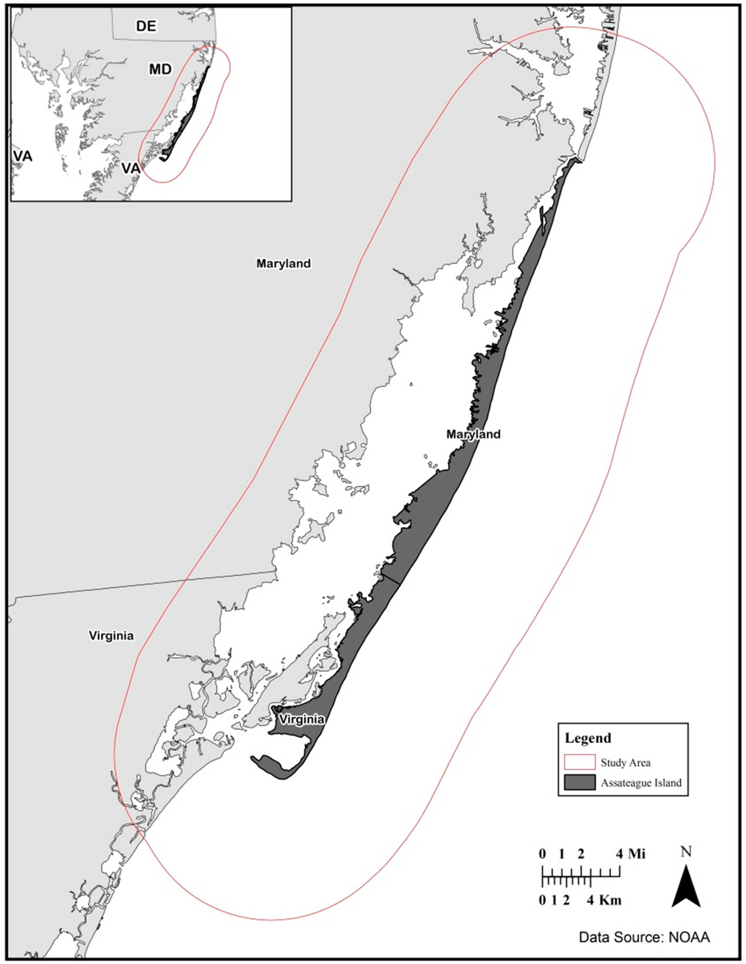
2.1. Study Area

2.2. Imagery

| Layer Stack | Sensor | Spring Image | Summer Image |
|---|---|---|---|
| Pre-Hurricane Sandy | Landsat 5 TM | 8 March 2011 | 31 August 2011 |
| Post-Hurricane Sandy | Landsat 8 OLI | 14 April 2013 | 5 September 2013 |
2.3. Image Processing
| Variable | Description |
|---|---|
| d | The sun-earth distance at time of collection |
| Lmin and Lmax | Spectral radiance calibration factors |
| DNi | The DN value at pixel i |
| DNmin | Band specific minimum DN value as determined by user |
| DNmax | Maximum possible DN value for the data ( ex. 255 for 8 bit) |
| Esun | Solar spectral irradiance |
| θz | Local solar zenith angle ( 90º- local solar elevation angle) |
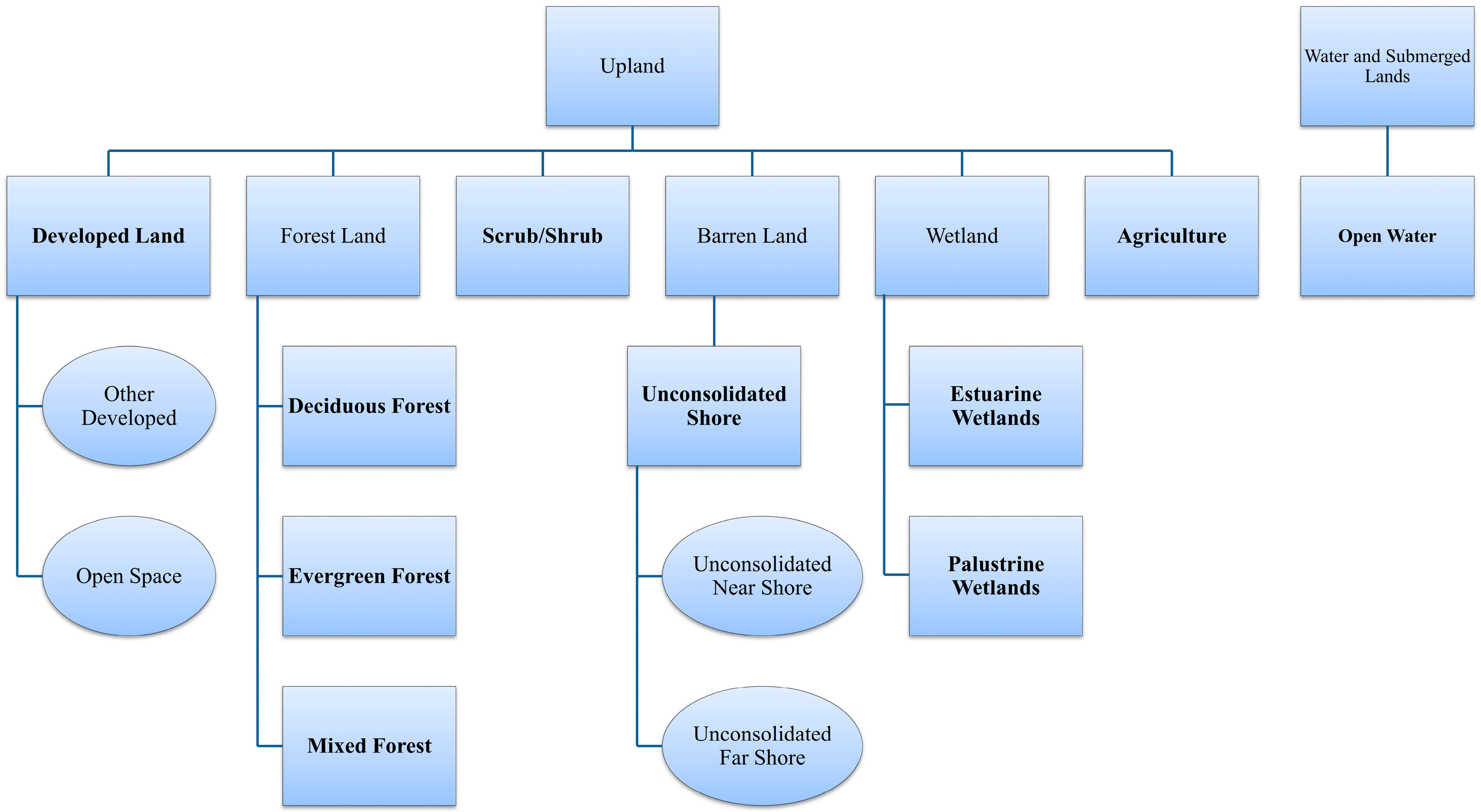
2.4. Land Cover Classification
2.4.1. Reference Data Collection

| Land Cover Class | Total Samples | Training | Accuracy |
|---|---|---|---|
| Agriculture | 106 | 53 | 53 |
| Deciduous Forest | 102 | 52 | 50 |
| Developed | 121 | 71 | 50 |
| Estuarine | 100 | 50 | 50 |
| Evergreen Forest | 100 | 50 | 50 |
| Mixed Forest | 100 | 50 | 50 |
| Open Water | 121 | 61 | 60 |
| Palustrine | 105 | 55 | 50 |
| Scrub/Shrub | 85 | 35 | 50 |
| Unconsolidated Shore | 85 | 35 | 50 |
2.4.2. Land Cover Classifications
2.4.3. Accuracy Assessment
| Spectral Feature | Spatial Features | Thematic Features |
|---|---|---|
| Mean Layer Values Standard Deviation Minimum Pixel Value Maximum Pixel Value Mean Difference to Neighbors Mean Difference To Super-Objects Ratio To Super-Objects Difference in NDVI and NLWM Difference in NIR, SWIR1, SWIR2 | Area Border Length Length Width Length/Width | Min and Maximum % overlap with the National Wetland Inventory data layer |
2.5. Land Cover Change
2.5.1. Univariate Image Differencing
2.5.2. Post Classification Comparison
3. Results
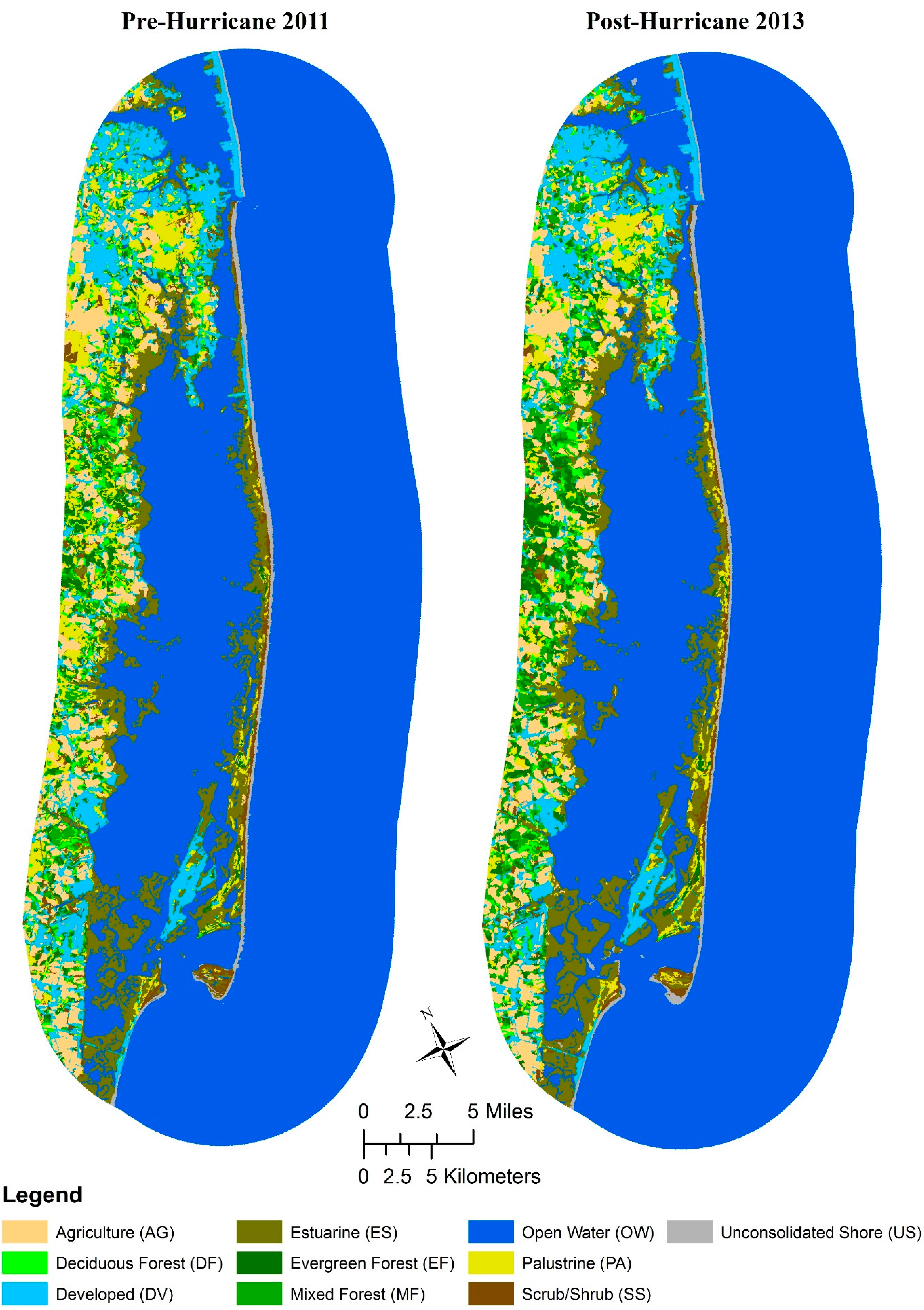
3.1. Land Cover Classification
| Band | Importance |
|---|---|
| NIR | 0.108458534 |
| SWIR 1 | 0.101598412 |
| SWIR 2 | 0.101203956 |
| Brightness | 0.099140197 |
| Greenness | 0.092806019 |
| NDVI | 0.089701816 |
| Blue | 0.083893582 |
| Red | 0.076913401 |
| Green | 0.069847479 |
| MSI | 0.066674672 |
| Wetness | 0.062730104 |
| Coastal Blue | 0.047031853 |
| Overall Accuracy | Kappa | |
|---|---|---|
| With Coastal Band | 67.57% | 0.63966 |
| Without Coastal Band | 67.57% | 0.63964 |
3.2. Accuracy Assessment
3.2.1. Single Date Classification Accuracy


| Tally-Based | Area-Based | ||||||
|---|---|---|---|---|---|---|---|
| Date | Method | Overall | Kappa | Z Statistic | Overall | Kappa | Z Statistic |
| Pre-Hurricane | Pixel | 78.90% | 0.765 | 38.325 | NA | NA | NA |
| Object | 82.64% | 0.807 | 43.255 | 89.59% | 0.874 | 144.097 | |
| Post-Hurricane | Pixel | 80.50% | 0.783 | 40.567 | NA | NA | NA |
| Object | 81.66% | 0.796 | 42.217 | 89.79% | 0.866 | 172.217 | |
| PBC | OBC | |||||
|---|---|---|---|---|---|---|
| Tally-based | Tally-based | Area-based | ||||
| UA | PA | UA | PA | UA | PA | |
| Agriculture | 100.00% | 84.00% | 97.87% | 92.00% | 98.12% | 92.08% |
| Deciduous Forest | 70.31% | 90.00% | 74.55% | 82.00% | 78.48% | 84.03% |
| Evergreen Forest | 66.67% | 84.00% | 82.22% | 74.00% | 85.65% | 79.55% |
| Mixed Forest | 72.41% | 84.00% | 82.98% | 78.00% | 82.02% | 80.94% |
| Developed | 65.75% | 96.00% | 84.21% | 96.00% | 84.29% | 98.81% |
| Open Water | 100.00% | 98.21% | 96.49% | 98.21% | 99.69% | 99.80% |
| Estuarine | 90.74% | 98.00% | 73.77% | 90.00% | 84.64% | 96.30% |
| Palustrine | 60.00% | 22.64% | 73.17% | 56.60% | 68.85% | 60.87% |
| Scrub/Shrub | 81.25% | 54.17% | 71.43% | 72.92% | 75.80% | 68.64% |
| Unconsolidated Shore | 84.78% | 78.00% | 89.58% | 86.00% | 92.08% | 85.33% |
3.2.2. Kappa Analysis
| PBC | OBC | |||||
|---|---|---|---|---|---|---|
| Land Cover Class | Tally-based | Tally-based | Area-based | |||
| UA | PA | UA | PA | UA | PA | |
| Agriculture | 90.38% | 88.68% | 89.29% | 94.34% | 91.41% | 95.31% |
| Deciduous Forest | 74.07% | 80.00% | 72.22% | 78.00% | 79.94% | 78.65% |
| Evergreen Forest | 69.09% | 76.00% | 78.26% | 72.00% | 75.64% | 76.17% |
| Mixed Forest | 73.47% | 72.00% | 64.58% | 62.00% | 66.84% | 68.51% |
| Developed | 71.93% | 82.00% | 85.45% | 94.00% | 87.88% | 97.95% |
| Open Water | 100.00% | 98.33% | 100.00% | 98.33% | 100.00% | 99.61% |
| Estuarine | 88.68% | 94.00% | 83.93% | 94.00% | 90.36% | 96.08% |
| Palustrine | 60.87% | 50.91% | 66.00% | 60.00% | 71.53% | 68.85% |
| Scrub/Shrub | 80.00% | 64.00% | 80.00% | 64.00% | 79.68% | 55.12% |
| Unconsolidated Shore | 92.45% | 98.00% | 90.74% | 98.00% | 94.44% | 99.04% |
| Method | Accuracy Assessment Type | Z Test Statistic |
|---|---|---|
| Object | Tally-based | 0.413 |
| Area-based | 0.950 | |
| Pixel | Tally-based | 0.640 |
| Classification | Z Test Statistic |
|---|---|
| Pre-Hurricane | 1.52 |
| Post-Hurricane | 1.11 |
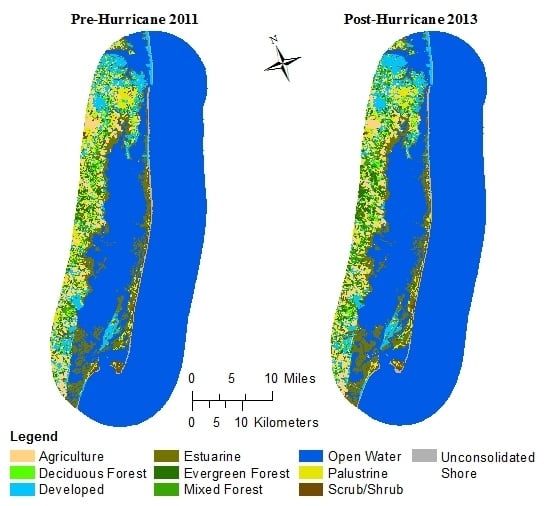
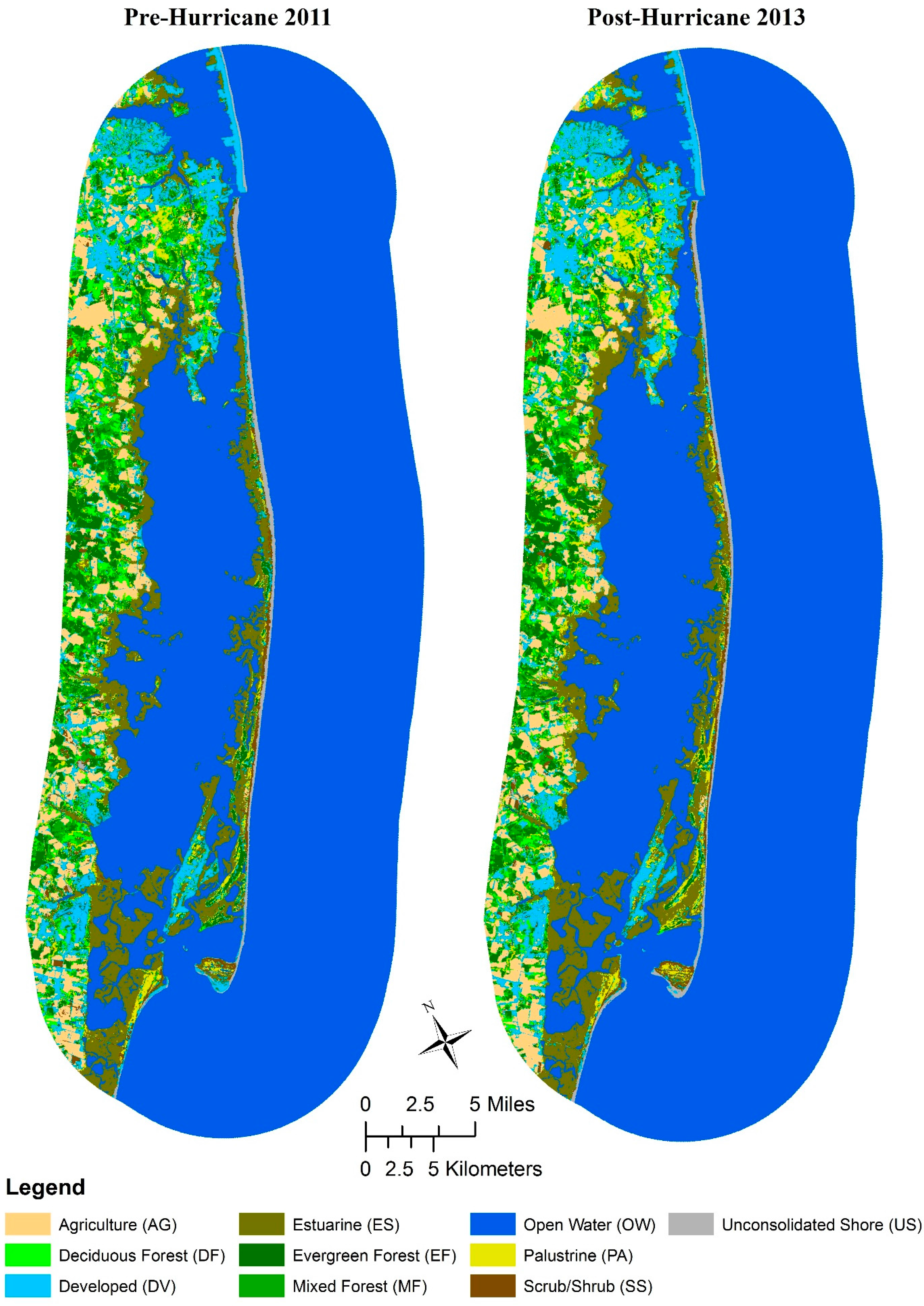
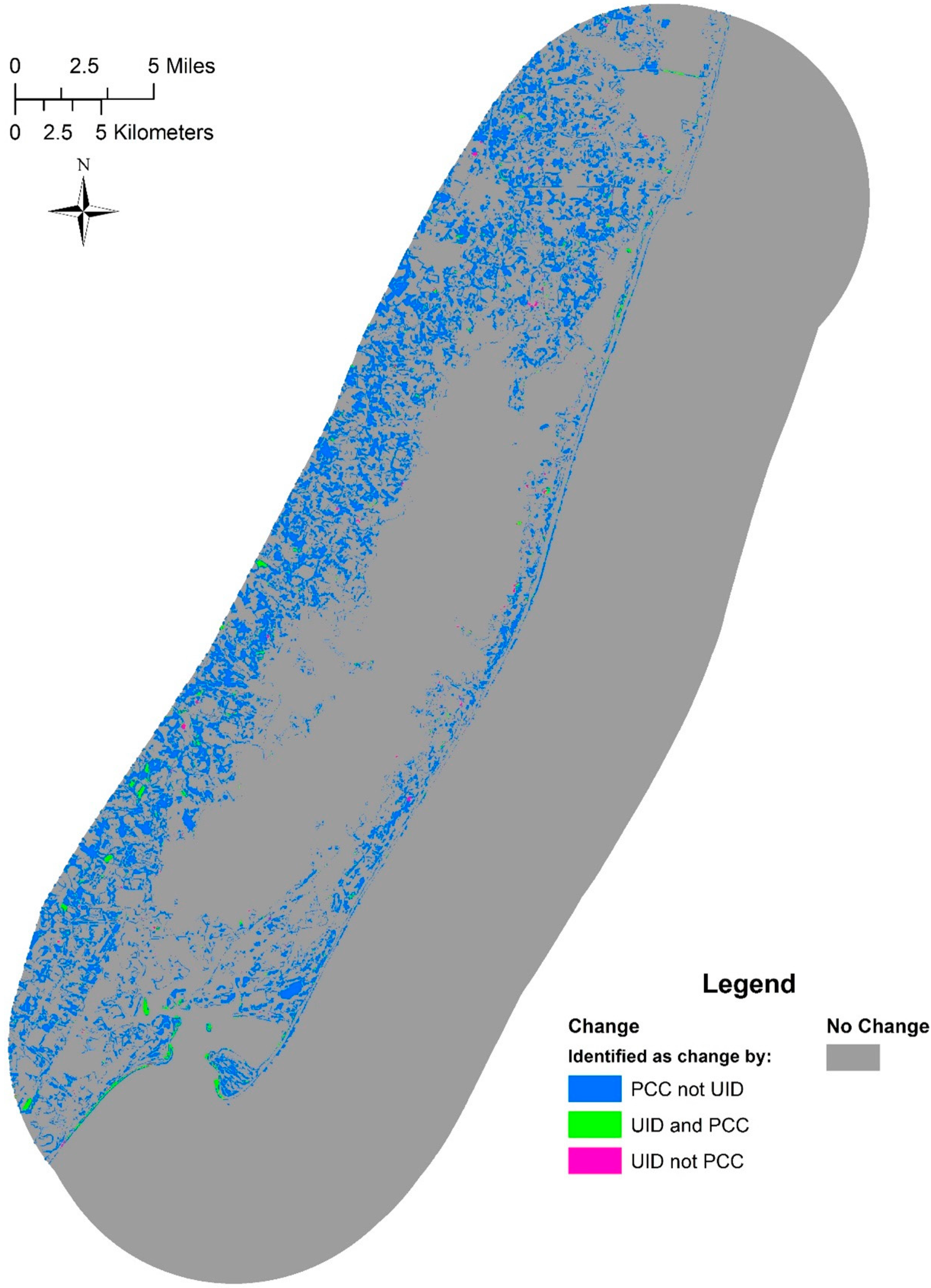
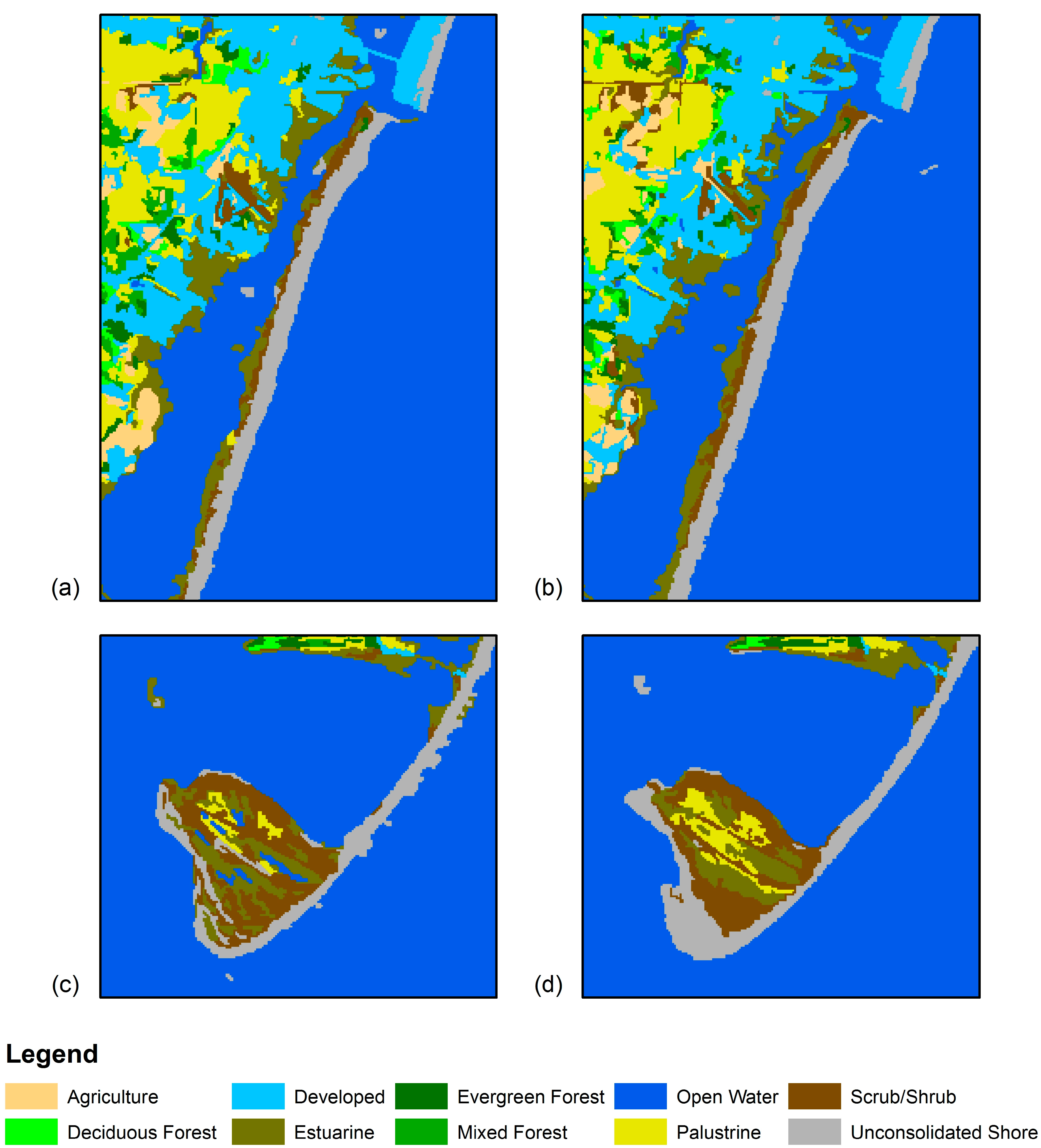
3.3. Land Cover Change Detection and Classification


| Object-Based PCC | |||
|---|---|---|---|
| Class Aggregation | Total Area Classified As Change (ha) | Percentage of Study Area Classified As Change | Percent Difference in Change Area * |
| Original Classes | 1,7149.86 | 8.98% | NA |
| Aggregate Forest Classes | 1,5030.63 | 7.87% | 12.36% |
| Aggregate Forest and Wetland Classes | 1,4151.87 | 7.41% | 17.48% |
| Pixel-Based PCC | |||
| Class Aggregation | Total Area Classified As Change (ha) | Percentage of Study Area Classified As Change | Percent Difference in Change Area * |
| Original Classes | 1,6409.16 | 8.59% | NA |
| Aggregate Forest Classes | 1,4236.65 | 7.45% | 13.24% |
| Aggregate Forest and Wetland Classes | 1,3515.3 | 7.07% | 17.64% |
| Pre-Hurricane | Post-Hurricane | Difference (ha) | Percent Change | |
|---|---|---|---|---|
| Deciduous Forest | 5.67 | 5.67 | 0.00 | 0.000% |
| Developed | 199.53 | 199.80 | 0.27 | 0.001% |
| Estuarine | 4043.71 | 3966.58 | −77.13 | 0.417% |
| Evergreen Forest | 273.24 | 274.50 | 1.26 | 0.007% |
| Open Water | 1,0457.08 | 1,0500.19 | 43.11 | 0.233% |
| Palustrine | 1040.67 | 1048.59 | 7.92 | 0.043% |
| Scrub/Shrub | 1100.70 | 1088.28 | −12.42 | 0.067% |
| Unconsolidated Shore | 1368.77 | 1405.76 | 36.99 | 0.200% |
| Total = | 0.969% |
| Pre-Hurricane | Post-Hurricane | Difference (ha) | Percent Change | ||
|---|---|---|---|---|---|
| Deciduous Forest | 6.39 | 5.67 | −0.72 | 0.004% | |
| Developed | 193.68 | 199.80 | 6.12 | 0.033% | |
| Estuarine | 4000.57 | 3966.58 | −33.99 | 0.184% | |
| Mixed Forest | 9.90 | 0.00 | −9.90 | 0.054% | |
| Evergreen Forest | 284.85 | 274.50 | −10.35 | 0.056% | |
| Open Water | 1,0644.9 | 1,0500.19 | −144.71 | 0.783% | |
| Palustrine | 674.28 | 1048.59 | 374.31 | 2.024% | |
| Scrub/Shrub | 1112.58 | 1088.28 | −24.30 | 0.131% | |
| Unconsolidated Shore | 1562.22 | 1405.76 | −156.46 | 0.846% | |
| Total = | 4.11% | ||||
4. Discussion and Conclusions
4.1. Landsat 5 vs. Landsat 8
4.2. Object vs. Pixel-Based Classification
4.3. Land Cover Change

Acknowledgments
Author Contributions
Conflicts of Interest
References
- Klemas, V.V. The role of Remote Sensing in predicting and determining coastal storm impacts. J. Coast. Res. 2009, 25, 1264–1275. [Google Scholar] [CrossRef]
- Bianchette, T.A.; Liu, K.B.; Lam, N.S.; Kiage, L.M. Ecological impacts of hurricane ivan on the gulf coast of Alabama : A remote sensing study. J. Coast. Res. 2009, 2, 1622–1626. [Google Scholar]
- Zhang, X.; Wang, Y.; Jiang, H.; Wang, X. Remote-sensing assessment of forest damage by Typhoon Saomai and its related factors at landscape scale. Int. J. Remote Sens. 2013, 34, 7874–7886. [Google Scholar] [CrossRef]
- Ramsey III, E.W.; Chappell, D.K.; Baldwin, D.G. AVHRR imagery used to identify hurricane damage in a forested wetland of Louisiana. Photogramm. Eng. Remote Sens. 1997, 63, 293–297. [Google Scholar]
- Steyer, G.D.; Couvillion, B.R.; Barras, J.A. Monitoring vegetation response to episodic disturbance events by using multitemporal vegetation indices. J. Coast. Res. 2013. [Google Scholar] [CrossRef]
- Rodgers, J.C.; Murrah, A.W.; Cooke, W.H. The impact of hurricane katrina on the coastal vegetation of the weeks bay reserve, alabama from NDVI data. Estuar. Coast. 2009, 32, 496–507. [Google Scholar] [CrossRef]
- Knutson, T.R.; McBride, J.L.; Chan, J.; Emanuel, K.; Holland, G.; Landsea, C.; Held, I.; Kossin, J.P.; Srivastava, A.K.; Sugi, M. Tropical cyclones and climate change. Nat. Geosci. 2010, 3, 157–163. [Google Scholar] [CrossRef] [Green Version]
- Webster, P.J.; Holland, G.J.; Curry, J.A.; Chang, H.-R. Changes in tropical cyclone number, duration, and intensity in a warming environment. Science 2005, 309, 1844–1846. [Google Scholar] [CrossRef] [PubMed]
- Lam, N.S.-N.; Liu, K.-B.; Liang, W.; Bianchette, T.A.; Platt, W.J. Effects of Hurricanes on the Gulf Coast ecosystems: A remote sensing study of land cover change around Weeks Bay, Alabama. J. Coast. Res. 2011, 1707–1711. [Google Scholar]
- Part A: global and sectoral aspects. contribution of working group ii to the fifth assessment report of the intergovernmental panel on climate change. In IPCC Climate Change 2014: Impacts, Adaptation, and Vulnerability; Field, C.B.; Barros, V.R.; Dokken, D.J.; Mach, K.J.; Mastrandrea, M.D.; Bilir, T.E.; Chatterjee, M.; Ebi, K.L.; Estrada, Y.O.; Genova, R.C.; et al. (Eds.) Cambridge University Press: Cambridge, United Kingdom and New York, NY, USA, 2014; pp. 361–409.
- Wang, Y.; Christiano, M.; Traber, M. Mapping salt marshes in Jamaica Bay and terrestrial vegetation in Fire Island National Seashore using QuickBird satellite data. In Remote Sensing of Coastal Environments; Weng, Q., Ed.; CRC Press: Boca Raton, FL, USA, 2010; pp. 191–208. [Google Scholar]
- Lu, D.; Weng, Q. A survey of image classification methods and techniques for improving classification performance. Int. J. Remote Sens. 2007, 28, 823–870. [Google Scholar] [CrossRef]
- Ramsey III, E.W.; Jacobs, D.M.; Sapkota, S.K.; Baldwin, D.G. Resource management of forested wetlands: Hurricane impact and recovery mapped by combining Landsat TM and NOAA AVHRR data. Photogramm. Eng. Remote Sens. 1998, 64, 733–738. [Google Scholar]
- Ayala-Silva, T.; Twumasi, Y.A. Hurricane Georges and vegetation change in Puerto Rico using AVHRR satellite data. Int. J. Remote Sens. 2004, 25, 1629–1640. [Google Scholar] [CrossRef]
- Wang, F.; Xu, Y.J. Hurricane Katrina-induced forest damage in relation to ecological factors at landscape scale. Environ. Monit. Assess. 2009, 156, 491–507. [Google Scholar] [CrossRef] [PubMed]
- Wulder, M.A.; White, J.C.; Goward, S.N.; Masek, J.G.; Irons, J.R.; Herold, M.; Cohen, W.B.; Loveland, T.R.; Woodcock, C.E. Landsat continuity: Issues and opportunities for land cover monitoring. Remote Sens. Environ. 2008, 112, 955–969. [Google Scholar] [CrossRef]
- Wulder, M.A.; Masek, J.G.; Cohen, W.B.; Loveland, T.R.; Woodcock, C.E. Opening the archive: How free data has enabled the science and monitoring promise of Landsat. Remote Sens. Environ. 2012, 122, 2–10. [Google Scholar] [CrossRef]
- Roy, D.P.; Wulder, M.A.; Loveland, T.R.; C.E., W.; Allen, R.G.; Anderson, M.C.; Helder, D.; Irons, J.R.; Johnson, D.M.; Kennedy, R.; et al. Landsat-8: Science and product vision for terrestrial global change research. Remote Sens. Environ. 2014, 145, 154–172. [Google Scholar] [CrossRef]
- USGS Frequently Asked Questions about the Landsat Missions. Availble Online: http://landsat.usgs.gov/ldcm_vs_previous.php (accessed on 30 September 2015).
- Dube, T.; Mutanga, O. Evaluating the utility of the medium-spatial resolution Landsat 8 multispectral sensor in quantifying aboveground biomass in uMgeni catchment , South Africa. ISPRS J. Photogramm. Remote Sens. 2015, 101, 36–46. [Google Scholar] [CrossRef]
- Flood, N. Continuity of Reflectance Data between Landsat-7 ETM+ and Landsat-8 OLI, for Both Top-of-Atmosphere and Surface Reflectance: A Study in the Australian Landscape. Remote Sens. 2014, 6, 7952–7970. [Google Scholar] [CrossRef]
- NASA Landsat 8 Overview. Availble Online: http://landsat.gsfc.nasa.gov/?page_id=7195 (accessed on 30 September 2015).
- Irons, J.R.; Dwyer, J.L.; Barsi, J.A. The next Landsat satellite: The Landsat data continuity mission. Remote Sens. Environ. 2012, 122, 11–21. [Google Scholar] [CrossRef]
- Jia, K.; Wei, X.; Gu, X.; Yao, Y.; Xie, X.; Li, B. Land cover classification using Landsat 8 Operational Land Imager data in Beijing, China. Geocarto Int. 2014, 29, 941–951. [Google Scholar] [CrossRef]
- Poursanidis, D.; Chrysoulakis, N.; Mitraka, Z. Landsat 8 vs. Landsat 5: A comparison based on urban and peri-urban land cover mapping. Int. J. Appl. Earth Obs. Geoinf. 2015, 35, 259–269. [Google Scholar] [CrossRef]
- Ferguson, R.L.; Korfmacher, K. Remote sensing and GIS analysis of seagrass meadows in North Carolina, USA. Aquat. Bot. 1997, 58, 241–258. [Google Scholar] [CrossRef]
- Vogelmann, J.E.; Sohl, T.; Howard, S.M. Regional characterization of land cover using multiple sources of data. Photogramm. Eng. Remote Sens. 1998, 64, 45–57. [Google Scholar]
- Lawrence, R.L.; Wright, A. Rule-based classification systems using classification and regression tree (CART) analysis. Photogramm. Eng. Remote Sensing 2001, 67, 1137–1142. [Google Scholar]
- Lathrop, R.G.; Montesano, P.; Haag, S. A multi-scale segmentation approach to mapping seagrass habitats using airborne digital camera imagery. Photogramm. Eng. Remote Sens. 2006, 72, 665–675. [Google Scholar] [CrossRef]
- Yu, Q.; Gong, P.; Clinton, N.; Biging, G.; Kelly, M.; Schirokauer, D. Object-based detailed vegetation classification with airborne high spatial resolution Remote Sensing imagery. Photogramm. Eng. Remote Sens. 2006, 72, 799–811. [Google Scholar] [CrossRef]
- Conchedda, G.; Durieux, L.; Mayaux, P. An object-based method for mapping and change analysis in mangrove ecosystems. ISPRS J. Photogramm. Remote Sens. 2008, 63, 578–589. [Google Scholar] [CrossRef]
- Johansen, K.; Arroyo, L.A.; Phinn, S.; Witte, C. Comparison of geo-object based and pixel-based change detection of riparian environments using high spatial resolution multi-spectral imagery. Photogramm. Eng. Remote Sens. 2010, 76, 123–136. [Google Scholar] [CrossRef]
- Blaschke, T. Object based image analysis for remote sensing. ISPRS J. Photogramm. Remote Sens. 2010, 65, 2–16. [Google Scholar] [CrossRef]
- Blaschke, T.; Hay, G.J.; Kelly, M.; Lang, S.; Hofmann, P.; Addink, E.; Queiroz Feitosa, R.; van der Meer, F.; van der Werff, H.; van Coillie, F.; et al. Geographic object-based image analysis—Towards a new paradigm. ISPRS J. Photogramm. Remote Sens. 2014, 87, 180–191. [Google Scholar] [CrossRef]
- Whiteside, T.G.; Boggs, G.S.; Maier, S.W. Comparing object-based and pixel-based classifications for mapping savannas. Int. J. Appl. Earth Obs. Geoinf. 2011, 13, 884–893. [Google Scholar] [CrossRef]
- Flanders, D.; Hall-Beyer, M.; Pereverzoff, J. Preliminary evaluation of eCognition object-based software for cut block delineation and feature extraction. Can. J. Remote Sens. 2003, 29, 441–452. [Google Scholar] [CrossRef]
- Yan, G.; Mas, J.-F.; Maathuis, B.H.P.; Xiangmin, Z.; Van Dijk, P.M. Comparison of pixel-based and object-oriented image classification approaches—A case study in a coal fire area, Wuda, Inner Mongolia, China. Int. J. Remote Sens. 2006, 27, 4039–4055. [Google Scholar] [CrossRef]
- Campbell, M.; Congalton, R.G.; Hartter, J.; Ducey, M. Optimal land cover mapping and change analysis in northeastern oregon using Landsat imagery. Photogramm. Eng. Remote Sens. 2015, 81, 37–47. [Google Scholar] [CrossRef]
- Robertson, L.D.; King, D.J. Comparison of pixel- and object-based classification in land cover change mapping. Int. J. Remote Sens. 2011, 32, 1505–1529. [Google Scholar] [CrossRef]
- Duro, D.C.; Franklin, S.E.; Dubé, M.G. A comparison of pixel-based and object-based image analysis with selected machine learning algorithms for the classification of agricultural landscapes using SPOT-5 HRG imagery. Remote Sens. Environ. 2012, 118, 259–272. [Google Scholar] [CrossRef]
- Hussain, M.; Chen, D.; Cheng, A.; Wei, H.; Stanley, D. Change detection from remotely sensed images: From pixel-based to object-based approaches. ISPRS J. Photogramm. Remote Sens. 2013, 80, 91–106. [Google Scholar] [CrossRef]
- Coppin, P.; Jonckheere, I.; Nackaerts, K.; Muys, B.; Lambin, E. Review ArticleDigital change detection methods in ecosystem monitoring: A review. Int. J. Remote Sens. 2004, 25, 1565–1596. [Google Scholar] [CrossRef]
- Dobson, J.E.; Bright, E.A.; Ferguson, R.L.; Field, D.W.; Wood, L.; Haddad, K.D.; Iredale III, H.; Jensen, J.R.; Klemas, V.V.; Orth, J.R.; et al. NOAA Coastal Change Analysis Program (C-CAP): Guidance for Regional Implementation; NOAA Technical Report NMFS 123: Seattle, WA, USA, 1995. [Google Scholar]
- Schupp, C. Assateague Island National Seashore Geologic Resources Inventory Report; Natural resource report NPS/NRSS/GRD/NRR—2013/708: Fort Collins, CO, USA, 2013. [Google Scholar]
- Carruthers, T.; Beckert, K.; Dennison, B.; Thomas, J.; Saxby, T.; Williams, M.; Fisher, T.; Kumer, J.; Schupp, C.; Sturgis, B.; et al. Assateague Island National Seashore Natural Resource Condition Assessment Maryland Virginia; Natural Resource Report NPS/ASIS/NRR—2011/405: Fort Collins, CO, USA, 2011. [Google Scholar]
- Carruthers, T.; Beckert, K.; Schupp, C.A.; Saxby, T.; Kumer, J.P.; Thomas, J.; Sturgis, B.; Dennison, W.C.; Williams, M.; Fisher, T.; et al. Improving management of a mid-Atlantic coastal barrier island through assessment of habitat condition. Estuar. Coast. Shelf Sci. 2013, 116, 74–86. [Google Scholar]
- Krantz, D.E.; Schupp, C.; Spaur, C.C.; Thomas, J.; Wells, D. Dynamic systems at the land-sea interface. In Shifting Sands: Environmental and Cultural Change in Maryland’s Coastal Bays; Dennison, W.C., Thomas, J., Cain, C.J., Carruthers, T., Hall, M.R., Jesien, R.V., Wazniak, C.E., Wilson, D.E., Eds.; IAN Press: Cambridge, MD, USA, 2009; pp. 193–230. [Google Scholar]
- Intergraph. ERDAS Field Guide; Intergraph Corporation: Huntsville, AL, USA, 2013. [Google Scholar]
- Chavez, P.S. Image-based atmospheric corrections—Revisited and improved. Photogramm. Eng. Remote Sens. 1996, 62, 1025–1036. [Google Scholar]
- Chander, G.; Markham, B.L.; Helder, D.L. Summary of current radiometric calibration coefficients for Landsat MSS, TM, ETM+, and EO-1 ALI sensors. Remote Sens. Environ. 2009, 113, 893–903. [Google Scholar] [CrossRef]
- Crist, E.P.; Laurin, R.; Cicone, R. Vegetation and soils information contained in transformed Thematic Mapper data. In Proceedings of IGARSS’ 86 Symposium, Zurich, Switzerland, 8–11 September 1986; pp. 1465–1470.
- Baig, M.H.A.; Zhang, L.; Shuai, T.; Tong, Q. Derivation of a tasselled cap transformation based on Landsat 8 at-satellite reflectance. Remote Sens. Lett. 2014, 5, 423–431. [Google Scholar] [CrossRef]
- Congalton, R.G.; Green, K. Assessing the Accuracy of Remotely Sensed Data: Principles and Practices, 2nd ed.; CRC Press: Boca Raton, FL, USA, 2009. [Google Scholar]
- Congalton, R.G. Using spatial autocorrelation analysis to explore the errors in maps generated from remotely sensed data. Photogramm. Eng. Remote Sens. 1988, 54, 587–592. [Google Scholar]
- Trimble. eCognition Developer 9.0 User Guide; TrimbleGermany GmbH: Munich, Germany, 2014. [Google Scholar]
- Kim, M.; Warner, T.A.; Madden, M.; Atkinson, D.S. Multi-scale GEOBIA with very high spatial resolution digital aerial imagery: Scale, texture and image objects. Int. J. Remote Sens. 2011, 32, 2825–2850. [Google Scholar] [CrossRef]
- Kim, M.; Madden, M.; Warner, T. Estimation of optimal image object size for the segmentation of forest stands with multispectral IKONOS imagery. In Object-Based Image Analysis—Spatial Concepts for Knowledge-Driven Remote Sensing Applications; Blaschke, T., Lang, S., Hay, G.J., Eds.; Springer-Verlag: Berlin, Heidelberg, 2008; pp. 291–307. [Google Scholar]
- Drǎguţ, L.; Tiede, D.; Levick, S.R. ESP: A tool to estimate scale parameter for multiresolution image segmentation of remotely sensed data. Int. J. Geogr. Inf. Sci. 2010, 24, 859–871. [Google Scholar] [CrossRef]
- Drăguţ, L.; Csillik, O.; Eisank, C.; Tiede, D. Automated parameterisation for multi-scale image segmentation on multiple layers. ISPRS J. Photogramm. Remote Sens. 2014, 88, 119–127. [Google Scholar] [CrossRef] [PubMed]
- Espindola, G.M.; Camara, G.; Reis, I.A.; Bins, L.S.; Monteiro, A.M. Parameter selection for region-growing image segmentation algorithms using spatial autocorrelation. Int. J. Remote Sens. 2006, 27, 3035–3040. [Google Scholar] [CrossRef]
- Breiman, L. Random forests. Mach. Learn. 2001, 45, 5–32. [Google Scholar] [CrossRef]
- Rodriguez-Galiano, V.F.; Ghimire, B.; Rogan, J.; Chica-Olmo, M.; Rigol-Sanchez, J.P. An assessment of the effectiveness of a random forest classifier for land-cover classification. ISPRS J. Photogramm. Remote Sens. 2012, 67, 93–104. [Google Scholar] [CrossRef]
- Congalton, R.G.; Oderwald, R.G.; Mead, R.A. Assessing Landsat classification accuracy using discrete multivariate analysis statistical techniques. Photogramm. Eng. Remote Sens. 1983, 49, 1671–1678. [Google Scholar]
- MacLean, M.G.; Congalton, R.G. Map accuracy assessment issues when using an object-oriented approach. In Proceedings of American Society of Photogrammetry & Remote Sensing 2012 Annual Conference, Sacramento, CA, USA, 19–23 March 2012; p. 5.
- Xian, G.; Homer, C.; Fry, J. Updating the 2001 national land cover database land cover classification to 2006 by using Landsat imagery change detection methods. Remote Sens. Environ. 2009, 113, 1133–1147. [Google Scholar] [CrossRef]
- Story, M.; Congalton, R.G. Accuracy assessment : A user’s perspective. Photogramm. Eng. Remote Sens. 1986, 52, 397–399. [Google Scholar]
- Liu, Q.; Liu, G.; Huang, C.; Xie, C. Comparison of tasselled cap transformations based on the selective bands of Landsat 8 OLI TOA reflectance images. Int. J. Remote Sens. 2015, 36, 417–441. [Google Scholar] [CrossRef]
- Baker, B.A.; Warner, T.A.; Conley, J.F.; McNeil, B.E. Does spatial resolution matter? A multi-scale comparison of object-based and pixel-based methods for detecting change associated with gas well drilling operations. Int. J. Remote Sens. 2013, 34, 1633–1651. [Google Scholar] [CrossRef]
- Chen, G.; Hay, G.J.; Carvalho, L.M.T.; Wulder, M.A. Object-based change detection. Int. J. Remote Sens. 2012, 33, 4434–4457. [Google Scholar] [CrossRef]
- McDermid, G.J.; Linke, J.; Pape, A.D.; Laskin, D.N.; McLane, A.J.; Franklin, S.E. Object-based approaches to change analysis and thematic map update: Challenges and limitations. Can. J. Remote Sens. 2008, 34, 462–466. [Google Scholar] [CrossRef]
© 2015 by the authors; licensee MDPI, Basel, Switzerland. This article is an open access article distributed under the terms and conditions of the Creative Commons Attribution license (http://creativecommons.org/licenses/by/4.0/).
Share and Cite
Grybas, H.; Congalton, R.G. Land Cover Change Image Analysis for Assateague Island National Seashore Following Hurricane Sandy. J. Imaging 2015, 1, 85-114. https://0-doi-org.brum.beds.ac.uk/10.3390/jimaging1010085
Grybas H, Congalton RG. Land Cover Change Image Analysis for Assateague Island National Seashore Following Hurricane Sandy. Journal of Imaging. 2015; 1(1):85-114. https://0-doi-org.brum.beds.ac.uk/10.3390/jimaging1010085
Chicago/Turabian StyleGrybas, Heather, and Russell G. Congalton. 2015. "Land Cover Change Image Analysis for Assateague Island National Seashore Following Hurricane Sandy" Journal of Imaging 1, no. 1: 85-114. https://0-doi-org.brum.beds.ac.uk/10.3390/jimaging1010085