Article

Mapping of the Indoor Conditions by Infrared Thermography

by
Frank Billy Djupkep Dizeu
*,
Xavier Maldague
and
Abdelhakim Bendada
Computer Vision and Systems Laboratory, Laval University, Quebec, QC G1V 0A6, Canada
*
Author to whom correspondence should be addressed.
Submission received: 21 January 2016 / Revised: 30 March 2016 / Accepted: 31 March 2016 / Published: 7 April 2016
(This article belongs to the Special Issue The World in Infrared Imaging)

Abstract

:
We present an instrumentation devoted to the mapping of indoor ambient conditions by an infrared camera. In addition to a measurement grid composed of several spherical sensors, an infrared camera is used to visualize and quantify the spatial distribution of the air temperature, the air speed, and the mean radiant temperature. A suitable procedure is developed so that from its temperature history recorded by the infrared camera, each sensor can measure, after solving an inverse heat transfer problem, all the three cited parameters. As the sensors are all imaged at the same time by the camera, an interpolation is done with the values they provide; the 2D distribution of each parameter is then obtained. By using a pair of stereoscopic cameras, it is possible to determine the 3D coordinates of each sensor of the measurement grid; consequently, the 3D mapping of the indoor ambient conditions is possible. Two steps are followed and allow us to achieve our goal: the validation of the performance of the sensor in terms of accuracy and reliability, and the validation of the complete experimental procedure which relies on digital image processing and on inverse heat transfer.

Graphical Abstract

1. Introduction

Nowadays, people spend most of their time indoors. This leads to an increase in the demand for comfortable indoor environmental conditions. The indoor thermal comfort indices, such as the Predicted Mean Vote/Predicted Percentage Dissatisfied (PMV/PPD), the Standard Effective Temperature (SET), and the operative temperature can be computed in order to determine the level of thermal comfort in an indoor environment both in the design stage and for the assessment in the field [1,2,3]. These indices depend on two groups of parameters. As detailed in ASHRAE Standard 55 [4], in the ISO 7730 Standard [5], and in the EN 15251 Standard [6], the first group is composed of the quantifiable parameters, also known as the non-subjective parameters. These parameters are the air temperature, the air speed, the air humidity, and the mean radiant temperature. The second group includes the activity level and the clothing thermal insulation of the occupants. These latter parameters may vary from one occupant to the other and, thus, are highly subjective. While the two subjective parameters are evaluated by questions-answers during the thermal comfort assessment, the four non-subjective parameters can be measured directly using an appropriate instrument.
From the point of view of the spatial dimension, a scientific instrument can be either a 0D instrument or a whole-field measurement instrument. A 0D instrument, also called punctual instrument, gives the value of the measurand at a point. The thermocouple, the anemometer, the hygrometer, and the globe thermometer are some punctual instruments used, respectively, for the measurement of the air temperature, the air speed, the air humidity, and the mean radiant temperature. One can refer to Dell’Isola et al. [3], Fraden [7], and Parsons [8] for detailed discussions on these sensors.
A whole-field measurement instrument can achieve two complementary and useful tasks; namely, the quantification and the visualization of the spatial distribution of the measurand. As described by Sun and Zhang [9], as well as Sandberg [10], particle image velocimetry is one of the whole-field measuring methods used to measure air velocity in 2D and 3D. It uses a high-speed RGB camera in order to follow particles in the fluid. After an appropriate image processing, between two instants, it is possible to determine the displacement of the particles and their velocity. As the particles are chosen such that their density is close to that of the fluid, both have the same velocity. Although this technique gives accurate results and provides a micro scale air velocity pattern, the covered area is less than a square meter and it requires systems for the illumination and the particle injection. So, the technique have a heavy experimental setup and a high computational cost.
In several applications, an infrared camera is used as a 2D temperature sensor. For example, Datcu et al. [11] have used an infrared camera to accurately capture the building temperature distribution, Grinzato et al. [12,13], and Balaras and Argiriou [14] have used an infrared camera for default detection and for thermal isolation assessment of the building envelope. Other authors, Choi et al. [15], Korukçu and Kilic [16], and Shastri et al. [17], for example, have used an infrared camera in order to monitor and to evaluate the thermal response of a human under specific environmental conditions.
Some studies, Fokaides et al. [18] and Cehlin et al. [19], have reported the use of an infrared camera for the measurement and the visualization of the spatial distribution of air temperature in an indoor environment. Since air is transparent, an auxiliary device is used. The thermal energy balance between the auxiliary device and the surrounding air is used to achieve the measurement. Pretto et al. [20] have suggested the use of small multipart sensors. Each part of the sensor is used for the measurement of one of the four indoor parameters by the infrared camera. Following the same idea, a complete and successful demonstration has been presented by Djupkep et al. [
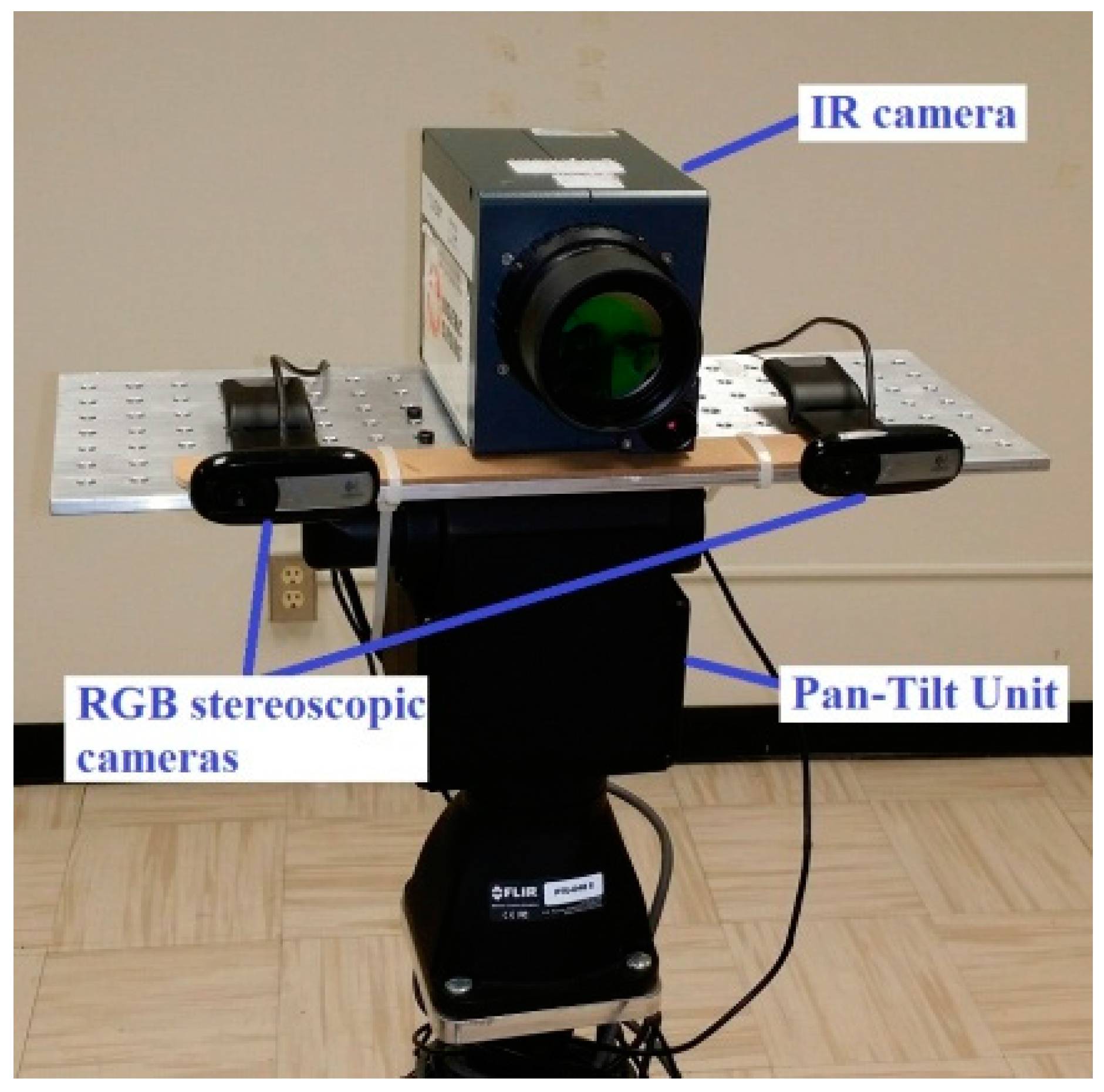
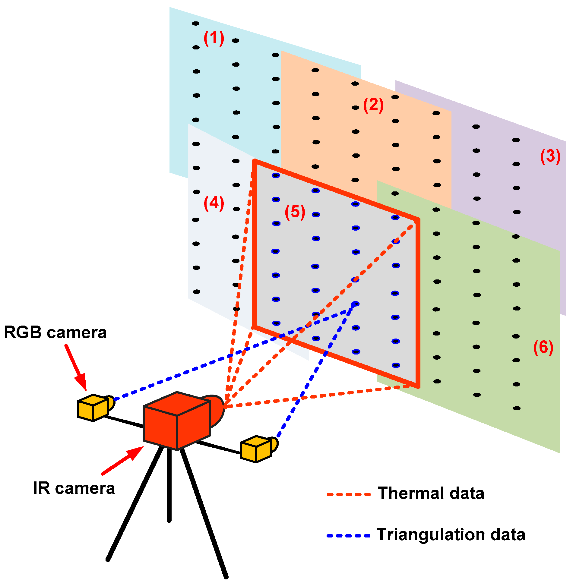
21]. They showed that the temperature history, recorded by an infrared camera, of a single sensor can be used to estimate air temperature, air speed, and the mean radiant temperature after solving an inverse heat transfer problem. A measurement grid, built by arranging several sensors in the field of view of the camera, is used to visualize the spatial distribution of each of these indoor parameters by interpolating punctual measurements given by each sensor. The main objective of this paper is to extend the field of application of infrared thermography to the mapping of the indoor ambient conditions. The proposed instrumentation has four components: A measurement grid, an infrared camera, a pair of stereoscopic cameras and a moving system. Four key points are addressed in order to ensure its reliability: the robust detection of the sensors in the images, the determination of the 3D coordinates of each sensor of the measurement grid, the evaluation in terms of accuracy and robustness of experimental performance achieved by the sensor, and the mapping of the indoor ambient conditions.
The paper is organized as follows: in the next section, we recall the theoretical fundamentals of the sensor. In the third section, we present the experimental validation of the sensor. In the fourth section, the dynamic Hough transform is used as a robust detection tool. We also present the determination of the 3D coordinates of each sensor by triangulation. In the fifth section, some experiments are conducted in order to quantify and to visualize the indoor parameters distribution in 2D and in 3D. The last section is the conclusion of the paper.

2. Theoretical Fundamentals of the Sensor

2.1. The Measurement Grid

Due to the fact that air is transparent, an auxiliary device is associated to the infrared camera in order to quantify and visualize the spatial distribution of the indoor ambient parameters. This auxiliary device, the measurement grid, is presented in Figure 1. It is composed of a set of spherical sensors (a), each having a diameter D S , arranged vertically and horizontally. A metal wire (b) of diameter D w D S passes through the sensors and is used to attach each row of sensors on the frame (c) and to heat the sensors by the Joule effect. A spring (d) maintains the wire straight, horizontally. The electric current needed for the Joule effect is provided by a voltage generator (e). Some mini-fans (f) allow the determination of the mean radiant temperature by modifying the heat exchange by convection between sensors and air.

2.2. Thermal Model of the Sensor

As Figure 2 shows, the sensor and the surroundings exchange heat by convection and by radiation at the rate Q ˙ c o n v and Q ˙ r a d , respectively. Between the wire and the sensor, there is heat exchange by conduction at the rate Q ˙ c o n d _ w . The rate of heat stored by the sensor is Q ˙ s t . For a thermally thin sensor, that is, for which the Biot number is less than 0.1, according to Incropera et al. [22], there is no internal temperature gradient; Q ˙ c o n d = 0 . Equation (1) gives then the thermal balance of the sensor. Q ˙ c o n d _ w is given by Equation (2) where Q J represents the heat produced by the Joule effect.
Q ˙ s t = Q ˙ c o n v + Q ˙ r a d + Q ˙ c o n d + Q ˙ c o n d _ w
Q ˙ c o n d _ w = { Q J   0   during the heating of the sensor during the cooling of the sensor
Considering the general case where the spherical metallic sensor, having a thickness e m , is covered by a high emissive paint of thickness e p , ideally e p e m , Equation (1) can be rewritten as below:
{ [ ( ρ c V ) p + ( ρ c V ) m ] d T d t = h A ( T T a i r ) σ ε A ( T 4 T r a d 4 ) + Q ˙ c o n d _ w T ( t = 0 ) = T 0
where subscripts p and m represent, respectively, the emissive component and the metallic component of the sensor. T 0 is the initial temperature and T is the temperature at time t . ρ is the density, c is the specific heat, V is the volume, A is the surface, ε is the emissivity, and h is the Convective Heat Transfer Coefficient (CHTC). T a i r is the air temperature around the sensor, T r a d is the Mean Radiant Temperature (MRT), and σ is the Stefan-Boltzmann constant. When a steady-state is achieved, the sensor has the temperature T e q and Equation (3) gives:
T r a d 4 = T e q 4 + h σ ε ( T e q T a i r ) Q ˙ c o n d _ w σ ε A
The insertion of Equation (4) into Equation (3) yields the following:
{ [ ( ρ c V ) p + ( ρ c V ) m ] d T d t = h A ( T T e q ) σ ε A ( T 4 T e q 4 ) T ( t = 0 ) = T 0

2.3. Estimation of the Ambient Parameters

Three of the four ambient parameters appear explicitly in Equations (4) and (5). They are air temperature T a i r , air speed v a i r through the CHTC h , and the mean radiant temperature T r a d . An inverse heat transfer problem has been solved in order to estimate these three parameters. After that, a transient regime is created on the sensor, its temperature history is recorded by the IR camera. If T = χ ( t , Θ , T 0 ) is the theoretical temperature history obtained after solving Equation (5) and T ˜ = χ ˜ ( t ) is the experimental temperature history given by the IR camera, the parameter estimation problem is the determination of the parameter vector Θ = [ h , T e q ] t r (superscript t r is the transpose operator) which minimizes the error function ξ given by:
ξ   =   m   =   1 m   =   M [ T m T ˜ m ] 2 = m   =   1 m   =   M [ χ ( t m , Θ , T 0 ) χ ˜ ( t m ) ] 2
A theoretical analysis of the presented model has been conducted by Djupkep et al. [21]. The influences of several parameters (the noise level of the experimental data, the initial temperature of the sensor, the thermo-physical properties of the sensor, the temporal length of the experimental data) on the accuracy of the model have been investigated. They found that one can expect the following uncertainties when the signal-to-noise ratio is greater than 53 d B and h 2 / h 1 > 3 :
Air temperature: Δ T a i r 0.5   ° C for 10   ° C T a i r 40   ° C and | T a i r T r a d | 20   ° C .
Mean radiant temperature: 0.5   ° C   Δ T r a d   1.5   ° C for 10   ° C T r a d 40   ° C and | T a i r T r a d |   20   ° C .
Air speed: 0.07   m / s   Δ v a i r 0.2   m / s for 0   m / s   v a i r 2   m / s .

3. Experimental Performance of the Sensor

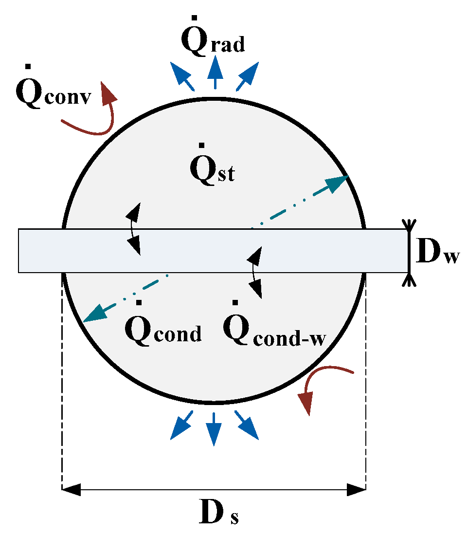
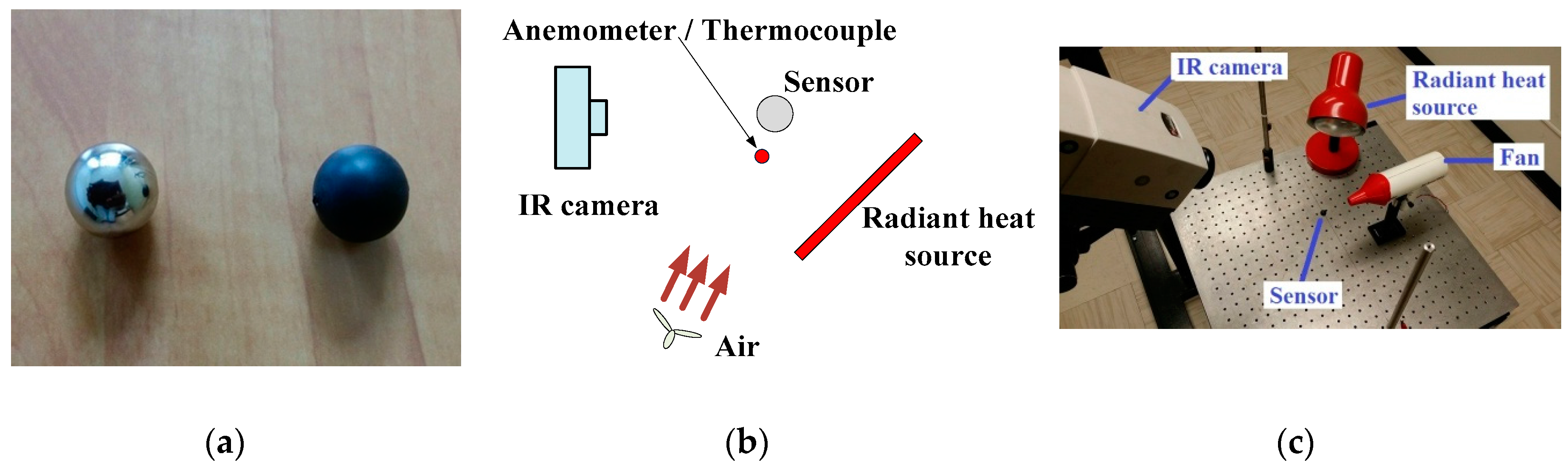
In order to accurately measure the sensor’s temperature using the infrared camera, the sensor, a hollow aluminum sphere, is covered with a high-emissivity acrylic paint (Figure 3a). The diameter of the sensor is 12   mm , the metallic part has a thickness of 1   mm , and the acrylic part has a maximum thickness of 0.2   mm and an emissivity of 0.96.
The experimental performances of the sensor are evaluated in terms of its reliability and the accuracy achieved on each of the three parameters measured. Our results are compared to the ISO 7726 standard [23]. The prescriptions of this standard are summarized in Table 1. The experimental setup (Figure 3b,c) consists of a fan that can provide air at various speeds and temperatures, a radiant heat source that can modify the amount of heat exchanged by radiation and the IR camera, which records the temperature history of the sensor.

3.1. Validation of the Thermal Model of the Sensor

The objective here is to verify that for all imposed conditions (air temperature, air speed, and MRT), the model (5) fits very well with the experimental data and that the estimated values are very close to the true imposed values. The sensor is heated by the Joule effect such that its temperature increased for at least 6   ° C . Then, the voltage generator is switched off and the sensor enters a transient regime during which its temperature is recorded by the IR camera during 5 min at a rate of five recordings per second. Figure 4a shows a typical experimental curve as well as the curve corresponding to the estimated parameters. As confirmed by Figure 4b, the difference between the estimated curve and the experimental curve is such that | T e x p ( t ) T e s t ( t ) | 0.2   ° C . When one of the three parameters (air temperature, air speed, and MRT) has a fixed value and the others change, we arrive to the same conclusion: The model (5) describes very well the thermal behavior of the sensor.

3.2. Validation of the Measurement of Air Speed
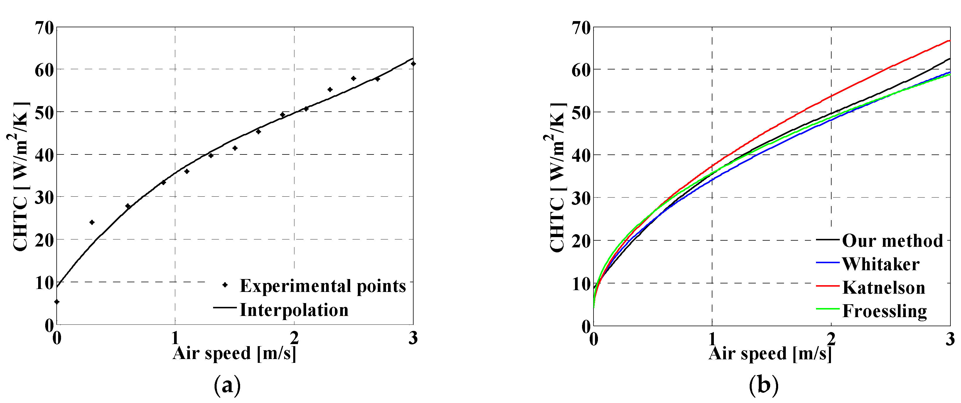
The CHTC h is estimated from the temperature history of the sensor. Air speed is then deduced. The correlation between the CHTC and the air speed has been sufficiently documented (Froessling [24], Katsnel'son and Timofeyeva [25], Whitaker [26]). Using our method, we determined a correlation between the CHTC and the air speed. Figure 3b,c shows the experimental setup used. A fan provides air flow at various speeds. The sensor is placed at 3   cm from the air exit. The value of the air speed is given by a hot wire anemometer having an uncertainty of 0.2   m / s and the air temperature is given by a thermocouple having an uncertainty of 0.5   ° C . The anemometer and the thermocouple have been chosen on the basis of the level of accuracy needed and their costs. For this work our goal was to meet the accuracy requirement of the standard ISO 7726. We achieved that with a low cost hot wire anemometer. During the calibration process, in order to reduce the measurement error resulting from the misalignment of the anemometer (thermocouple) and the air flow provided by the fan, several preliminary tests have been performed. The best position of the anemometer (thermocouple) was when the standard deviation of the measurements given by the anemometer (thermocouple) was less than its uncertainty.
Once the air speed is settled, the sensor is heated such that its temperature increased for at least 6   ° C . After that, the IR camera records the sensor temperature history while it cools. The following values of air speed have been imposed: ( 0 ; 0.3 ; 0.6 ; 0.9 ; 1.1 ; 1.3 ; 1.5 ; 1.7 ; 1.9 ; 2.1 ; 2.3 ; 2.5 ; 2.7 ; 3 )   ± 0.2   m / s . The air temperature has been maintained at ( 24 ± 0.5 )   ° C .
Figure 5a shows the curve, given by the proposed method, of the CHTC versus the air speed. As presented in Figure 5b, the resulting correlation is in accordance with existing correlations. The maximum error obtained on the air speed is 0.3   m / s . This maximum uncertainty is obtained for air speed equal to 3   m / s . For the same air speed, the standard ISO 7726 prescribes a desirable uncertainty of 0.2   m / s . This is of the same order of magnitude as that of the anemometer and is in accordance with the expected theoretical error for a signal to noise ratio SNR 50 dB [21]. The following relations are then written:
h = 1.81 v a i r 3 11.64 v a i r 2 + 36.56 v a i r + 8.77
v a i r = ( 0.69 h 2 + 7.30 h 111.40 ) × 10 3

3.3. Validation of the Measurement of Air Temperature and Mean Radiant Temperature

In order to modify the convective effect with respect to the radiative effect on the sensor, the air speed is modified such that two equilibria are created on the sensor. For each equilibrium, the parameters ( h 1 ,   T e q 1 ) and ( h 2 ,   T e q 2 ) are estimated. Using Equation (4), the air temperature and the mean radiant temperature are then determined respectively by Equation (9) and Equation (10):
T a i r = σ ε ( T e q 1 4 T e q 2 4 ) + h 1 T e q 1 h 2 T e q 2 ( h 1 h 2 )
T r a d = [ σ ε ( h 1 T e q 2 4 h 2 T e q 1 4 ) + h 1 h 2 ( T e q 2 T e q 1 ) σ ε ( h 1 h 2 ) Q ˙ c o n d _ w σ ε A ] 1 / 4
Using the experimental setup of Figure 3b,c, the temperature and the speed of the air supplied by the fan are kept to known values. The amount of heat exchanged by radiation between the sensor and its surrounding depends on the power of the lamp. For each trial, the MRT is kept constant by adjusting the power of the lamp to a constant value. The true value of the triplet ( v a i r ,   T a i r ,   T e q ) 
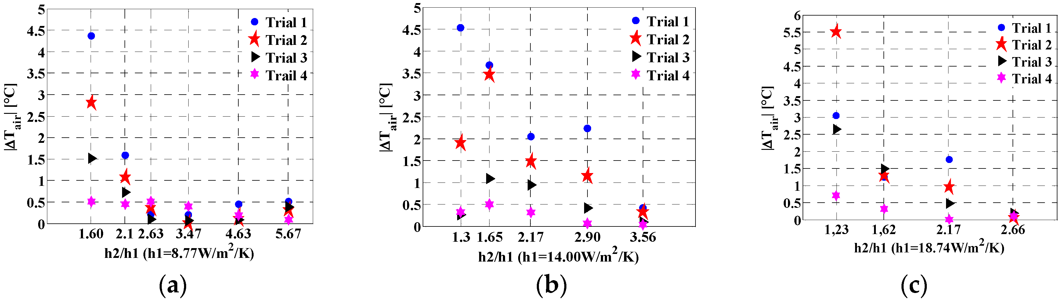
is known and serves as a reference for comparison. For each trial, seven air speeds are considered. The objective is to determine the ratio h 2 / h 1 for which the best accuracy on the measured parameters is achieved. For each of seven imposed air speeds, the temperature history of the sensor is used to estimate ( h ,   T e q ) . We then compose the couple { ( h ,   T e q ) i , ( h ,   T e q ) j } ; i j ; i , j = 1 , 2 , , 7 and compute the air temperature and the MRT using Equations (9) and (10), respectively. Table 2, with P 1 > P 2 > P 3 > P 4 , summarizes the experimental data considered.
Figure 6 gives the measurement error on the air temperature. It appears that, as the ratio h 2 / h 1 increases, the measurement error decreases. Furthermore, the value of h 1 also influences the accuracy of the measurement in that the accuracy is better for a small value of h 1 . In all cases, for h 2 / h 1 > 3 , the maximum measurement error is less than 0.6   ° C . There is a good agreement with the accuracy requirement of ISO 7726 [23].
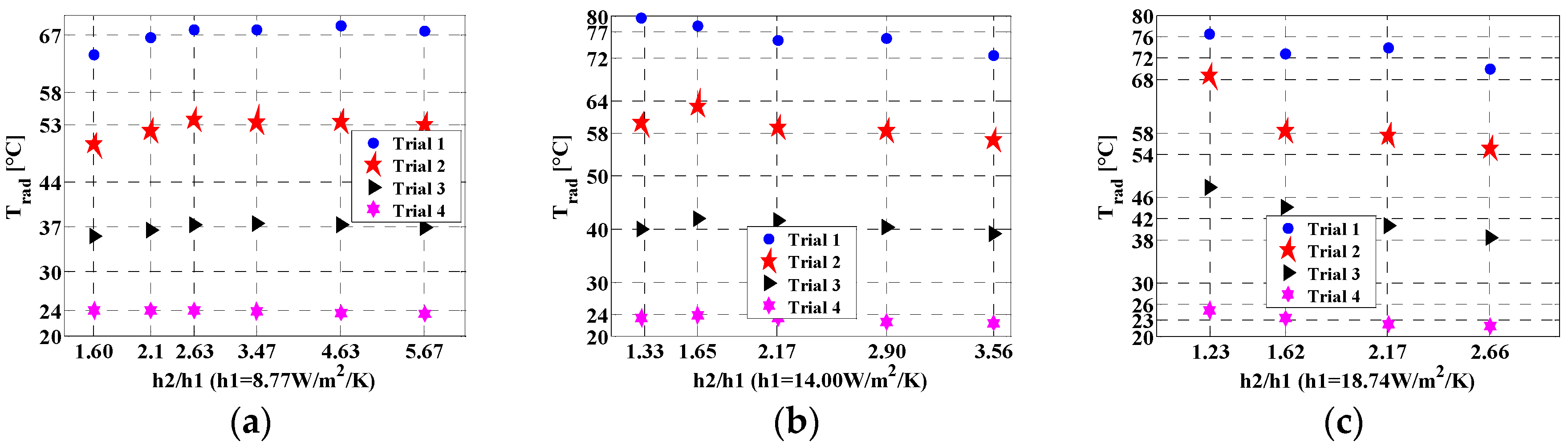
During the experiment, the true value of the MRT was not available. In order to validate our result, we made an assumption. As theoretical investigations suggest [21], there is a minimum value of the ratio h 2 / h 1 which guarantees a reliable measurement. For any ratio greater than that minimum value, the values found for the MRT must be the same. Consider Figure 7 showing the estimated MRT versus the ratio h 2 / h 1 for each trial. It is clear that the greater the ratio h 2 / h 1 , the better the accuracy as presented in Table 3. The value of h 1 has also a major influence. When h 1 is high (Figure 7b,c), the MRT values found, which were expected to be equal, vary significantly. The standard deviation is equal to 1.72   ° C for the first trial (Table 3). However, Figure 7a shows that for h 2 / h 1 > 2.63 , the MRT values found are close and show a standard deviation less than 1   ° C during each trial (Table 3). Thus, the method gives accurate results when h 2 / h 1 > 2.63 and h 1 is as small as possible. Of course, the best value of h 1 is the value corresponding to a null air speed.

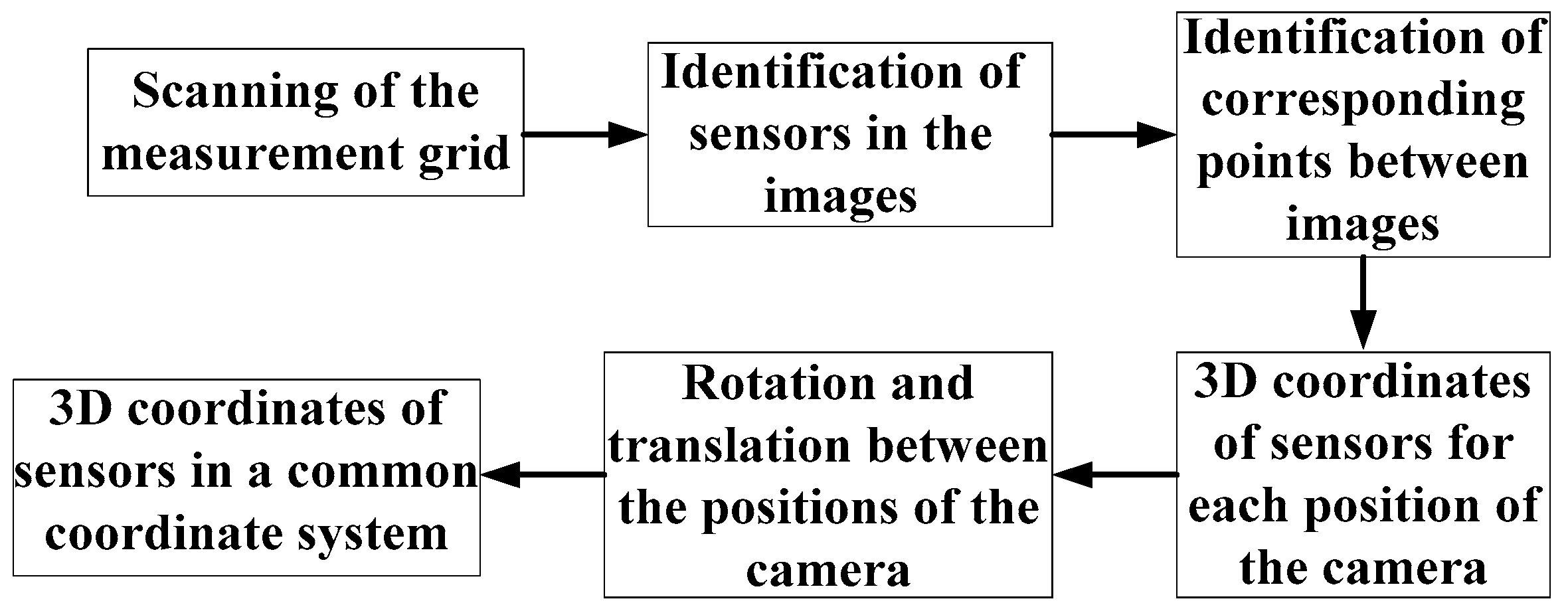
4. 3D Reconstruction of the Measurement Grid

The complete reconstruction of the measurement grid is achieved when the 3D coordinates of all of the sensors are known in a common coordinate system. These 3D coordinates are found by triangulation by stereovision; that is, by using a pair of cameras. The steps to follow in order to finalize the 3D reconstruction of the measurement grid are given in Figure 8.

4.1. Scanning of the Measurement Grid

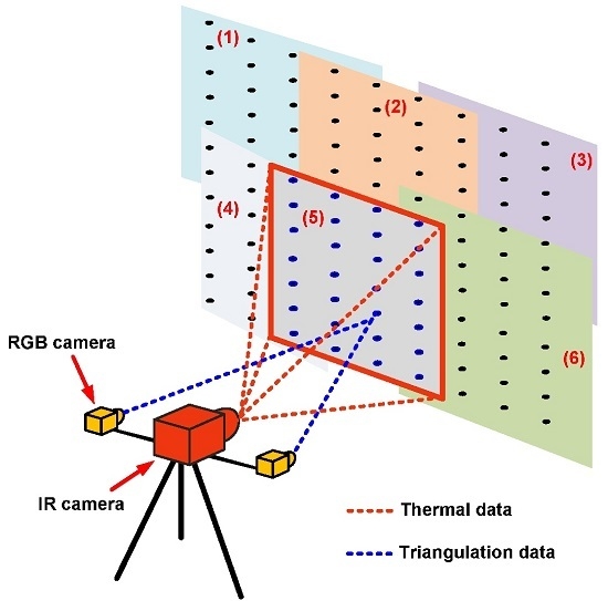
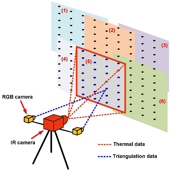
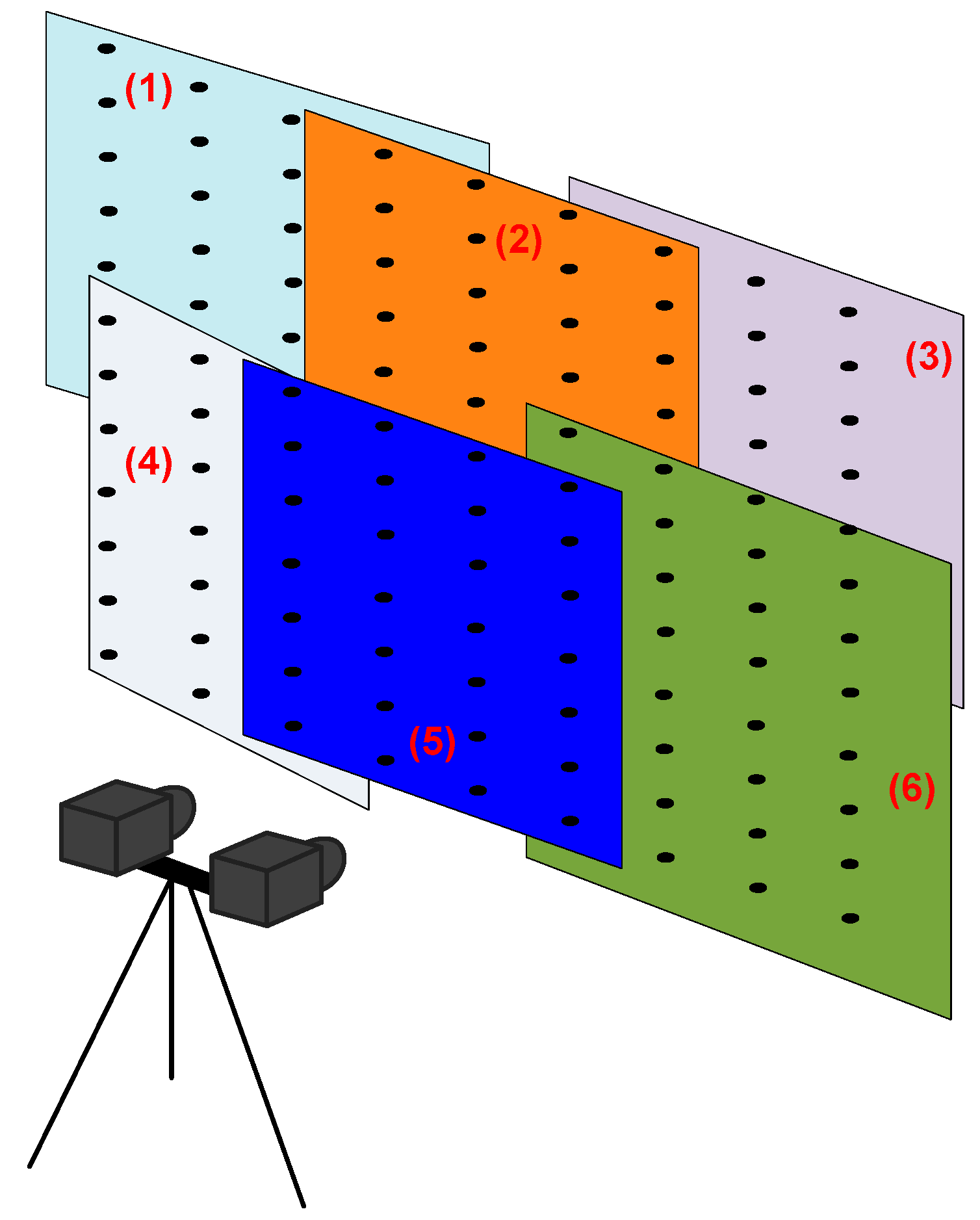
The field of view of the cameras is a limiting factor. Depending on the size of the measurement grid, cameras may not be able to simultaneously capture all of the sensors of the measurement grid. In such a case, the cameras are displaced from one position to the other in order to scan the entire measurement grid. Figure 9 shows an example of successive parts of the measurement grid during the scanning. Thanks to a pan-tilt unit, the motion of the cameras is possible. To complete the next steps, images recorded at two successive positions of the camera must overlap.

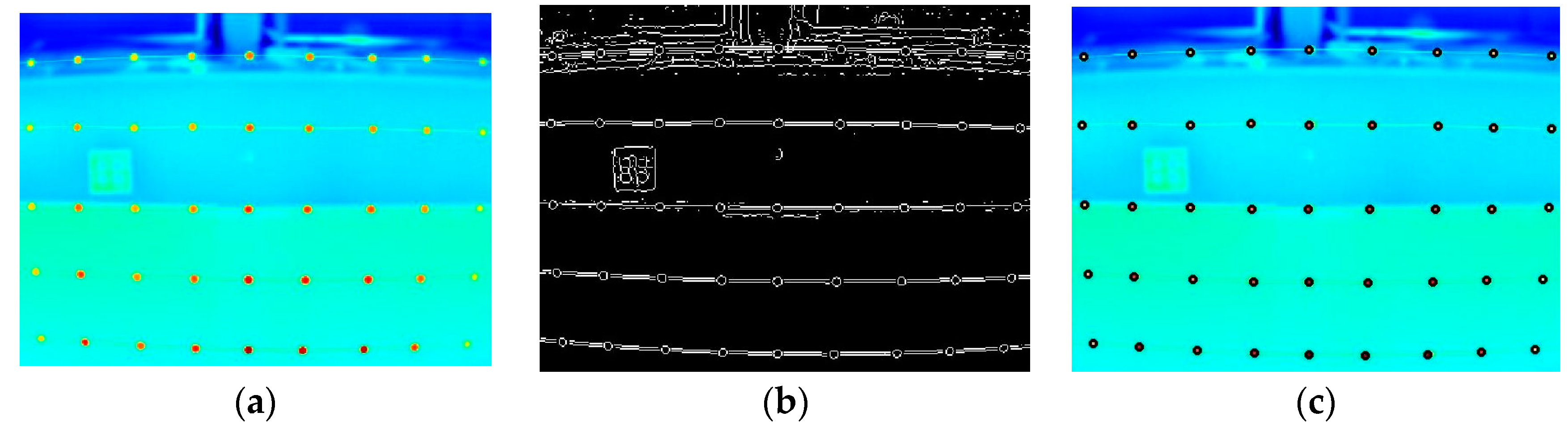
4.2. Detection of Sensors in the Images

The detection of the sensors of the measurement grid in the images aims to extract their temperature history and to determine their 3D coordinates. We use the Hough transform (Ioannoua et al. [27]) for the detection of our spherical sensors. The Hough transform is an algorithm which is easy to implement and has a high noise tolerance. It represents, in its parameter space, the geometrical shape to detect. To define a circle in a 2D Cartesian coordinate system, three parameters must be known: The coordinates ( c x ,   c y ) of the center and the radius r . Thus, in the parameter space, a circle is represented by the point ( c x ,   c y ,   r ) . The first step of the Hough transform is the detection of edge points in the image. Each edge point belongs hypothetically to the boundary of the searched circle. So, each of the detected edge points is represented in the parameter space. An accumulator is used such that each of its pixel coordinates represents a circle and the pixel value is equal to the number of edge points belonging to the searched circle. In the accumulator, the coordinates of local maxima are the representation of a real circle. Figure 10 shows the result of the sensors detection in an IR image by Hough transform.

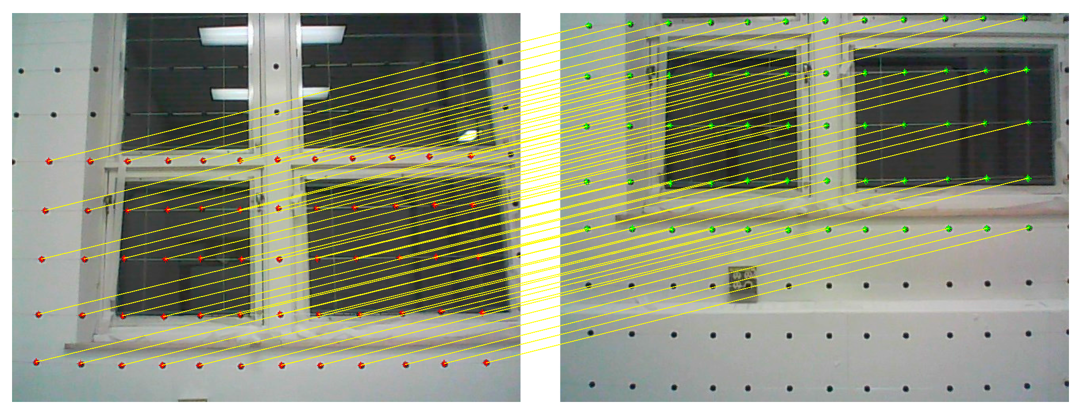
4.3. Corresponding Points between Images

A point m i in the image I 1 and a point m j of the image I 2 are called corresponding points if they represent the same real point [28]. In order to identify corresponding points between N 1 points in the image I 1 and N 2 points in the image I 2 , we can emphasize on the fact that two corresponding points must have a similar neighborhood. The level of similarity is given by the normalized cross correlation coefficient. The normalized cross correlation between the point m i and the point m j is:
N C C ( i , j ) = [ I 1 ( m i ) I ¯ 1 ] [ I 2 ( m j ) I ¯ 2 ] ( m i ) [ I 1 ( m i ) I ¯ 1 ] 2 ( m j ) [ I 2 ( m j ) I ¯ 2 ] 2
The neighborhood ( m ) , of the pixel m , includes all of the pixels belonging to a window of a given size centered on m . I ¯ is the mean value of these pixels. The corresponding point of m i is the point m j * such that N C C ( i , j * ) = max j = 1 , 2 , , N 2 [ N C C ( i , j ) ] .
Figure 11 presents an example of corresponding points between two RGB images corresponding to two positions of the camera.

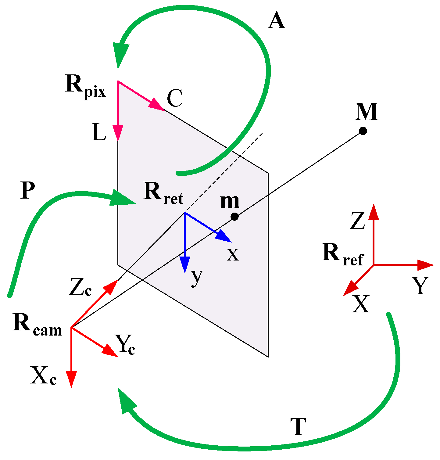
4.4. Geometric Calibration of A Camera

The objective of the geometric calibration of a camera is the identification and the determination of parameters of the mathematical model which exist between the 3D coordinates of a real point and its 2D coordinates in the image. The pinhole model (Hartley and Zisserman [28]) is the most popular model used to describe a camera. As illustrated in Figure 12, the camera projects the real point M ( X , Y , Z ) into the image point m ( C , L ) . This is possible after three transformations of the coordinate systems r e f ,   c a m ,   r e t ,   r e t d and p i x which are, respectively, the reference 3D coordinate system, the 3D coordinate system linked to the camera, the 2D retinal coordinate (without and with distortion) system belonging to the image plane, and the 2D pixel coordinate system. We have:
ref   cam ,   [ X C , Y C , Z C ] t r = R [ X , Y , Z ] t r + t
where R is the rotation matrix and t is the translation vector.
c a m   r e t ,   ( x , y ) = ( f X C / Z C ,   f Y C / Z C )
where f is the focal length of the camera lens.
r e t   r e t d ,   [ x d ,   y d ] = [ x , y ] ( 1 + d 1 r + d 2 r 2 + d 3 r 3 ) + [ d 4 ( 3 x 2 + y 2 ) + 2 d 5 x y , 2 d 4 x y + d 5 ( x 2 + 3 y 2 ) ]
where r = ( x 2 + y 2 ) and d i are the distortion parameters.
r e t d p i x ,   [ C , L ] = [ k x x d + k x y d c o t φ + C x + C y c o t φ , ( k y y d + C y ) / s i n φ ]
( C x , C y ) are the coordinates of the point where the optical axis of the camera lens meets the image plane, φ is the angle between the x axis and the y axis, k x and k y are the number of pixels per unit length. f x = f k x and f y = f k y .
Defining the intrinsic vector P i n = [ f x , f y , c x , c y , φ ,   d 1 , d 2 , d 3 , d 4 , d 5 ] and the extrinsic vector P e x = [ R 11 , R 12 , R 13 , R 21 ,   R 22 , R 23 , R 31 , R 32 , R 33 , t 1 , t 2 , t 3 ] , we write m = F ( P i n , P e x , M ) . The calibration consists then in determining the vectors P i n and P e x from a given set of corresponding points M m . 
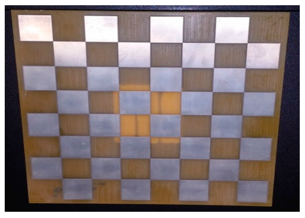
These points are found using a calibration target (Figure 13). The camera records N different images of the calibration target. The 3D coordinates of N p key points of the target (the corners of the squares in Figure 13) are known in a chosen 3D coordinate system and their 2D coordinates are known in the pixel coordinate system. Vectors P i n and P e x are determined such that the sum i = 1 i = N j = 1 j = N p m i j F ( P i n , P e x i , M j ) 2 has a minimum value (Heikkilä and Silven [29], Zhang [30]).

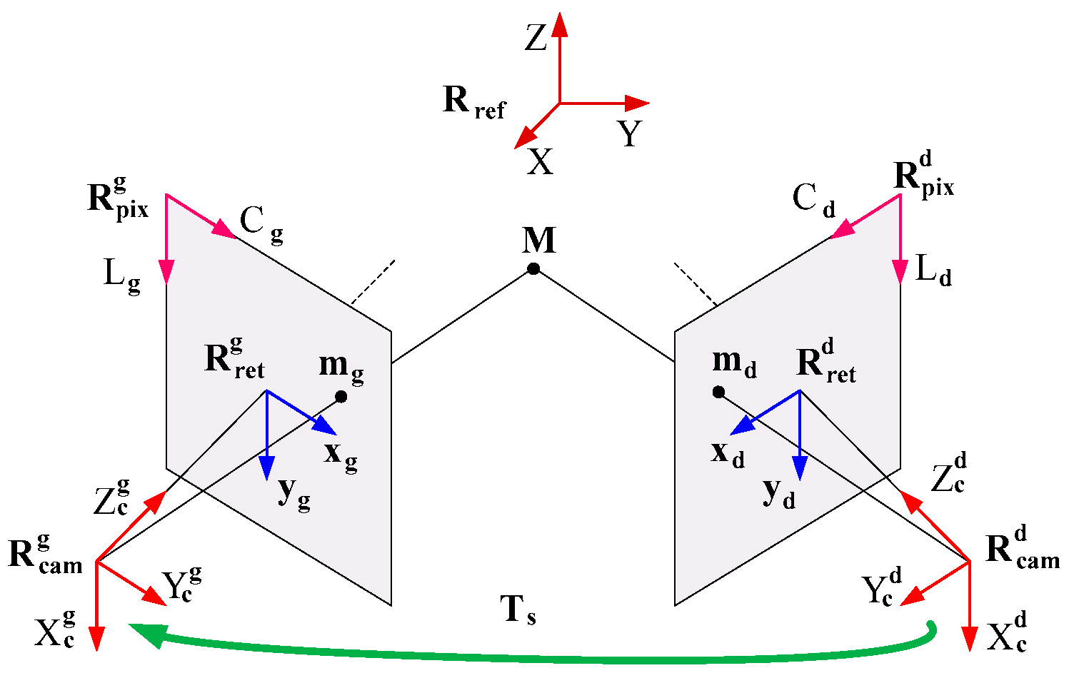
4.5. Triangulation by Stereoscopic Vision

Triangulation by stereoscopic vision is the determination of the 3D coordinates of a point using at least two cameras [31]. Considering a pair of stereoscopic cameras, Figure 14 presents the synoptic of the triangulation. The point M must be located simultaneously in the field of view of both cameras. If the point M is projected onto the point m l in the left image and onto the point m r in the right image, we can write m l = F ( ( P i n ) l , ( P e x ) l , M ) and m r = F ( ( P i n ) r , ( P e x ) r , M ) . If the intrinsic vectors, the extrinsic vectors, the points m l and m r are known, the two preceding equations can be solved in order to determine the 3D coordinates of the point M .
Instead of determining the 3D coordinates of M in an arbitrary 3D coordinate system, the coordinate system of one of the cameras can be used. In this case the rotation matrix R S and the translation vector t S between the coordinate systems of both cameras are determined by a calibration of the stereoscopic cameras. The calibration data are a set of N pairs of images of a calibration target having N p points. Each pair of images corresponds to a given spatial orientation of the calibration target. For the pair i ( i = 1 , 2 , , N ) , R S and t S can be determined using A S = ( A r ) i ( A l ) i 1 , with A S = [ R S t S 0 t r 1 ] , A r = [ R r t r 0 t r 1 ] and A l = [ R l t l 0 t r 1 ] .

4.6. Rotation and Translation between Two Positions of the Camera

Consider ( X 1 i , Y 1 i , Z 1 i ) and ( X 2 i , Y 2 i , Z 2 i ) , i = 1 , 2 , 3 , 4 , the coordinates of four points in the coordinate systems ( c a m ) P 1 and ( c a m ) P 2 of the camera, respectively, at the first and the second position. The rotation R 2 , 1 and the translation t 2 , 1 between coordinate systems ( c a m ) P 1 and ( c a m ) P 2 are such that ( X 1 i , Y 1 i , Z 1 i ) t r = t 2 , 1 + R 2 , 1 ( X 2 i , Y 2 i , Z 2 i ) t r . R 2 , 1 and t 2 , 1 are obtained by solving Equations (12).
M = [ 1 , X 2 1 , Y 2 1 , Z 2 1 1 , X 2 2 , Y 2 2 , Z 2 2 1 , X 2 3 , Y 2 3 , Z 2 3 1 , X 2 4 , Y 2 4 , Z 2 4 ] , { M [ t 1 , R 11 , R 12 , R 13 ] t r = [ X 1 1 , X 1 2 , X 1 3 , X 1 4 ] t r M [ t 2 , R 21 , R 22 , R 23 ] t r = [ Y 1 1 , Y 1 2 , Y 1 3 , Y 1 4 ] t r M [ t 3 , R 31 , R 32 , R 33 ] t r = [ Z 1 1 , Z 1 2 , Z 1 3 , Z 1 4 ] t r
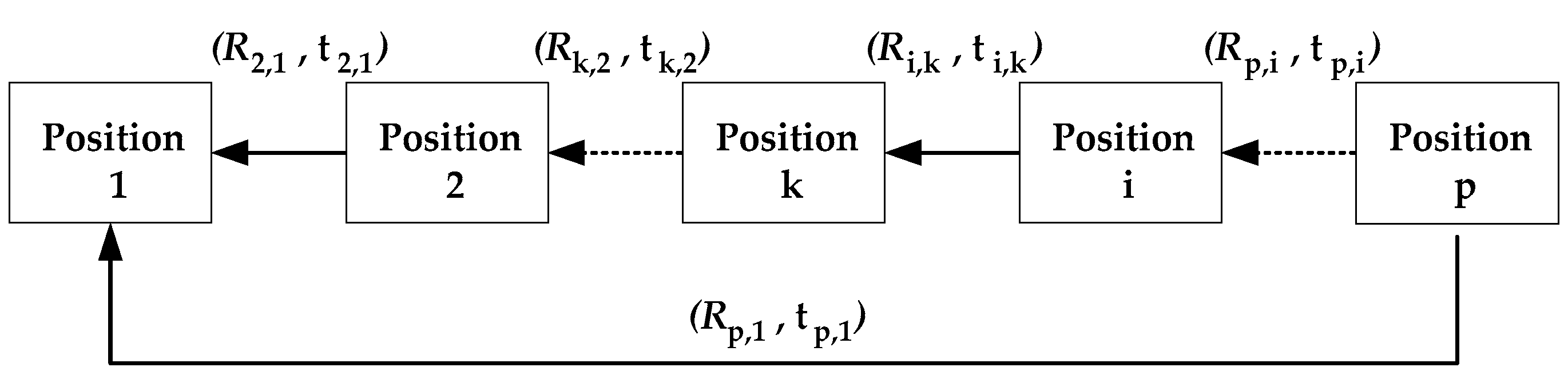
Suppose that for a complete scanning of the measurement grid, the camera passes through P different positions (Figure 10). The rotation R i , k and the translation t i , k (Figure 15) between coordinate systems ( c a m ) P i and ( c a m ) P k of the camera, respectively, at positions P i and P k are given by R i , k = j = k j = i 1 R j + 1 , j and t i , k = t k + 1 , k + [ l = 1 l = i k 1 ( j = k j = i l 1 R j + 1 , j ) t i l + 1 , i l ] .
Thus, if the coordinate system of the camera at position P 1 is taken as the common coordinate system, it is possible to determine the 3D coordinates of all of the sensors in that common system if we know all of the rotation matrices R i , 1 , the translation vectors t i , 1 and the 3D coordinates of the sensors in the coordinate system of the camera at position P i .

5. Mapping of the Indoor Parameters

5.1. Acquisition System

The acquisition system has three components and is presented in Figure 16. The IR camera is used to record thermal data from which the temperature of each sensor is obtained (Figure 17), the pair of stereoscopic RGB cameras is used to compute the 3D coordinates of the sensors by triangulation, and the pan-tilt unit serves to move the cameras during the scanning of the measurement grid. A web interface has been developed in order to ensure a synchronous working of these components and their control for short and long duration experiments. One can find the technical specifications in Béland et al. [32]. From the recorded temperature history, the indoor parameters are estimated for each sensor. By associating the value of the indoor parameter with the 3D coordinates of the point where this value has been measured, an interpolation is conducted and the mapping of the indoor parameter is obtained. Two experiments follow in order to illustrate the outcomes of the proposed instrumentation.

5.2. Example of 2D Mapping of Air Speed and Air Temperature above A Fan-Coil Unit

We present here the result of the quantification and the visualization of the air temperature and air speed in the median plane above a fan-coil. The fan-coil is installed under the windows of a room of size H × L × P = ( 2.5 × 2 × 3 )   m 3 as sketched in Figure 18a. The experimental setup is illustrated in Figure 18b. The measurement grid contains 48 sensors placed approximately at 10   cm intervals horizontally and 20   c m intervals vertically. This grid is placed 10   cm above the fan-coil and covers an area of ( 1 × 0.8 )   m 2 . All the sensors are in the field of view of the cameras, thus no camera motion is required. The mean external temperature is around 33   ° C and the fan-coil provides air at a constant temperature of 18   ° C . Three inlet air speeds ( v a i r 1 = 1.25   m / s , v a i r 2 = 1.95   m / s , and v a i r 3 = 2.80   m / s ), measured at the center of the fan-coil, are available.

5.2.1. 2D Mapping of the Air Speed

Figure 19 presents the 2D mapping of air speed for the three inlet air speeds of the fan-coil. Qualitatively, when the inlet air speed increases, the spatial distribution of the air speed has higher values. From these measurements, some characteristics can be retrieved. The horizontal profiles for heights 10   cm , 50   cm , and 90   cm above the fan coil are given by Figure 20. The profile at small heights (Figure 20a) is similar to the profile at the exit of the fan-coil. The air speed in this case is constant between 25   cm and 15   cm around the axis of the fan-coil. When the height increases, the profile becomes convex in shape with a maximum value around the main axis (Figure 20b). For higher heights (Figure 20c), the profile tends to become horizontal; a maximum penetration height exists. In order to determine this penetration height, we analyze the vertical profile (Figure 21) at the center axis of the fan-coil. The penetration height corresponds to the height at which air features are not influenced by the fan-coil. Before the switching-on of the fan-coil, the air speed is null along the room. We assume then that any air speed greater than zero is a result of the switching-on of the fan-coil. Taking into account the uncertainty of 0.3   m / s provided by the proposed instrumentation, we set the decision threshold to 0.3   m / s . Thus, the penetration height is the height at which the air speed is equal to 0.3   m / s . From Figure 21, the penetration height is identified as being 50   cm for the first inlet air speed, 68   cm for the second inlet air speed, and 84   cm for the third inlet air speed.

5.2.2. Air Thermal Stratification

Before the fan-coil is switched on, a thermocouple, placed at the center of the room, indicates ( 29.3 ± 0.5 )   ° C . Using our instrumentation, the mapping of the air temperature above the fan coil turned off is presented in Figure 22a. It shows that, in the room, the air temperature is not constant; there is a permanent thermal stratification. The air is hotter closer to the ceiling and cooler closer to the floor (Webster et al. [33]). It is clear from this result that the room's occupants could be subjected to local thermal discomfort due to the temperature difference between their ankles and their heads (Yu et al. [34]; ASHRAE Standard 55 [4]). Furthermore, in this situation where the room is in thermal equilibrium with the outdoors, isothermal lines are parallel to the floor (Figure 22b). Figure 22c shows the plot of the vertical temperature profile at the main axis of the fan-coil. It allows a quantification of the dependence between the temperature and the height in the stratified room. We see that the air temperature increases by 1   ° C when the height increases by 40   cm .

5.2.3. 2D Mapping of the Air Temperature

Air with a temperature of 18   ° C is supplied at three inlet speeds, v a i r 1 = 1.25   m / s , v a i r 2 = 1.95   m / s , and v a i r 3 = 2.80   m / s by the fan-coil. The air temperature distribution above the fan-coil is the result of a non-isothermal air flow in a portion of space where, initially, the air speed is null and the air temperature is given by Figure 22a. Figure 23 gives the mapping of the air temperature for the three inlet air speeds. Obviously, the initial temperature pattern (Figure 22a) is modified by the cold air supplied by the fan-coil. Instead of being horizontal, the isotherm lines now have a convex shape. For the lower inlet air speed for example, the air becomes stagnant from a certain height which is the penetration height (Figure 23a). One can also discuss the level of thermal comfort achieved when such a fan-coil is used. The temperature difference between the bottom and the top of the inspected area depends on the inlet air speed. For the first inlet air speed (Figure 23a), instead of 2   ° C as, initially, this temperature difference is greater than 10   ° C .

5.3. Example of 3D Mapping of Air Speed and Air Temperature above a Fan-Coil Unit

In this section we show that our instrumentation can be used successfully for the mapping of the indoor ambient parameters when the analyzed area is much greater than the field of view of the cameras. In such a case, the measurement grid is sufficiently large and a scanning is needed in order to record the temperature of all of the sensors. We apply the procedure to the mapping of the air speed and air temperature around a fan-coil which supplies hot air from the floor. The experimental setup is shown in Figure 24a. When the measurement grid is moved to several positions around the fan-coil, the 3D mapping of the parameters can be achieved. Figure 24b shows the four positions considered here for the mapping. Distances between the measurement grid and the median plane of the fan-coil are respectively 0   cm , 5   cm , 20   cm , and 35   cm . The measurement grid, in this case, covers an area of ( 1.2 × 1.7 )   m 2 and contains 286 sensors placed approximately at 8   c m intervals horizontally and 10   c m intervals vertically.
The motion of the cameras is ensured by the pan-tilt unit. At each position, the IR camera records a set of IR images corresponding to a partial view of the measurement grid, and the RGB cameras record a pair of stereoscopic images. From the IR images, the temperature history of the sensors is extracted; from each pair of stereoscopic images, their 3D coordinates are determined by triangulation. As presented in section 4, the rotation and the translation between coordinate systems of the camera for two successive positions can be determined. The 3D coordinates of all of the sensors can then be found in a common coordinate system. Figure 25a shows, for the first position of the measurement grid, the result of its 3D reconstruction. The reconstruction is slightly noisy due to errors which are introduced by the calibration of the cameras and the triangulation. By filtering this raw result using a RANSAC, we obtain the 3D coordinates of all 286 sensors (Figure 25b). Finally, Figure 25c gives the 3D coordinates of all of the sensors for the four positions of the measurement grid.
The problem here takes the form of a non-isothermal air flow where the mean inlet air temperature is 40   ° C , the mean inlet air speed is 1.5 m / s , the initial air temperature in the room is 23   ° C and, initially, air speed has a null value in the room. Figure 26 gives the results of the 3D mapping of air speed and air temperature. Coordinates ( 0 , 0 , 0 ) correspond to the origin of the coordinate system of the left camera. Thus, the proposed instrumentation provides a good mean for the visualization of the distribution of indoor parameters. For the present case where the fan-coil has a dimension of ( 10 × 56 )   cm 2 , it appears that, a significant impact of the fan-coil is noticeable only in a region close to its median plane; that is, at distances 0   cm and 5   cm from the median plane. Far from the fan-coil, the air temperature, as well as the air speed, has a quasi-uniform distribution.

6. Conclusions

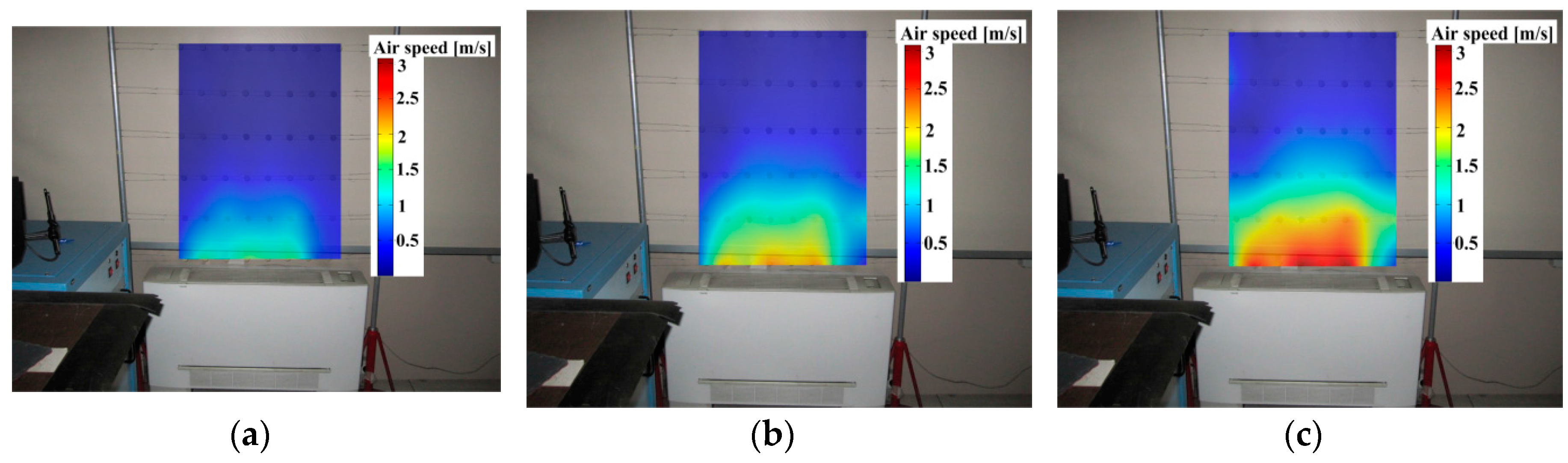
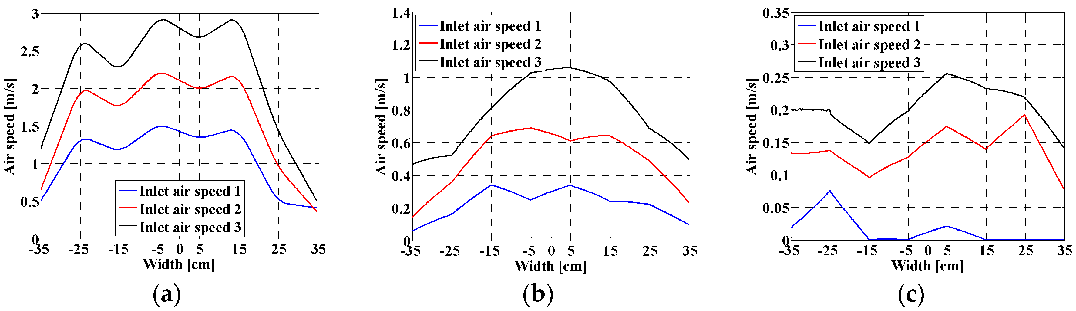
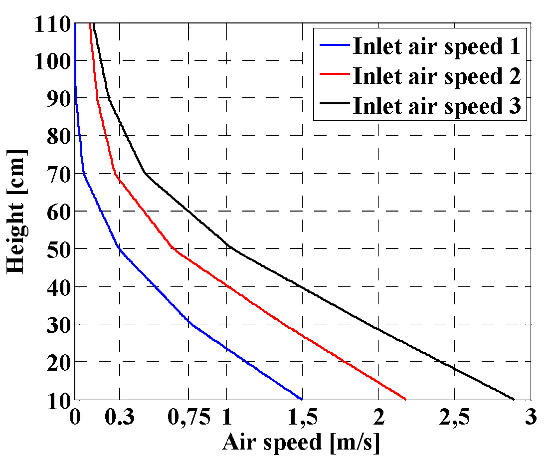
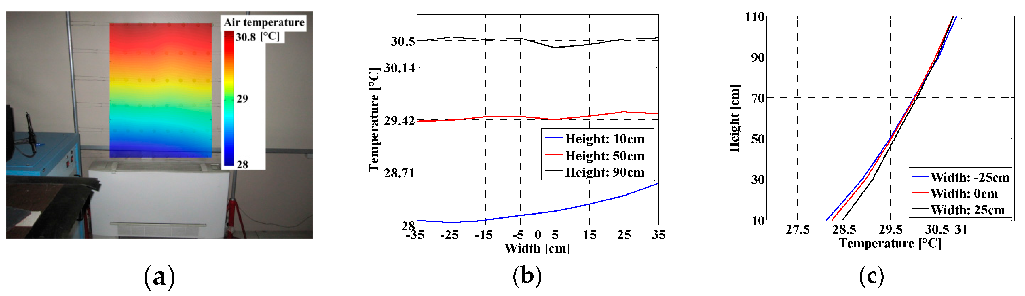
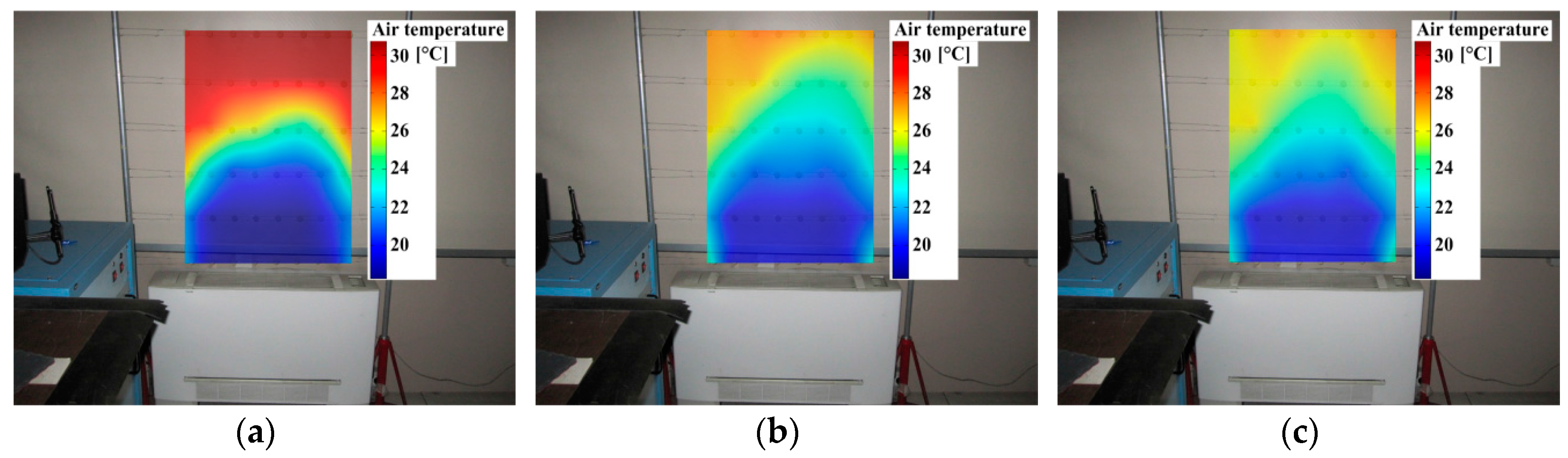
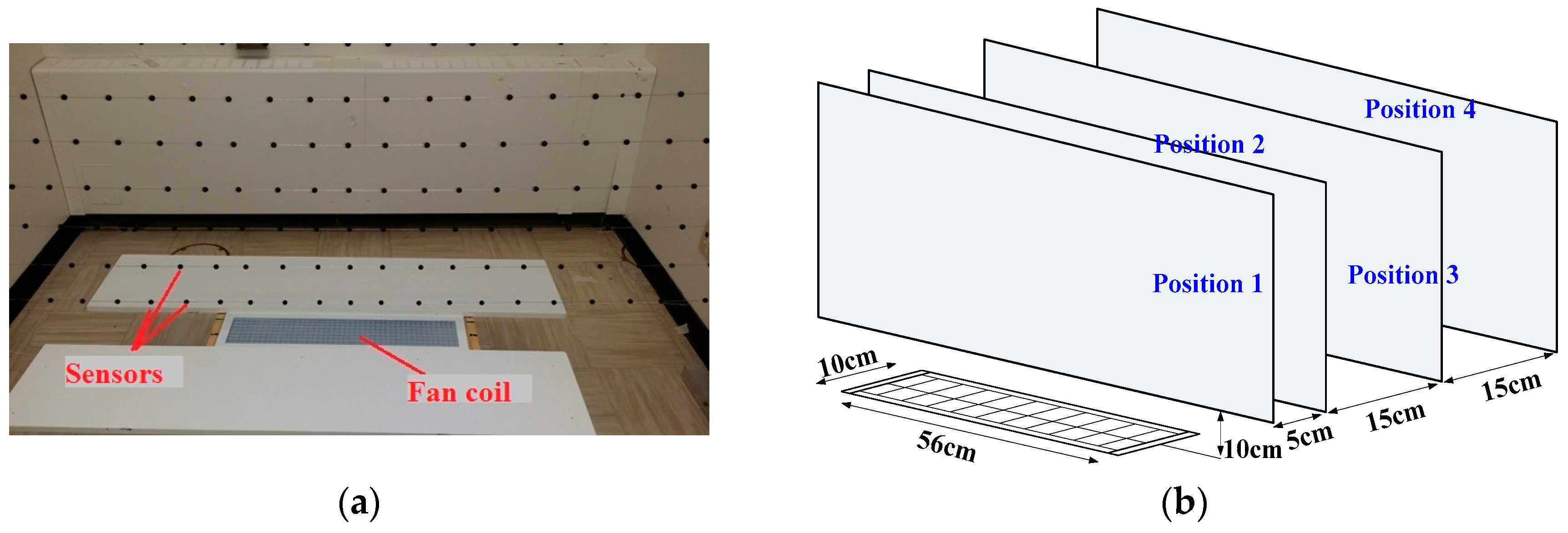
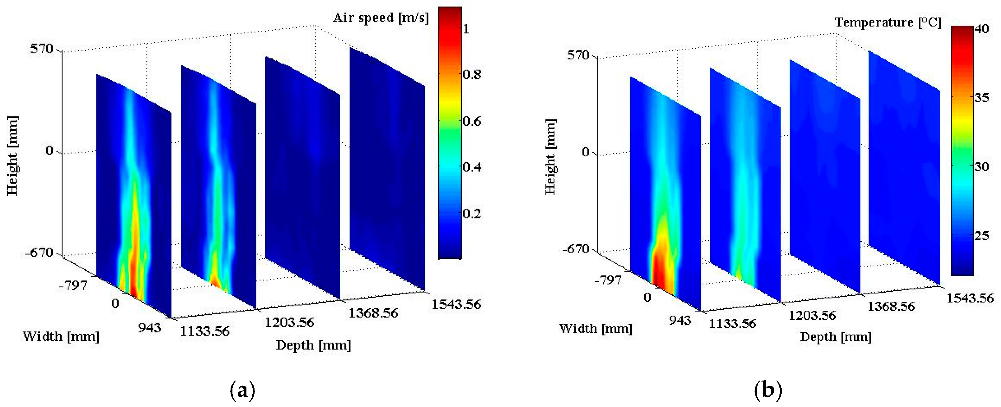
An instrumentation devoted to the mapping of the indoor conditions by infrared thermography has been presented. It is associated with a measurement grid built by arranging a set of sensors horizontally and vertically, an IR camera, a pair of stereoscopic RGB cameras and a pan-tilt unit. The sensor, which is used to determine all of the ambient parameters, has been validated experimentally. The results show that a maximum uncertainty of 0.3   m / s , 0.6   ° C and 1.7   ° C is achieved, respectively, on air speed, air temperature, and mean radiant temperature, respectively. Image processing tools have been presented. The objectives achieved are the robust detection of sensors in the images through Hough transform, the determination of the 3D coordinates of the sensors by triangulation, and the registration of all of the sensors in a common 3D coordinate system, specifically when the camera is moved in order to scan the entire measurement grid. The full procedure works very well and the mapping of the indoor parameters is possible. Two in situ experiments have been conducted. The first experiment involved the 2D mapping of air temperature and speed above a cooling fan-coil unit, and the second experiment involved the 3D mapping of air temperature and speed around a heating fan-coil unit. Results show that the instrumentation proposed is reliable and can be regarded as both a measurement technique and a visualization technique. All of the experiments presented in this paper have been conducted in office buildings without any occupants. At this time, no experiment has been conducted in the presence of occupants. As the method uses an infrared camera, there must be a free path between the camera and all of the sensors of the measurement grid. This is the main constraint of the proposed method. For the experiments where occupants are present, a difficulty could be to find the best way to place the measurement grid such that it is visible by the camera. Let us remind that, instead of using three different sensors, the proposed method uses a simple metallic spherical sensor for the contactless measurement of three different ambient parameters. From this point of view, the method has a low economic cost, particularly for the mapping of these parameters. A simple distribution of such sensors (measurement grid) in space can provide useful data for the mapping. The use of the dedicated instruments (anemometer, thermocouple, etc.) will result in a point-to-point process which is very time consuming and cumbersome. At this time one drawback of the method is its accuracy level. Although it meets the requirement of accuracy of the standard ISO 7726, some improvements is needed to also meet the desirable accuracy prescribed by the standard. Specifically, a more accurate and sensitive anemometer has to be considered for calibration. Furthermore, a camera with a high spatial resolution may improve the signal-to-noise ratio of the experimental data.

Acknowledgments

The authors want to thank the Chaire de recherche du Canada Multipolar Infrared Vision – Vision Infrarouge Multipolaire (MIVIM), Natural Sciences and Engineering Research Council of Canada (NSERC) and the Ministère des relations internationales, de la francophonie et du commerce extérieur du Québec, commission Québec-Italie for their financial support and Annette Schwerdtfeger for proofreading the manuscript.

Author Contributions

Xavier Maldague, Frank Billy Djupkep Dizeu and Abdelhakim Bendada conceived the study. Frank Billy Djupkep Dizeu prepared and wrote the manuscript. Xavier Maldague and Abdelhakim Bendada provided useful assistance in improving the quality of the manuscript.

Conflicts of Interest

The authors declare no conflict of interest.

References

  1. Olesen, B.W.; Parsons, K.C. Introduction to thermal comfort standards and to the proposed new version of EN ISO 7730. Energy Build. 2002, 34, 537–548. [Google Scholar] [CrossRef]
  2. D’Ambrosio Alfano, F.R.; Dell’Isola, M.; Palella, B.I.; Riccio, G.; Russi, A. On the measurement of the mean radiant temperature and its influence on the indoor thermal environment assessment. Build. Environ. 2013, 63, 79–88. [Google Scholar] [CrossRef]
  3. Dell’Isola, M.; Frattolillo, A.; Palella, B.I.; Riccio, G. Measurement uncertainties influence on the thermal environment assessment. Int. J. Thermophys. 2012, 33, 1616–1632. [Google Scholar] [CrossRef]
  4. ASHRAE Standard 55. Thermal Environmental Conditions for Human Occupancy; American Society of Heating, Refrigerating and Air Conditioning Engineers: Atlanta, GA, USA, 2013. [Google Scholar]
  5. ISO 7730. Ergonomics of the Thermal Environment-Analytical Determination and Interpretation of Thermal Comfort Using Calculation of the PMV and PPD Indices and Local Thermal Comfort Criteria; International Standardisation Organisation: Geneva, Switzerland, 2005. [Google Scholar]
  6. EN 15251. Indoor Environmental Input Parameters for Design and Assessment of Energy Performance of Buildings Addressing Indoor Air Quality, Thermal Environment, Lighting and Acoustics; European Committee for Standardization: Brussels, Belgium, 2007. [Google Scholar]
  7. Fraden, J. Handbook of Modern Sensors; Springer: New York, NY, USA, 2004. [Google Scholar]
  8. Parsons, K.C. Human Thermal Environments: The Effects of Hot, Moderate, and Cold Environments on Human Health, Comfort and Performance, 2nd ed.; Taylor and Francis: London, UK, 2003. [Google Scholar]
  9. Sun, Y.; Zhang, Y. An overview of room air motion measurement: Technology and application. HVAC&R Res. 2007, 13, 929–950. [Google Scholar]
  10. Sandberg, M. Whole-field measuring methods in ventilated rooms. HVAC&R Res. 2007, 13, 951–970. [Google Scholar]
  11. Dactu, S.; Ibos, L.; Candau, Y.; Mattei, S. Improvement of building wall surface temperature measurements by infrared thermography. Infrared Phys. Technol. 2005, 46, 451–467. [Google Scholar]
  12. Grinzato, E.; Vavilov, V.; Kauppinen, T. Quantitative infrared thermography in buildings. Energy Build. 1998, 29, 1–9. [Google Scholar] [CrossRef]
  13. Grinzato, E.; Cadelano, G.; Bison, P. Moisture map by IR thermography. J. Mod. Opt. 2010, 57, 1770–1778. [Google Scholar] [CrossRef]
  14. Balaras, C.A.; Argiriou, A.A. Infrared thermography for building diagnostics. Energy Build. 2002, 34, 171–183. [Google Scholar] [CrossRef]
  15. Choi, J.K.; Mik, K.; Sagawa, S.; Shiraki, K. Evaluation of mean skin temperature formulas by infrared thermography. Int. J. Biom. 1997, 41, 68–75. [Google Scholar] [CrossRef]
  16. Korukçu, Ö.; Kılıç, M. The usage of IR-thermography for the temperature measurements inside an automobile cabin. Int. Comm. Heat Mass Transf. 2009, 36, 872–877. [Google Scholar] [CrossRef]
  17. Shastri, D.; Papadakis, M.; Tsiamyrtzis, P.; Bass, B.; Pavlidis, I. Perinasal imaging of physiological stress and its affective potential. IEEE trans. Affect. Comput. 2012, 3, 366–378. [Google Scholar] [CrossRef]
  18. Fokaides, P.A.; Jurelionis, A.; Gagyte, L.; Kalogirou, S.A. Mock target IR thermography for indoor air temperature measurement. Appl. Energy 2016, 164, 676–685. [Google Scholar] [CrossRef]
  19. Cehlin, M.; Moshfegh, B.; Sandberg, M. Measurements of air temperatures close to a low velocity diffuser in displacement ventilation using infrared camera. Energy Build. 2002, 34, 687–698. [Google Scholar] [CrossRef]
  20. Pretto, A.; Menegatti, E.; Bison, P.; Grinzato, E. Automatic indoor environmental conditions monitoring by IR thermography. In Proceedings of 6th International Workshop for Advances in Signal Processing for NDE of Materials, London, ON, Canada, 25–27 August 2009.
  21. Djupkep, F.B.D.; Maldague, X.; Bendada, A.; Bison, P. Analysis of a new method of measurement and visualization of indoor conditions by infrared thermography. Rev. Sci. Instrum. 2013, 84, 084906. [Google Scholar] [CrossRef] [PubMed]
  22. Incropera, F.P.; Dewitt, D.P.; Bergman, T.L.; Lavine, A.S. Fundamentals of Heat and Mass Transfer, 6th ed.; John Wiley & Sons: New York, NY, USA, 2007. [Google Scholar]
  23. ISO 7726. Ergonomics of the Thermal Environment-Instruments for Measuring Physical Quantities; International Standardisation Organisation: Geneva, Switzerland, 2002. [Google Scholar]
  24. Froessling, N. Ueber die Verdunstung fallender Tropfen. Gerlands Beitr. Geophys. 1938, 52, 170–216. [Google Scholar]
  25. Katsnel’son, B.D.; Timofeyeva, F.A. Study of convective heat transfer between particles and flow under non-steady-state conditions. In Fundamentals of Heat Transfer; Kutateladze, S.S., Ed.; Edward Arnold: London, UK, 1963. [Google Scholar]
  26. Whitaker, S. Forced convection heat transfer correlations for flow in pipes, past flat plates, single cylinders, single spheres, and for flow in packed beds and tube bundles. AlChE J. 1972, 18, 361–371. [Google Scholar] [CrossRef]
  27. Ioannoua, D.; Hudab, W.; Laine, A.F. Circle recognition through a 2D Hough transform and radius histogramming. Imag. Vision Comput. 1999, 17, 15–26. [Google Scholar] [CrossRef]
  28. Hartley, R.I.; Zisserman, A. Multiple View Geometry in Computer Vision; Cambridge University Press: Cambridge, UK, 2004. [Google Scholar]
  29. Heikkilä, J.; Silven, O. A four-step camera calibration procedure with implicit image correction. In Proceedings of the 1997 IEEE Computer Vision and Pattern Recognition, San Juan, Puerto Rico, 17–19 June 1997.
  30. Zhang, Z. A flexible new technique for camera calibration. IEEE Trans. Anal. Mach. Intell. 2000, 22, 1330–1334. [Google Scholar] [CrossRef]
  31. Hartley, R.I.; Sturm, P. Triangulation. Comput. Vision. Imag. Underst. 1997, 68, 146–157. [Google Scholar] [CrossRef]
  32. Béland, M.-A.; Djupkep, F.B.D.; Bendada, A.; Maldague, X.; Ferrarini, G.; Bison, P.; Grinzato, E. Design of a remote infrared images and other data acquisition station for outdoor applications. Proc. SPIE 2013, 8705. [Google Scholar] [CrossRef]
  33. Webster, T.; Bauman, F.; Reese, J. Underfloor air distribution: Thermal stratification. ASHRAE J. 2002, 44, 28–36. [Google Scholar]
  34. Yu, W.J.; Cheong, W.D.; Sekhar, S.C.; Tham, K.; Kosonen, W. Local discomfort caused by draft perception in a space served by displacement ventilation system in the tropics. Indoor Built Environ. 2006, 15, 225–233. [Google Scholar] [CrossRef]
Figure 1. Measurement grid [21]. Reprinted with permission from Rev. Sci. Instrum., 84, 084906 (2013). Copyright 2013 American Institute of Physics.
Jimaging 02 00010 g001
Figure 2. Thermal model of the sensor [21]. Reprinted with permission from Rev. Sci. Instrum., 84, 084906 (2013). Copyright 2013 American Institute of Physics.
Jimaging 02 00010 g002
Figure 3. Performance of the sensor. (a) Sensor without (left) and with (right) the high-emissivity paint; (b) synoptic of the experimental setup; and (c) the experimental setup.
Jimaging 02 00010 g003
Figure 4. Typical curves; (a) experimental and estimated curves; and (b) difference between both curves.
Jimaging 02 00010 g004
Figure 5. CHTC versus air speed. (a) Experimental results; and (b) comparison with other correlations.
Jimaging 02 00010 g005
Figure 6. Measurement error on air temperature versus the ratio h 2 / h 1 . (a) h 1 = 8.77   W / m 2 / K ; (b) h 1 = 14.00   W / m 2 / K ; and (c) h 1 = 18.74   W / m 2 / K .
Jimaging 02 00010 g006
Figure 7. MRT measured versus the ratio h 2 / h 1 . (a) h 1 = 8.77   W / m 2 / K ; (b) h 1 = 14.00   W / m 2 / K ; and (c) h 1 = 18.74   W / m 2 / K .
Jimaging 02 00010 g007
Figure 8. Synoptic of the 3D reconstruction of the measurement grid.
Jimaging 02 00010 g008
Figure 9. Scanning of the measurement grid. (1) to (6): partial views of the measurement grid corresponding to the successive positions of the stereoscopic cameras.
Jimaging 02 00010 g009
Figure 10. Sensors detection in an IR image. (a) Original image; (b) edge points image; and (c) detected sensors.
Jimaging 02 00010 g010
Figure 11. Corresponding points between two RGB images.
Jimaging 02 00010 g011
Figure 12. 3D–2D projection.
Jimaging 02 00010 g012
Figure 13. Calibration target.
Jimaging 02 00010 g013
Figure 14. Triangulation by stereovision.
Jimaging 02 00010 g014
Figure 15. Rotation and translation between positions of the camera.
Jimaging 02 00010 g015
Figure 16. Acquisition system.
Jimaging 02 00010 g016
Figure 17. Data retrieved during the scanning. (1) to (6): partial views of the measurement grid corresponding to the successive positions of the cameras.
Jimaging 02 00010 g017
Figure 18. 2D mapping above a fan-coil. (a) Fan-coil position in the room; and (b) scheme of the experimental setup.
Jimaging 02 00010 g018
Figure 19. 2D mapping of the air speed above a fan-coil. (a) Inlet air speed v a i r 1 = 1.25   m / s ; (b) inlet air speed v a i r 2 = 1.95   m / s ; and (c) inlet air speed v a i r 3 = 2.80   m / s .
Jimaging 02 00010 g019
Figure 20. 2D mapping of the air speed above a fan-coil, horizontal profiles. (a) Height of 10   cm ; (b) height of 50   cm ; and (c) height of 90   cm .
Jimaging 02 00010 g020
Figure 21. 2D mapping of the air speed above a fan-coil, vertical profile at the center axis.
Jimaging 02 00010 g021
Figure 22. Air stratification. (a) Air temperature spatial distribution; (b) horizontal profiles; and (c) vertical profile at the center axis.
Jimaging 02 00010 g022
Figure 23. 2D mapping of the air temperature above a fan-coil. (a) Inlet air speed v a i r 1 = 1.25   m / s ; (b) inlet air speed v a i r 2 = 1.95   m / s ; and (c) inlet air speed v a i r 3 = 2.80   m / s .
Jimaging 02 00010 g023
Figure 24. 3D mapping above a fan-coil. (a) Experimental setup; and (b) successive positions of the measurement grid.
Jimaging 02 00010 g024
Figure 25. 3D coordinates of the sensors. (a) Raw data of the triangulation; (b) filtered data; and (c) the reconstructed measurement grid for the four positions.
Jimaging 02 00010 g025
Figure 26. 3D mapping. (a) Case of air speed; and (b) case of air temperature.
Jimaging 02 00010 g026
Table 1. Accuracy prescriptions of the standard ISO 7726 (response time as short as possible).
QuantityClass C (Comfort)Class S (Thermal Stress)
Measuring RangeAccuracyMeasuring RangeAccuracy
Air speed[0.05; 1] m/sRequired:
±(0.05 + 0.05vair) m/s a
Desirable:
±(0.02 + 0.07vair) m/s a
[0.2; 20] m/sRequired:
±(0.1 + 0.05vair) m/s a
Desirable:
±(0.05 + 0.05vair) m/s a
Air temperature[10; 40] °CRequired: ±0.5 °C b
Desirable: ±0.2 °C b
[−40; 120] °CRequired:
[−40; 0]°C: ±(0.5 + 0.01|Tair|) °C c
[0; 50] °C: ±0.5 °C c
[50; 120] °C:
±(0.5+0.04(Tair − 50)) °C c
Desirable: required/2 c
Mean radiant temperature[10; 40] °CRequired: ±2 °C
Desirable: ±0.2 °C
When the levels cannot be achieved, indicate the actual measuring precision.
[−40; 150] °CRequired:
[−40; 0] °C: ±(5 + 0.02|Tair|) °C
[0; 50] °C: ±5 °C
[50; 150] °C:
±(5+0.08(Trad − 50))°C
Desirable:
[−40; 0] °C: ±(0.5 + 0.01|Trad|)°C
[0; 50] °C: ±5 °C
[50; 150] °C:
±(0.5 + 0.04(Trad − 50)) °C
a: These levels shall be guaranteed whatever the direction of flow within a solid angle 3πsr; b: These levels shall be guaranteed at least for |Tair − Trad| ≤ 10 °C; c: these levels shall be guaranteed at least for |Tair − Trad| ≤ 20 °C.
Table 2. Experimental data.
TrialAir Temperature (°C)Lamp PowerAir Speed (m/s)
CHTC (W/m2/K)
Δ v a i r (m/s)
1234567
125.5 ± 0.5P10
8.77
0.15
14.00
0.30
18.74
0.45
23.03
0.75
30.41
1.30
40.60
2.00
49.81
0.2
2P2
3P3
4P4 = 0
Table 3. Mean value and standard deviation of the measured mean radiant temperature.
Trial h 2 / h 1 > 2.63
h 1 = 8.77   W / m 2 / K
h 2 / h 1 > 1.60
h 1 = 8.77   W / m 2 / K
h 2 / h 1 > 1.60
h 1 = 14.00   W / m 2 / K
Mean ValueStandard DeviationMean ValueStandard DeviationMean ValueStandard Deviation
167.91 °C0.75 °C67.00 °C1.67 °C74.55 °C1.72 °C
253.32 °C0.69 °C52.53 °C1.42 °C57.98 °C1.22 °C
337.29 °C0.42 °C36.88 °C0.73 °C40.38 °C1.26 °C
423.73 °C0.22 °C23.80 °C0.22 °C22.84 °C0.52 °C

