Dilemma Zone: Modeling Drivers’ Decision at Signalized Intersections against Aggressiveness and Other Factors Using UAV Technology

Abstract

Intersection safety and drivers’ behavior are strongly interrelated, especially when the latter are located in dilemma zone. This paper explores, among others, the main factors affecting driver behavior, such as distance to stop line, approaching speed and acceleration/deceleration, and two additional factors, namely, driver’s aggressiveness and driver’s relative position at the onset of the yellow signal. Field data were collected using unmanned aerial vehicle (UAV) technology. Two binary choice models were developed, the first relying on observed data and the latter enriched by the latent factor drivers’ aggressiveness and the vehicles’ relative position. Drivers were classified to aggressive and non-aggressive ones using a latent class model that combined approaching speed and acceleration/deceleration data. Drivers were further grouped according to their expected reaction/decision to stop or cross the intersection in relation to their relative position. Both models equally explain drivers’ decisions adequately, but the second one offers additional explanatory power attributed to aggressiveness. Being able to identify the level of aggressiveness among the drivers enables the calculation of the probability that drivers will cross the intersection even if caught in a dilemma zone or in a zone in which the obvious decision is to stop. Such findings can be valuable when designing a signalized intersection and the traffic time settings, as well as the posted speed limit.

1. Introduction

Given the variety of participants’ behaviors and interactions, road intersections are broadly believed to be the highest risk areas of road networks [1]. Worldwide accident statistics across the regions indicate that the majority of all traffic accidents occur at intersections, some of which are signalized. According to accident data available for the metropolitan area of Thessaloniki, Greece, for the time period 2013–2016, about 44% of all road accidents occurred at intersections.

Among the most critical factors affecting the safety level of signalized intersections are the phasing and timing of the traffic signal and certainly human behavior [2,3]. More specifically, the yellow interval plays a key role in the operation and safety of signalized intersections, since road traffic accidents in the yellow interval represent most accidents occurring at signalized intersections [4]. At the same time, human behavior is the primary cause of road traffic accidents. Consequently, research on driver behavior in the yellow interval at signalized intersections may lead to useful insights for the desired safety level improvement of such entities.

When vehicles approach signalized intersections in the initiation of the yellow light, drivers often have difficulty with their stop or go decision-making, which can lead to rear-end collisions or right-angle crashes. Drivers’ decision to either proceed or stop when facing a yellow signal is affected by a number of factors, including distance to stop line, vehicle speed and acceleration/deceleration at the onset of the yellow signal, vehicle performance, road condition, drivers’ perception/reaction time, etc. 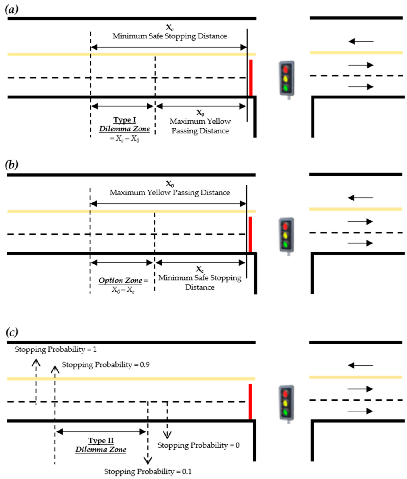[2,4]. The “dilemma zone,” also referred to as the “yellow phase dilemma zone,” is a critical area on a signalized intersection approach, where drivers can neither comfortably stop at the stop line nor proceed through the intersection during the yellow interval [5,6,7]. The presence of a dilemma zone, which is strongly affected by drivers’ behavior in the yellow interval, has a great effect on the safety level of a signalized intersection.

Driver behavior at signalized intersections in Greece has not been sufficiently researched yet. Taking into account that Greece continues to be among the worst performing countries in the EU with respect to road safety [8,9], studying driver behavior at signalized intersections could provide knowledge for targeted interventions in favor of road safety. It is pertinent to note that, the poor road safety performance in Greece is largely attributed to the aggressiveness of Greek drivers [2,9].

This paper deals with drivers’ choices to either stop or proceed through a signalized intersection when exposed to the yellow signal. The current research goes beyond the traditional data collection methods (observers, speed radars, scale drown on the road pavement, conventional videotaping), utilizing the emerging advancements of UAV (Unmanned Aerial Vehicles) technology, as well as the availability of video analysis and modeling software packages. In this context, the data required for the examination of drivers’ behavior were collected by videos captured from UAVs, which were then processed using a video analysis and modeling tool. This way, high accuracy time-based vehicle trajectory data were obtained and used for research purposes.

The main objective of the current research study is two-fold: Firstly, to model drivers’ stop/go behavior in the yellow interval at a signalized intersection, as a function of the various observable factors (distance to stop line, approaching speed and acceleration/deceleration at the onset of the yellow signal). In this respect, a binary choice model was developed, relating the probability of stopping or crossing as a function of the aforementioned factors. Emphasis was placed on the acceleration/deceleration factor. Secondly, to investigate the potential effect of drivers’ level of aggressiveness and relative position at the onset of the yellow signal on their stop/go behavior during the yellow phase. This way, potential differences in the probabilities of stopping or crossing the intersection could be identified, depending not only on the above-mentioned observable factors, but also on drivers’ aggressiveness and relative position. To this end, a latent class model was employed, which classified drivers into two groups (aggressive and non-aggressive), while a new variable—relative position—was calculated, indicating either drivers’ expected reaction/decision to stop or cross the intersection, or the existence of a dilemma or option zone. Finally, a new binary choice model was developed, which, in addition to the above-mentioned observable factors, also incorporated drivers’ aggressiveness and relative position as explanatory variables affecting their stop/go decision-making.

The rest of this paper is structured as follows: in Section 2, a brief description of the concept of dilemma zone is provided. In Section 3, a literature review is conducted, mainly focusing on studies that have dealt with acceleration/deceleration factor and drivers’ aggressiveness within the broader context of dilemma zone. Section 4 presents the research methodology, in relation to the data collection and preparation process, as well as the models’ development. Section 5 provides the results of the developed models, along with general sample statistics. Finally, Section 6 discusses those results and provide some conclusions in relation to the study.

2. Defining Dilemma Zone

Type I dilemma zone, the definition of which relies on the physical parameters of the situation (dilemma zone contributing factors form measurable physical characteristics), is inextricably linked to two distance-related factors: the minimum safe stopping distance (X_c) and the maximum yellow passing distance (X₀). For the calculation of X_c and X₀, the following equations are used, while constant parameter values are usually applied for perception/reaction times and acceleration/deceleration rates [2,5,10].

$$X_c=V_0{\delta }_{stop}+\frac{V_0^2}{2\ast a_{stop}},$$

(1)

$$X_0=V_0\mathsf{\tau }-\left(\mathrm{W}+\mathrm{L}\right)+\frac{1}{2}{a}_{pass}\ast {\left(\mathsf{\tau }-{\delta }_{pass}\right)}^2$$

(2)

where,

• V₀ is the vehicle’s approaching speed
• δ_stop is the perception/reaction time for safe stopping
• α_stop is the maximum deceleration rate for safe stopping
• δ_pass is the perception/reaction time for safe passing
• α_pass is the maximum acceleration rate for passing
• τ is the yellow time interval
• W is the width of the crossing road
• L is the typical vehicle length

When X_c > X₀, the distance between X_c and X₀ is defined as the type I dilemma zone. When X_c < X₀, the distance between X_c and X₀ is defined as the option zone. While a driver caught in the dilemma zone can neither comfortably stop before the stop line nor clear the intersection successfully, the option zone is an area where either stopping or crossing can be performed successfully [2,7].

The definition of the type II dilemma zone follows a purely probabilistic perspective: since the contributing factors of the type I dilemma zone (see Equations (1) and (2)) are difficult to be quantified and are usually assigned constant values (which can lead to inaccurate calculation of dilemma zone boundaries), the boundaries of the type II dilemma zone can be exclusively determined by drivers’ stopping probability [11]. More precisely, type II dilemma zone is an area on a signalized intersection approach, where more than 10% and less than 90% of drivers would choose to stop, in response to the yellow light indication [12,13,14,15]. In this context, distance or time to stop line are used as measures for the determination of type II dilemma zone boundaries [7]. Figure 1 illustrates the type I dilemma zone (a), option zone (b), as well as type II dilemma zone (c).

3. Literature Review

As it can be concluded from the previous sections, the existence of a dilemma zone, which is heavily affected by drivers’ behavior in the yellow phase, has a great effect on the safety level of signalized intersections. Such a critical area has attracted wide interest from researchers engaged in traffic engineering and safety, hence the issue of dilemma zone and drivers’ behavior in the yellow interval has been thoroughly examined over the last few decades. In their review paper, Shirazi and Morris [1] identified that such issues have attracted the greatest research attention among all objectives of intersection-related studies.

Most of the aforementioned studies explore the issue of dilemma zone from two perspectives: the accurate calculation of dilemma zone boundaries and the drivers’ stop/go behavior in the yellow interval, as a function of various factors.

The first group of studies sought to accurately determine dilemma zone boundaries, either by exclusively using the probability of stopping (type II dilemma zone) or by eliminating the static and the probabilistic definitions of type I and type II dilemma zone, by exploring the dynamic nature of its contributing factors. Following the probabilistic definition of type II dilemma zone, Zegeer and Deen [12] as well as Zegeer [13] defined dilemma zone as an area with a probability of stopping between 10% and 90% and calculated the distances corresponding to these probabilities for different vehicle speeds. Based on the same approach, several studies used distance and/or time to stop line as measures for the determination of type II dilemma zone boundaries [16,17,18,19,20,21,22,23]. On the other hand, few studies attempted to investigate the dynamic features of the contributing factors of the dilemma zone, namely, perception/reaction time and acceleration/deceleration rate [10,11,24,25,26].

The second group of studies focused on exploring the effect of various factors on drivers’ stop/go decision in the yellow interval. In this context, several types of models have been employed (binary logistic regression models, binary probit models, ordered probit models, agent-based behavioral models, fuzzy logic models, etc.) and various explanatory variables proved to significantly affect drivers’ stop/go behavior, including approaching speed, distance and time to stop line, yellow phase duration and signal cycle length, vehicle type, lane position, dilemma or option zone existence, red light camera presence, countdown timer existence, advance warning flashers existence, drivers’ age and gender, cell phone usage, etc. [2,22,27,28,29,30,31,32,33,34,35].

One of the main objectives of the current study is to examine the effect of acceleration/deceleration on drivers’ stop/go behavior in the yellow interval. To this end, the following literature is mainly focused on researches that dealt with the acceleration/deceleration factor.

Falling into the above-mentioned second group, several studies examined, among other variables, the effect of acceleration/deceleration on drivers’ stop/go decision making during the yellow phase. Amer et al. [36] followed a behavioral modeling approach to model drivers’ stop/go behavior in the yellow interval. The explanatory variables involved in the behavioral model included maximum accepted acceleration, maximum accepted speed, perception/reaction time, maximum accepted deceleration and error in the perceived distance to stop line. Biswas and Ghosh [37] employed different types of models, including a logistic regression model, an artificial neural network model, a fuzzy logic model and a weighted average hybrid model, with the overall aim of modeling drivers’ decision-making during the yellow phase. Distance and time to stop line, approaching speed and acceleration/deceleration rate were found to significantly affect drivers’ stop/go decision-making, for both vehicle types examined (cars and two-wheeled vehicles).

Li et al. [38] developed a sequential binary logit model to predict both drivers’ stop/go decision and red-light running violations during the yellow interval. Vehicle type, distance to stop line and approaching speed were found to be statistically significant factors affecting drivers’ stop/go behavior, while distance to stop line and acceleration appeared to be the contributing factors for red-light running violations. Sharma et al. [39] developed a dilemma zone hazard function to assess the probability of traffic conflict for a driver facing a yellow indication, on a high-speed signalized intersection. Even though the function developed was not binary, but rather a stochastic one, a binary probit model was initially employed to investigate the contributing factors for drivers’ stop/go decision. Having performed several iterations for the purpose of obtaining the best-fit probit model, required acceleration was found to be the instrumental variable affecting drivers’ stop/go decision process. Jahangiri et al. [40] used machine learning techniques, namely, Support Vector Machine (SVM) and Random Forest (RF), to predict red-light running violations. Research findings revealed that distance to stop line and required deceleration at the onset of the yellow signal, as well as average speed, maximum speed and standard deviation of acceleration for the monitoring period defined, were the factors that strongly affect red-light running violations.

It is pertinent to note that in all the above-mentioned studies, the acceleration/deceleration was not treated as a common factor employing the same methodology. More precisely, different measures of acceleration/deceleration were used, including acceleration/deceleration rate (estimated as the second derivative of the displacement-time relations), acceleration/deceleration at the onset of the yellow signal (calculated based on the observed instantaneous acceleration/deceleration at the initiation of the yellow signal), acceleration/deceleration during the yellow interval (measured two seconds after the initiation of the yellow light), required acceleration/deceleration (calculated as functions of distance to stop line, approaching speed, perception–reaction time and yellow signal duration), average acceleration/deceleration (based on mean value), maximum acceleration/deceleration (based on max value), etc.

Apart from the acceleration/deceleration factor, the current study also focuses on investigating the potential effect of drivers’ level of aggressiveness regarding their stop/go behavior during the yellow phase. As indicated by the relevant literature, such an issue has not yet been thoroughly examined, with only few studies having already sought to explore the relationship between drivers’ aggressiveness and stop/go decision in the yellow interval.

Papaioannou [2] used binary logistic regression to model the probability of stopping or crossing the intersection in the yellow interval, as a function of approaching speed, distance to stop line, drivers’ gender and age group, as well as the existence of dilemma zone. All the above-mentioned factors were proven to significantly affect drivers’ stop/go decision, with the existence of dilemma zone being the only exception. The study also proposed a two-step methodology for the classification of drivers based on their level of aggressiveness. More precisely, drivers were grouped into three categories (conservative, normal, aggressive), with the first criterion being their initial approaching speed and the second criterion being their behavior when exposed to the yellow signal (the latter being expressed by their stop/go decision related to the existence of a dilemma or option zone).

Elhenawy et al. [41] proposed a new predictor, namely, driver aggressiveness, to be integrated into the process of modeling drivers’ stop/run behavior at the initiation of the yellow signal. The calculation of the proposed parameter relies on historical data, with respect to drivers’ historical response to yellow indications. More specifically, the aggressiveness parameter is based on the number of runs that a driver has made during the yellow interval for a specific time period of monitoring, when the time to stop line was greater than the yellow signal duration and his/her approaching speed was equal or higher than the maximum posted speed limit. Using different machine learning techniques, namely, Adaptive Boosting (adaboost), Artificial Neural Networks (ANN) and Support Vector Machine (SVM), the study proved the ability of the -related to drivers’ aggressiveness- proposed predictor to further enhance the modeling of drivers’ stop/go behavior in the yellow interval.

Using machine learning techniques, namely, Support Vector Machines (SVM) and hidden Markov models (HMM), Aoude et al. [42] developed algorithms to classify drivers as compliant or violators, according to their behavior at signalized intersections. Various parameters were considered for the algorithm’s development, including approaching speed, acceleration, required deceleration and distance to stop line. The algorithms were successfully validated using intersection data and found to outperform the traditional drivers’ classification algorithms (time to intersection-based, required deceleration parameter-based and speed-distance regression-based).

Based on the literature review presented above, the contribution of the current research is the examination of acceleration/deceleration as well as drivers’ level of aggressiveness within the broader context of dilemma zone and the inclusion of these factors as potential predictors of drivers’ stop/go behavior at the yellow interval.

4. Materials and Methods

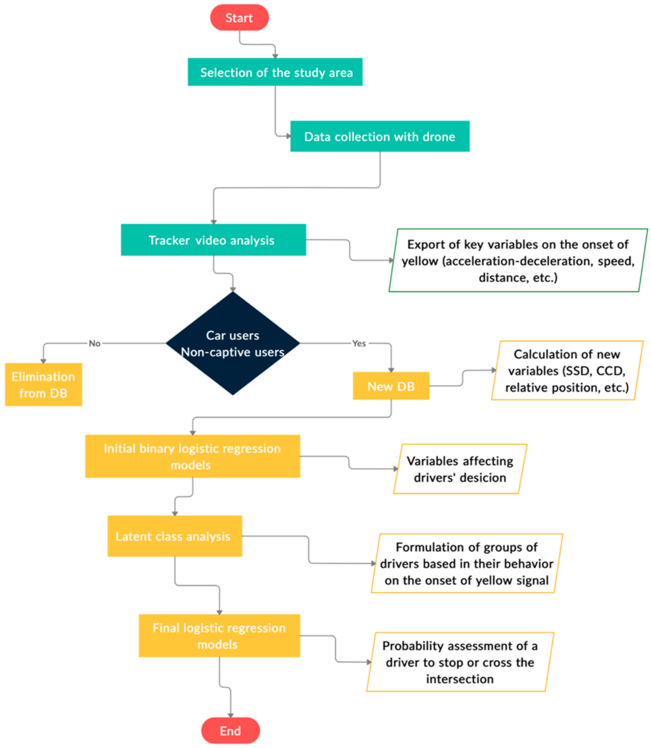
The purpose of this study is to examine driver’s behavior at a typical signalized intersection. This section presents the exact location of the intersection and outlines the general characteristics of the study area (intersection layout, traffic volumes, traffic signal time settings, etc.). The data collection process and analysis as well as the use of the appropriate statistical processing tools and techniques for modeling driver’s behavior are also presented in detail.

The entire methodological approach is briefly presented in the following Figure 2, while all the stages of the methodology are analyzed in detail in the following subsections.

4.1. Study Area

The research study was carried out at a signalized cross-shaped intersection located in eastern Thessaloniki, Greece. Traffic data were collected only for one approach of the intersection and more specifically the one that connects the city of Thessaloniki with the “Makedonia” airport, one of the major trip generators in the wider area of Thessaloniki. The chosen road section was functioning in good flow conditions, with a traffic flow of 1500 vehicles/hour and a capacity of 6000 vehicles/hour. This enabled the collection of adequate data, while the absence of saturation conditions could not affect the phenomenon under consideration. As the specific road section connects the city of Thessaloniki with an area of a mainly residential and recreational nature, it was considered that most drivers crossing the intersection are not in a hurry and therefore their driving behavior can be considered as representative for modeling driver’s behavior.

The study area was also selected in order to meet certain conditions. The specific intersection was selected because it consists of a single level without concave and convex slopes or without large vertical slopes in order to draw safe conclusions. In addition, in terms of video capture, the study area provided the ability to take video from an elevated location so that the recording angle is as sharp as possible to cover as large area as possible. Finally, the area was protected for UAV safe landing and take-off.

The signalization of the intersection gives priority to the direction towards the airport and has a significantly higher traffic load than the crossing road. The cycle length of the intersection under consideration was 85 s. The green signal duration was 50 s, the red 31 s and the yellow 4 s.

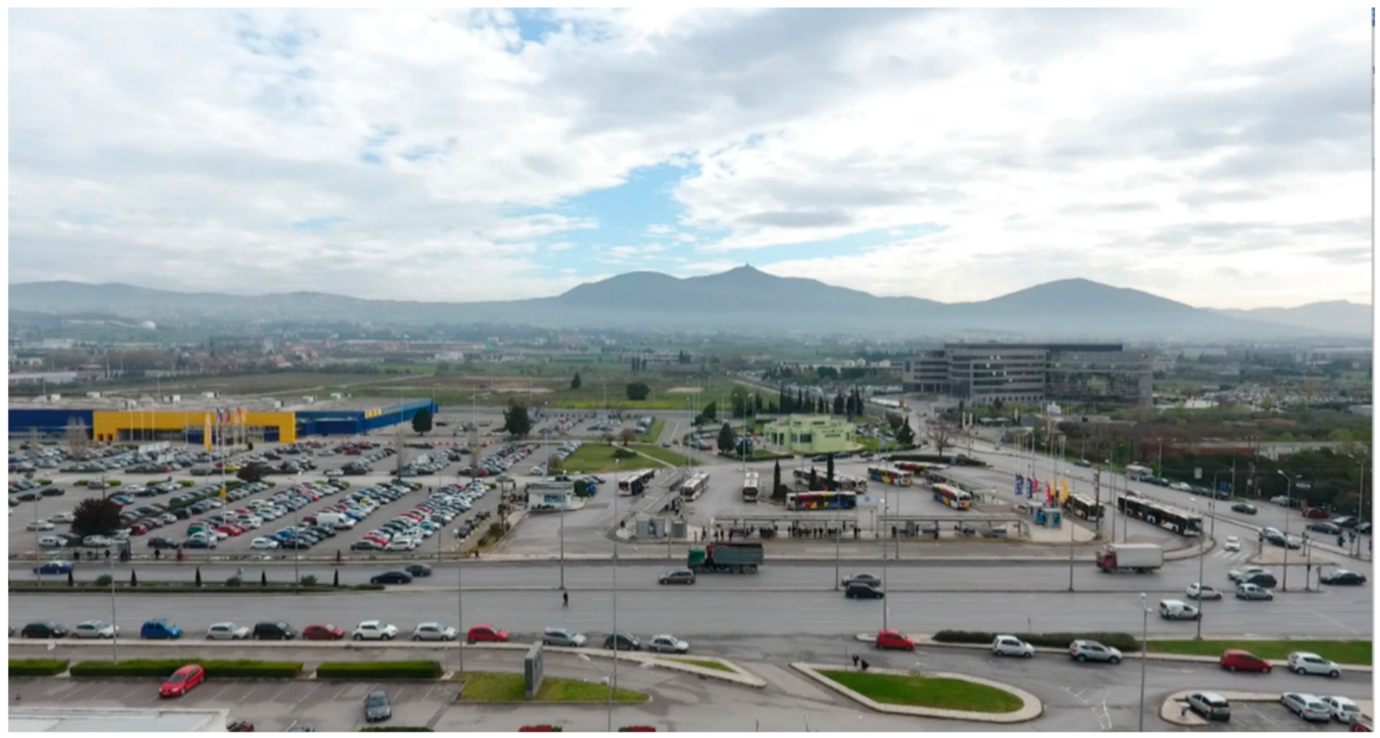
Figure 3 shows the study area, as captured by the UAV.

4.2. Data Collection

In order to adequately record the driving behavior within the dilemma zone, the necessary data were collected through video recordings captured by one UAV. The specific UAV had a built-in high-resolution camera and GPS and telecommunication equipment to transfer data to the ground station in real time.

Traditional methods of data collection have included measurements with observers or measurements with sensors placed in specific sections of the road. However, with the development of optical recording media, which is observed in recent years, the understanding of traffic phenomena can in several cases be carried out using video recordings of traffic characteristics and corresponding tracking procedures [11].

While UAVs were originally developed for military purposes and application, they have long been studied for other applications in various research fields including aerial photography, agriculture, product deliveries, policing and surveillance, etc. Cameras are standard equipment and are used for identifying and inspecting items or specific phenomena [43]. Numerous studies have been conducted to identify how UAVs can be used for transportation purposes in order to increase efficiency and safety, reduce costs and replace stationary systems [44].

Applications of UAVs on traffic monitoring can include several activities, such as identifying, tracking and monitoring specific vehicles, and several parameters can be extracted, such as densities, travel times, turning counts, queue lengths, etc. [45,46,47]. Several other studies focused on microscopic data and more specific phenomena, like detailed trajectory extraction and microscopic traffic parameters calculation [48]. Determining level of service (LOS), estimating average annual daily travel (AADT), measuring intersections operating conditions and creating origin destination flows can also be evaluated with the use of UAV [49,50,51]. Real-time visual data can be collected and used as input to improve existing traffic simulation models [52,53]. The use of advanced modeling and machine learning on videos captured by a UAV could provide useful traffic information, such as vehicle detection, traffic flow computation or vehicle classification [54]. Other studies have been focusing on the use of UAV for monitoring and analyzing traffic flow with respect to traffic safety [55,56].

Based on the above, UAVs constitute a more suitable means of capturing traffic measures than a fixed camera, as they provide the ability to film a larger area and deal with limitations, such as moving to any area to select the optimal location and avoiding points that prevent the complete recording of an object. Also, due to their relatively small size, they offer the possibility of recording traffic without being noticed by drivers. This is particularly important in the specific case where it concerns observations in the field of driver behavior, since in any other case, the driver can change his/her behavior, if he/she feels that it is being recorded or evaluated. In general, UAVs offer a more non-intrusive way of recording traffic phenomena.

Furthermore, due to the large height from which recording is made, data collection anonymity is secured, as no personal data such as vehicle registration plates or drivers’ personal data can be collected. This ensures the required data collection anonymity that should reflect a scientific data collection research. In addition, prior to the measurements carried out in the context of this work, flight plans were submitted to the legal control body for UAVs in Greece, the Civil Aviation Authority, and the necessary approval was given to carry out the relevant measurements. The official permission was required both for security reasons, due to proximity to the airport, as well as for privacy issues mainly related to sensitive personal data of people caught in video footage.

However, the UAVs have disadvantages in terms of battery life, resulting in limited flight time, while their flight depends on the current weather conditions, as it is not possible to use UAVs in case of rain and strong wind, for reasons of safety and protection of the equipment. Additionally, in the context of the present study, the high altitude from which the videos were recorded did not allow the collection of personal characteristics of users such as gender and age.

4.3. Data Analysis

The actual number of vehicles that were observed to face the yellow signal is equal to 617. Data were gathered for 12 days during March and April 2018. The total duration time of the collection period was 720 min.

For data analysis, a special kinematic analysis software was used in order to model and analyze the motion of objects from the collected videos. More specifically, the “Tracker Video Analysis and Modeling Tool” was used, an open-source software which provides tools for performing kinematic analysis of experimental video recordings. Features include position, speed, acceleration/deceleration tracking, multiple reference frames and model analysis (https://physlets.org/tracker/).

The specific software defines the so-called xa(t) paths (trajectories) i.e., the positions of each vehicle in time (t). If all vehicles in a road section are recorded in the same way, then the so-called “trajectory data” arises. This means that the resulting orbits and sizes are a function of only the coordinates (x, y) and the time variable t, of the object in question. Given the nature of their recording, trajectory data are the most detailed traffic data that can be collected and from which useful data can be obtained for the calculation of the dilemma zone.

The UAV video recording was set to 24 frames per second and the step size in the software used was set to 4 frames per second, resulting to six recordings for each second. This enabled the extraction of high-accuracy time-based data for each vehicle approaching the intersection, including:

• Approaching speed (from the onset of the yellow signal until the moment the vehicle stopped or passed the stop line)
• Distance to stop line (from the onset of the yellow signal until the moment the vehicle stopped or passed the stop line)
• Acceleration/deceleration (from the onset of the yellow signal until the moment the vehicle stopped or passed the stop line)
• Driver’s decision to stop or clear the intersection
• Type of vehicle
• The position of the vehicle in case a platoon is formed (Platoon leader, 1st or 2nd follower)

After the extraction of the above-mentioned information, a set of variables was calculated, including:

• Approaching speed (at the onset of the yellow signal)
• Average speed (between the initiation of the yellow signal and the moment the vehicle stopped or passed the stop line)
• Distance to stop line (at the onset of the yellow signal)
• Acceleration/deceleration (at the onset of the yellow signal and more precisely 0.5 s after the initiation of the yellow signal, for ensuring that perception/reaction time, assumed 1.5 s, has not elapsed)
• Average acceleration/deceleration (between the initiation of the yellow signal and the moment the vehicle stopped or passed the stop line)
• Existence of an approaching speed greater than the posted speed limit
• Categorization of drivers based on their behavior (if a driver stopped before or after the stop line, or if he/she crossed the intersection with yellow or red signal)

For further analysis and processing of data, it was decided to limit the original sample based on two specific conditions. Initially, it was decided to only analyze car drivers, since the other two categories of vehicles (heavy vehicles and motorcycles) constituted a very small percentage of the sample (5.3% and 3.2%, respectively). Only Platoon leaders were examined while exceptions were made only in the cases when Platoon leaders crossed the intersection and therefore the following drivers had a choice to cross or not. The third and subsequent drivers have very little chance of crossing the intersection without violating the red signal. In fact, only non-captive drivers were selected. The new sample included 525 vehicles.

The following variables were additionally calculated for the new sample:

• Calculation of safe stopping distance (SSD) and critical crossing distance (CCD) for all vehicles (based on type I dilemma zone Equations (1) and (2), and assuming constant values for perception/reaction time = 1.5 m/s² and maximum acceleration and deceleration rates = 3.5 m/s²)
• Calculation of vehicle’s relative position (based on the safe stopping distance (SSD), critical crossing distance (CCD) and the actual distance to stop line)

Table A1. Descriptive statistics of main scale variables.

Variable	Variable Coding	Description	Min	Max	Mean	Std. Deviation
Acceleration Deceleration Yellow (m/s2)	Acceleratio_Deceleration_Yellow	Measure of acceleration or deceleration on the yellow signal	−2.79	10.06	0.82	1.10
Average Speed (m/s)	Average_Speed	Average speed between yellow signal and stop line	2.81	34.73	19.23	7.07
Speed Yellow (m/s)	Speed_Yellow	Measure of speed on the yellow signal	3.92	32.95	20.60	4.21
Distance Yellow (m)	Distance_Yellow	Distance from stop line on the yellow signal	0.85	129.90	67.09	34.86
Average Acceleration Deceleration Rate (m/s2)	Average_Acceleration_Deceleration_Rate	Average acceleration or deceleration rate between yellow signal and stop line	−5.09	5.49	0.16	1.73
SSD (m)	SSD	Safe Stopping Distance	8.06	204.53	95.76	30.39
CCD (m)	CCD	Critical Crossing Distance	13.30	129.44	81.01	16.49

and

Table A2. Descriptive statistics of main nominal variables.

Variable	Variable Coding	Description	Range	Frequency
Category	Category	Classification of drivers based on their behavior	A: Stop	A: 32.10%
			B: Pass after stop line	B: 2.60%
			C: Pass with yellow	C: 57.70%
			D: Pass with red	D: 7.60%
Platoon Leader	Platoon_Leader	The first car in case of platoon on the onset of yellow	0: No	0: 28.80%
			1: Yes	1: 71.20%
1st Follower	1_Follower	The second car in case of platoon on the onset of yellow	0: No	0: 77.30%
			1: Yes	1: 22.70%
2nd Follower	2_Follower	The third car in case of platoon on the onset of yellow	0: No	0: 93.80%
			1: Yes	1: 6.20%
Decision	Decision	Decision to stop or pass the stop line	0: Stop	0: 34.70%
			1: Pass	1: 65.30%
Decision Previous	Decision_Previous	Decision to stop or pass the stop line of previous car (for 1st and 2nd followers only)	0: Stop	0: 12.40%
			1: Pass	1: 87.60%
Change Lane	Change_Lane	Change lane between the onset of the yellow signal and the stop line	0: No	0: 98.10%
			1: Yes	1: 1.90%
Greater than Speed Limit	Greater_than_Speed Limit	The speed on yellow signal is above 70 km/h	0: No	0: 33.70%
			1: Yes	1: 66.30%
Acceleration	Acceleration	Acceleration or deceleration after the onset of the yellow signal	0: No	0: 35.40%
			1: Yes	1: 64.60%
Relative Position	Rel_Position	Vehicle’s relative position, speed and acceleration on the onset of the yellow signal	1: Obvious Decision Stop	1: 31.20%
			2: Option Zone	2: 0.60%
			3: Dilemma Zone	3: 9.30%
			4: Obvious Decision Pass	4: 58.90%
Type of vehicle	Type_of_vehicle	Type of vehicle	1: Car	1: 91.40%
			2: Truck	2: 5.30%
			3: Moto	3: 3.20%

For the binary variables entered in the latent class model, “1” and “2” values were used for “Yes” and “No”.

in the Appendix A section, present the descriptive statistics for the scale and nominal variables, respectively, used further in the data analysis.

4.4. Modeling Drivers’ Behavior

When examining drivers’ behavior at signalized intersections, a high number of factors need to be examined. Moreover, as indicated by the pertinent literature, several modeling approaches have already been employed. In this section, the factors examined for the current research purposes, as well as the models’ preparation processes are presented.

4.4.1. Formulation of Initial Binary Logistic Model

Drivers who face the yellow signal have two distinct choices, to stop or clear the intersection. Thus, a binary logistic regression model could be used for explaining drivers’ behavior as a function of various observable factors. The variables tested for inclusion in the model, are the following:

• Approaching speed (both at the onset of the yellow signal and average)
• Distance to stop line
• Acceleration/deceleration (both at the onset of the yellow signal and average)
• Other potential explanatory variables, including drivers’ position in the platoon (platoon leader, 1st and 2nd follower), lane change, etc.

The description and coding of all variables tested in the model, are presented in Table A1 and Table A2 at the Appendix A. The dependent variable has been driver’s decision, taking values 0 and 1. Zero (0) stands for stopping and one (1) for crossing the intersection. Different combinations of explanatory variables were tested. The form of the model is given by the following Equation [57]:

$${\mathrm{P}}_{\mathrm{i}}\left(\mathrm{stop}\right)=\frac{1}{1+{\mathrm{e}}^{-{\mathrm{z}}_{\mathrm{i}}}}$$

(3)

where,

• P_i is the probability of the ith case to stop
• Z_i is the result of a linear function of the various factors (explanatory variables)

The selection of the best-fit binary choice model requires an assessment of the good adaptation of the model. The statistical tests carried out in order to evaluate the statistical significance of the model, were the following:

• The Nagelkerke R Square index, which gives an indication of the size of the sample variance that is ultimately interpreted by the regression. The closer to 1 is the value of this indicator, the better the model adapts to the sample data.
• Hosmer and Lemeshow test has been also used to check the proper adaptation of the sample data. Values of sig.> 0.05 at significance level a = 95% indicate that the model is well adapted to the data.
• Another measure of the good adaptation of the model is the SPSS Classification Table, which compares the observed probabilities with those provided for by the model. The higher the percentage of cases of the dependent variable correctly predicted based on the model, the better the model adjustment [57].

4.4.2. Formulation of Latent Class Model

Latent Class Analysis (LCA) is a technique for the analysis of clustering among observations in multi-way cross-classification tables of categorical variables, being usually employed to investigate sources of confounding between the observed variables, as well as to identify and characterize clusters of similar behaviors [58,59]. The main objective of LCA is to fit a latent class model in which any confounding between the observed—also called manifest—variables can be explained by a single, unobserved—also called latent—variable. For the study purposes, the aforementioned latent variable is assumed to be drivers’ aggressiveness. Based on the values of the manifest variables, the latent class model probabilistically groups each observation into a latent class and, thus, the initial dataset is finally segmented into several exclusive subsets (latent classes). This grouping produces expectations about the way that each observation will respond on each of the observed manifest variables [59]. The basic latent class model is given by the following equation [60], while a more detailed definition of LCA and its mathematical background can be found in Linzer and Lewis [59] and Hagennars and McCutcheon [61].

$$\mathrm{P}\left(\left.{\mathrm{y}}_{\mathrm{n}}\right|\mathsf{\theta }\right)={{\displaystyle \sum }}_1^{\mathrm{s}}{\mathsf{\pi }}_{\mathrm{j}}{\mathrm{P}}_{\mathrm{j}}\left(\left.{\mathrm{y}}_{\mathrm{n}}\right|{\mathsf{\theta }}_{\mathrm{j}}\right)$$

(4)

where,

• y_n is the nth observation of the manifest variables
• S is the number of classes
• π_j is the prior probability of membership in class j
• P_j is the class specific probability of y_n given the class specific parameters θ_j
• θ_j are the class specific parameters

The manifest variables which were taken into account for the development of the latent class model, included approaching speed, acceleration/deceleration at the initiation of yellow signal, drivers’ position in the platoon (three variables for platoon leaders, first and second followers, where one (1) stands for belonging and two (2) for not belonging in each position) and a variable indicating whether the approaching speed was greater than the posted speed limit or not (where one (1) stands for speeds greater than speed limit and two (2) for speeds lower than speed limit). The former two factors (approaching speed and acceleration/deceleration) were the major variables of interest, while the latter were used primarily for avoiding identifiability issues. Given the fact that approaching speed and acceleration/deceleration were continuous variables in the initial dataset, a recoding was performed to categorize all manifest variables entered the latent class model. In respect to the acceleration/deceleration recoding, several studies have already proposed different typical values for the determination of the normal/acceptable acceleration/deceleration rates [62]. For the study purposes, the normal deceleration/acceleration values are assumed to range between −0.9 m/s² and +0.9 m/s². The thresholds used for the approaching speed and acceleration/deceleration recoding are presented in

Table 1. Thresholds for approaching speed and acceleration/deceleration recoding.

Variable Initial Coding	New Recoded Variable	Recoding Thresholds	Recoding Values	Interpretation
Speed_Yellow	Speed_Yellow_Recoded	Speed_Yellow ≤ 60 km/h	1	Low Approaching Speed
		60 km/h < Speed_Yellow ≤ 70 km/h	2	Medium Approaching Speed
		70 km/h < Speed_Yellow ≤ 80 km/h	3	High Approaching Speed
		Speed_Yellow > 80 km/h	4	Very High Approaching Speed
Acceleration_Deceleration_ Yellow	Acceleration_Deceleration_Yellow_Recoded	Acceleration_Deceleration_Yellow < −0.9 m/s2	1	High Deceleration
		0.9 m/s2 ≥ Acceleration/Deceleration_Yellow ≥ −0.9 m/s2	2	Medium Deceleration/Acceleration
		Acceleration_Deceleration_Yellow > 0.9 m/s2	3	High Acceleration

.

After inserting all the above-mentioned manifest variables, several latent class models with various numbers of classes were developed. As shown in

Table 2. Changing values of Bayesian Information Criterion (BIC) by varying number of classes.

Number of Latent Classes	BIC
2	3714.978
3	3441.026
4	3332.407
5	3290.169
6	3312.328

, the changing values of model fit statistics by varying number of classes, in terms of the Bayesian Information Criterion (BIC), indicated that the 5-class model (bold text) was the best-fit one, having the lowest BIC value.

In fact, the selection of the best-fit latent class model forms a complex issue, since there is not a commonly accepted statistical indicator for choosing the appropriate number of latent classes [63]. In this context, apart from the BIC criterion, a wide number of methods have been proposed for the optimal class selection, including Akaike Information Criterion (AIC), consistent Akaike Information Criterion (cAIC), adjusted Bayesian Information Criterion (aBIC), Bootstrap likelihood ratio test (BLRT), entropy, high enough class population shares and, finally and above all, conceptual and interpretable meaning [64]. Based on the above, the 2-class model was proved to be the best-fit one and chosen for drivers’ classification according to their aggressiveness.

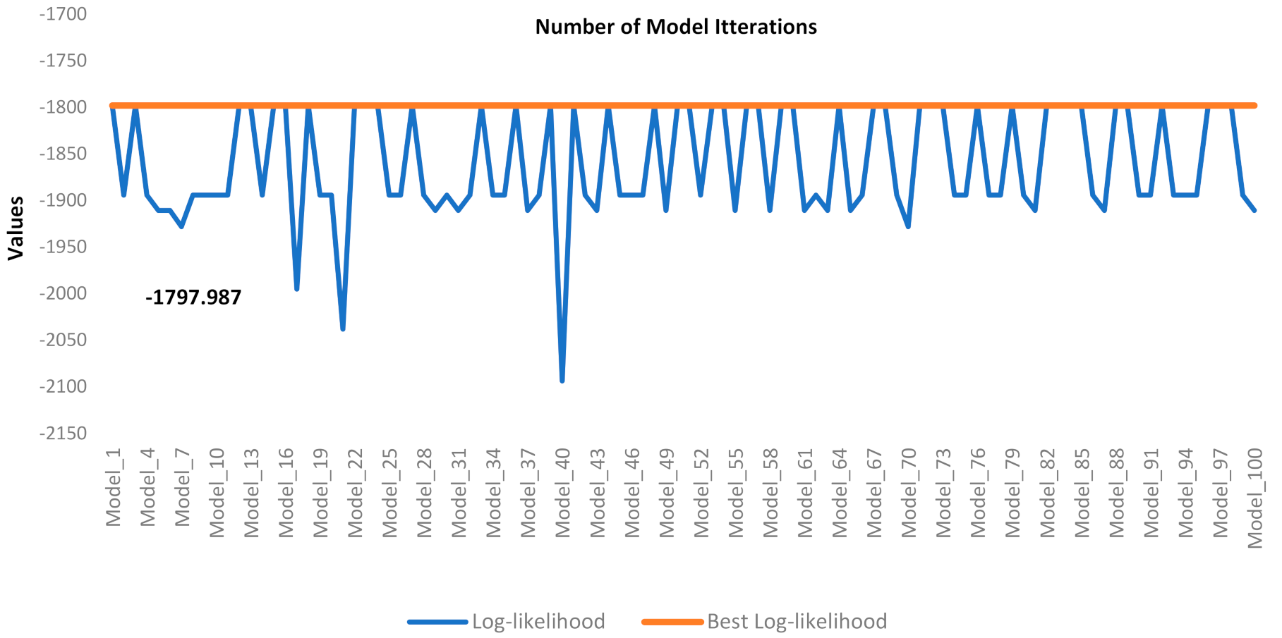
It should also be noted that the EM algorithm, which is commonly used by the LCA software packages, depending on the initial parameter values chosen in the first iteration, may only find a local rather than the global, maximum of the log-likelihood function [59]. This fact may lead to different classification results in each model run. To avoid local maxima, the latent class model was specified, in terms of programming language, using the appropriate argument. Consequently, the latent class model was automatically estimated one hundred (100) times using different initial parameter values and the model with the greatest value of the log-likelihood function was finally chosen. The local and global maximum log-likelihoods in all the attempts at fitting the model, are shown in Figure 4. For the 2-class model, the global maximum log-likelihood of −1797.987 was found in the first attempt at fitting the model.

4.4.3. Formulation of Final Binary Logistic Model

After the development of the latent class model, which classified drivers into groups based on their aggressiveness, binary logistic regression models were recalculated. The main difference between the new models and the initial ones is that additional variables related to the aforementioned drivers’ categorization (aggressive/non-aggressive) and variables indicating drivers’ expected reaction/decision to stop or cross the intersection related to the vehicles’ relative position (dilemma zone, option zone, obvious decision stop, obvious decision pass) were used.

For the new “relative position” variable, three (3) dummy variables were constructed (“obvious_decision_stop”, “option_zone”, “dilemma_zone”) and the reference category was set as “obvious_decision_pass”. The relevant results of all the above statistical analysis methods and tools, are presented in the following section.

5. Results

5.1. Sample Statistics

The actual number of vehicles that were observed to face the yellow signal was equal to 617. The largest proportion of the sample consisted of cars (91.40%) while heavy vehicles and motorcycles account for 5.30% and 3.20% of the sample, respectively. Platoon leaders make up for 71.20% of the sample, 1st followers 22.70% of the sample and 2nd followers 6.20% of the sample. A total of 65.30% of the sample facing the yellow signal decided to pass while, with regards the categorization of drivers on the basis of their decision, it appears that more than 57% of the sample crossed the intersection during the yellow indication whereas about 32% of the sample decided to stop. A small percentage of the sample (2.60%) stopped shortly after the stop line while almost 8% of the sample crossed the intersection with red signal, thus demonstrating a relatively dangerous driving behavior. Another characteristic of potential dangerous driving behavior is the fact that more than 66% of the sample move at a higher speed than permitted as the average speed of drivers at the time they faced the yellow signal was 20.60 m/s (S.D = 4.21) or 74.16 km/h, slightly higher than the posted speed limit (70 km/h). Almost 2% of the sample decided to change lanes from the moment they faced the yellow signal until they approached the stop line.

The average distance from speed line was calculated to 67.09 m (S.D. = 34.86). The average acceleration when facing the yellow signal was 1.09 m/s2 (S.D. = 0.96) whereas the average deceleration rate was 0.63 m/s2 (S.D. = 0.62).

Table 3. Descriptive statistics of main variables based on drivers’ behavior.

Variable	Description	Behavior	Mean	Std. Deviation	Minimum	Maximum
Distance (m)	Distance from stop line at the onset of the yellow signal	Stop	97.14	21.78	39.06	128.90
		Go	48.39	23.89	6.55	104.10
		Passed with red	95.80	16.81	61.15	127.90
		Stop after stop line	86.54	18.69	61.32	125.70
Speed (m/s)	Approaching speed at the onset of the yellow signal	Stop	17.66	3.59	3.92	27.37
		Go	22.65	3.40	11.81	32.95
		Passed with red	20.59	3.07	12.81	26.34
		Stop after stop line	18.91	3.26	13.35	25.10
Acceleration/Deceleration (m/s2)	Acceleration/Deceleration at the onset of the yellow signal	Stop	0.27	0.87	−2.52	2.72
		Go	1.13	1.13	−2.00	10.06
		Passed with red	0.94	0.70	−0.18	2.92
		Stop after stop line	0.14	1.24	−2.79	1.34

presents the mean, standard deviation, minimum and maximum values of distance to stop line, approaching speed and acceleration/deceleration at the onset of the yellow signal, based on drivers’ behavior approaching the intersection.

As previously mentioned, it was decided to limit the original sample to only car users and non-captive users (Platoon leaders and 1st or 2nd followers only if the lead driver crossed the intersection and therefore the following drivers had a choice to do the same). For the new sample (525 vehicles recorded) additional variables were calculated such as safe stopping distance (SSD) and critical crossing distance (CCD) as well as calculation of vehicle’s relative position based on distance from stop line, speed and acceleration/deceleration on the onset of the yellow signal. Based on these calculations, almost 60% of the drivers were found to be in an obvious decision pass zone, more than 31% were found to be in an obvious decision stop zone while about 9% of the sample were in a dilemma zone.

Classification of drivers into a specific position indicates the decision a driver should make based on specific characteristics (distance, speed, acceleration/deceleration) at the initiation of the yellow phase. For example, a driver who is classified in the obvious decision to stop zone based on his/her behavior at the start of the yellow signal, should stop. However, this is not always the case, as demonstrated in

Table 4. Driver’s decision based on their relative position.

Decision	Dilemma Zone	Obvious Decision Pass	Obvious Decision Stop	Option Zone
Stop	36.73%	4.85%	86.59%	66.67%
Pass	63.27%	95.15%	13.41%	33.33%

, which presents the percentage of “expected action” of drivers based on the decision they should make in relation to the relative position to which they belong.

The table above shows that about 5% of drivers decide to stop when they can cross safely the intersection while about 13% of the sample decides to cross the intersection where, based on their position, speed and acceleration/deceleration, they should have stopped. As regards the dilemma zone and the option zone, there is no question of following the expected action, as in these specific zones driver’s decision cannot be predetermined.

Independent-samples t-tests were conducted to compare speed, distance and acceleration/deceleration of approaching vehicles on the onset of the yellow signal for drivers who followed or not the predetermined decision (expected action).

For drivers belonging to the obvious decision pass zone, there was a significant difference between the mean speed of vehicles the drivers of which acted as expected (M = 22.81, SD = 3.36) and those who did not (M = 19.08, SD = 2.86); t (16) = −4.89, p = 0.000. For drivers belonging to the obvious decision stop zone, there was a significant difference between the mean speed of vehicles the drivers of which acted as expected (M = 17.11, SD = 3.38) and those who did not (M = 18.91, SD = 2.82) conditions; t (31) = −2.71, p = 0.01. For drivers belonging in the dilemma zone, as there is no standard decision, there was a significant difference between the mean acceleration of vehicles who passed the intersection (M = 1.01, SD = 0.81) and those who stopped (M = −0.27, SD = 0.93) conditions; t (32) = −4.89, p = 0.00.

For drivers who decided to pass the intersection, there was a significant difference between the mean speed of vehicles that belong to the obvious decision to stop zone (M = 18.93, SD = 2.88) and those who belong to the obvious decision to pass zone (M = 22.81, SD = 3.37) conditions; t (24) = −5.87, p = 0.000. There was also a significant difference between the mean distance to stop line of vehicles that belong to the obvious decision to stop zone (M = 96.84, SD = 21.68) and those who belong to the obvious decision to pass zone (M = 46.57, SD = 22.78) conditions; t (23) = 10.23, p = 0.000.

5.2. Initial Binary Logistic Regression Model Results

This section presents the results of the binary logit choice model that has been developed within the framework of the study.

Table 5. Parameter estimates of the initial binary choice model.

Variable	Estimate	Std. Error	p-Value	OR
Speed_Yellow	0.72	0.09	0.00	2.06
Distance_Yellow	−0.11	0.01	0.00	0.89
Acceleration_Deceleration_Yellow	1.92	0.28	0.00	6.79
Constant	−5.59	1.26	0.00	0.00
Goodness of Fit Metrics
Nagelkerke R Square	0.83
Hosmer and Lemeshow Test	0.81
Classification (overall percentage)	91.40%

illustrates the parameter estimates of the binary choice model, as well as the results of the relevant static tests to estimate the model’s goodness to fit. The odds ratio (OR) were also calculated for the specific binary choice model. An odds ratio is a relative measure of effect, which allows the comparison of a change in one variable to the outcome of the model. It should also be noted that for the formulation of the binary logistic regression model, non-captive users were used (Platoon leaders and 1^st or 2^nd followers only if the lead driver crossed the intersection and, therefore, the following drivers had a choice to do the same).

As shown in the Table above, the most important parameters that affect drivers’ stop/go decision are the distance of the approaching vehicle to the stop line, the approaching speed and the acceleration/deceleration at the onset of yellow signal, with the latter having the greatest influence on the final decision. More specifically, the odds ratio for the acceleration/deceleration at the onset of yellow signal is 6.79, indicating that those who travel with higher acceleration rates are on average 6.79 times more likely to pass than those who choose to travel with lower acceleration or deceleration rates.

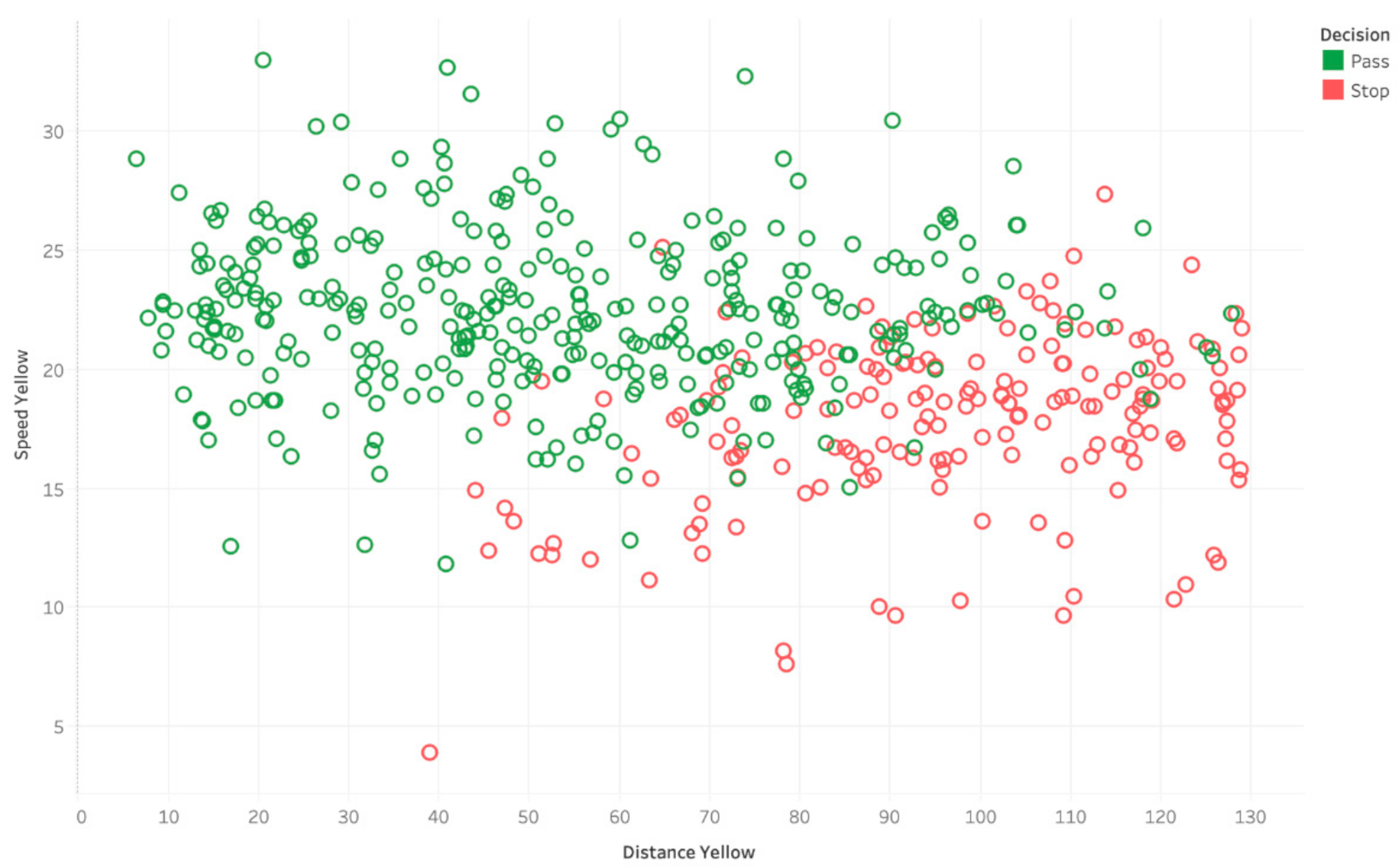
According to Figure 5, for vehicles close to the stop line, up to 60 m, the decision to pass is made regardless of the speed. The opposite applies for distances greater than 100 m, as drivers mostly decided to stop. In the intermediate zone between 60 m and 100 m, speed plays a vital role in driver’s decision. It seems that a speed of approximately 20 m/s is what mainly influences whether the driver will decide to pass or not. Most drivers in vehicles with higher speeds choose to cross the intersection. Distance from stop line also plays an important role, as the greater the distance from the stop line, the less likely a vehicle is to cross the intersection during the yellow light. Attention should also be paid to the fact that the critical distance to the stop line, based on Figure 5, is between 80 m and 90 m.

Independent-samples t-tests were conducted to compare speed, distance and acceleration/deceleration of approaching vehicles on the onset of the yellow signal for drivers who chose to pass or stop at the stop line. Distance, speed and acceleration/deceleration of approaching vehicles were found to be significantly different between the two groups of drivers. More specifically, the speed of drivers who chose to pass was systematically faster (M = 22.43, SD = 3.42) than the speed of drivers who stopped at the stop line (M = 17.73, SD = 3.57) conditions; t (340) = −14.41, p = 0.00. For drivers who passed the intersection, the mean acceleration was higher (M = 1.11, SD = 1.09) compared to those who stopped (M = 0.26, SD = 0.89) conditions; t (421) = −9.56, p = 0.00. Distance from stop line was also found to be significantly different between drivers who passed (M = 53.56, SD = 27.52) and drivers who stopped (M = 96.48, SD = 21.70) conditions; t (434) = 19.51, p = 0.00.

Based on the above, it can be concluded that the probability to stop or clear the intersection is mainly correlated to speed, distance and acceleration/deceleration of an approaching vehicle on the onset of the yellow signal. While distance from stop line may be considered as a random parameter, as no one can predict the distance between the vehicle and the stop line at the onset of the yellow signal, the speed and acceleration/deceleration can be considered as parameters that are mainly affected by driver’s behavior. As it can also be seen in Figure 6, drivers who chose to pass are mainly correlated with higher speeds and acceleration rates. On the contrary, drivers who chose to stop are mainly correlated with lower speeds and lower acceleration and deceleration rates. These two parameters, speed and acceleration/deceleration rate, that are strongly associated with driver’s decision are used in the next step to classify drivers in terms of aggressiveness, based on their behavior. For example, an aggressive driver can be found driving with higher speeds (maybe higher than speed limits) and acceleration rates compared to a conservative driver who would mainly choose to drive at lower speeds and exercise lower acceleration rates.

After the development of the initial binary choice model, further research was conducted with the overall aim of identifying potential differences in the probabilities of stopping or crossing the intersection, depending not only on the observable factors of approaching speed, distance to stop line and acceleration/deceleration, but also on drivers’ level of aggressiveness and their relative position at the initiation of the yellow signal. To this end, a latent class model was employed for drivers’ classification based on their aggressiveness and a new variable—relative position—was calculated, indicating either drivers’ expected response to the yellow signal or the existence of a dilemma or option zone. Finally, the initial binary choice model was further enriched, incorporating—in addition to the above-mentioned observable factors—drivers’ aggressiveness and relative position as potential contributing factors to their stop/go decision. The results of the latent class model and the final binary choice model are presented in the following sections.

5.3. Latent Class Analysis Results: Driver Classification according to Aggressiveness

In this section, the results of the latent class model developed to classify drivers according to their aggressiveness are presented.

Table 6. Conditional item response (column) probabilities by outcome variable for each class (row).

Speed_Yellow_Recoded
	Pr(1)	Pr(2)	Pr(3)	Pr(4)
Class_1	0.0000	0.0000	0.4454	0.5546
Class_2	0.4011	0.5989	0.0000	0.0000
Acceleration_Deceleration_Yellow_Recoded
	Pr(1)	Pr(2)	Pr(3)
Class_1	0.0287	0.5057	0.4655
Class_2	0.0282	0.7119	0.2599
Platoon_Leader
	Pr(1)	Pr(2)
Class_1	0.7414	0.2586
Class_2	0.6610	0.3390
1st_Follower
	Pr(1)	Pr(2)
Class_1	0.2184	0.7816
Class_2	0.2542	0.7458
2nd_Follower
	Pr(1)	Pr(2)
Class_1	0.0374	0.9626
Class_2	0.0847	0.9153
Greater_than_Speed_Limit (Approaching Speed)
	Pr(1)	Pr(2)
Class_1	1	0
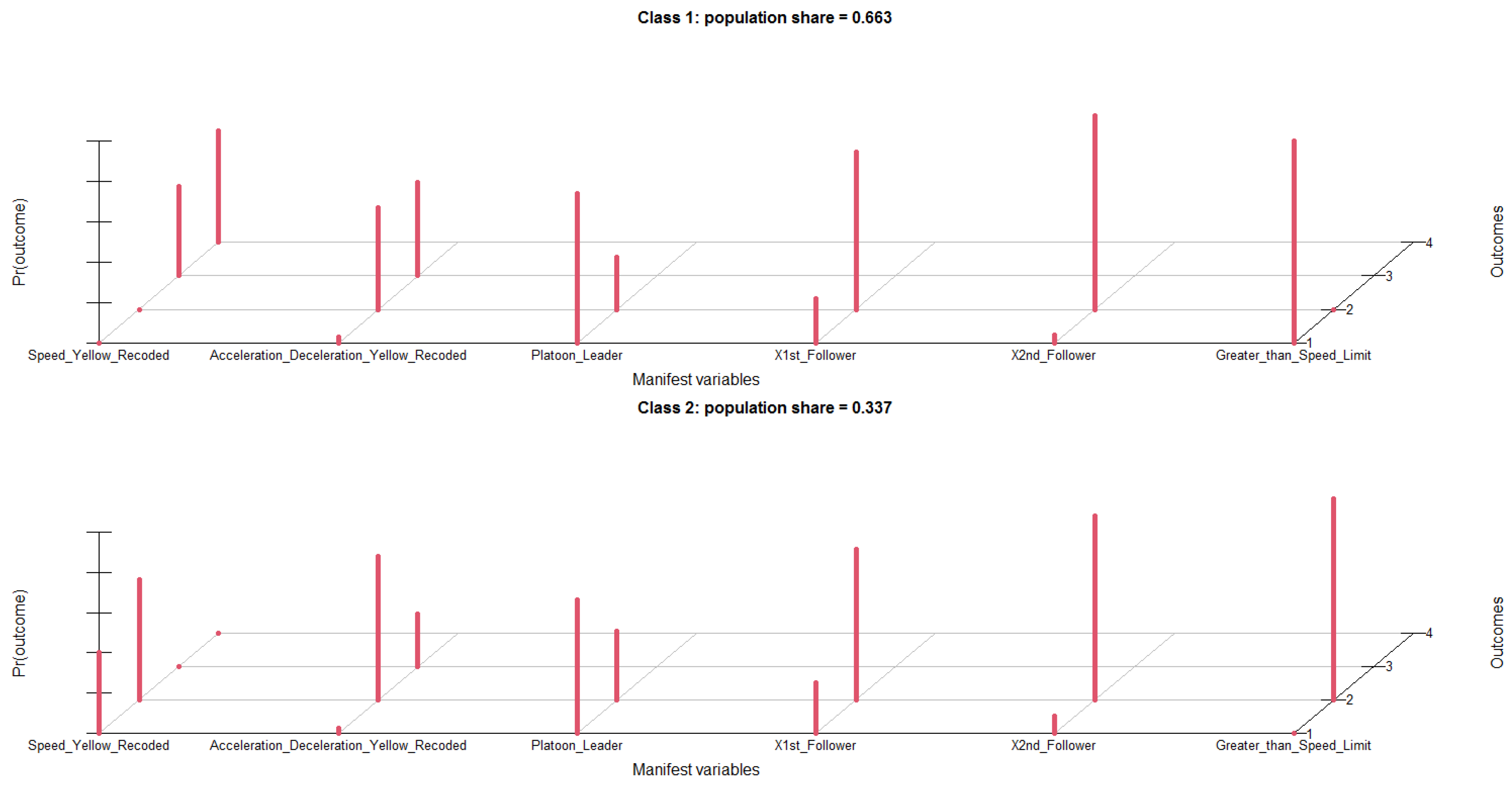
Class_2	0	1

shows the estimated class-conditional response probabilities. These probabilities are reported for all manifest variables, with each row corresponding to a latent class and each column corresponding to a category of each manifest variable (see recoding values in Table 1 i.e., 1st column of speed_yellow_recoded: low approaching speed, 2nd column of speed_yellow_recoded: medium approaching speed, 3rd column of speed_yellow_recoded: high approaching speed, etc.).

Based on the latent class model results, the two (2) estimated latent classes have conceptual and interpretable meaning, with class_1 representing the aggressive drivers and class_2 representing the non-aggressive drivers. Since the manifest variables were entered in the latent class model as integers, the columns of the above table show the probabilities of observing a response of 1, 2, (3, 4) for each manifest variable, conditional on a driver being assigned to latent classes 1 (“aggressive”) or 2 (“non-aggressive”). Thus, a driver belonging to the first “aggressive” class, has a 45% and 55% chance of approaching the intersection with high and very high speed, respectively, and a 0% chance of approaching the intersection with medium or low speed. Along the same lines, a driver belonging to the first “aggressive” class, has a 50% and 47% chance of approaching the intersection with medium deceleration/acceleration rate and high acceleration rate, respectively, while a driver belonging to the second “non-aggressive” class, has a 71% and 26% chance of approaching the intersection with medium deceleration/acceleration rate and high acceleration rate, respectively. Lastly, a driver belonging to the first “aggressive” class, has a 100% chance of approaching the intersection with a speed greater than the posted speed limit, while a non-aggressive driver has a 100% chance of approaching the intersection with a speed lower than the speed limit. The variables regarding drivers’ position in the platoon are not further discussed, since they have been used mostly for avoiding identifiability problems.

Table 7. Estimated class population shares and predicted class memberships (by modal posterior prob.).

Estimated Class Population Shares
Class_1	Class_2
0.6629	0.3371
Predicted Class Memberships (by Modal Posterior Prob.)
Class_1	Class_2
0.6629	0.3371

provides the estimated mixing proportions corresponding to the share of observations belonging to each latent class (estimated class population shares). An alternative method for the determination of the size of the latent classes is to assign each observation to a latent class on an individual basis, according to its modal posterior class membership probability. These values are also provided in the following table (predicted class membership by modal posterior probability). Both the estimated class population shares and the estimated class-conditional response probabilities that have already been shown in Table 6, are presented in Figure 7.

As shown in Table 7, there is a perfect congruence between the two above-mentioned sets of population shares, indicating a good fit of the latent class model to the observed data. Moreover, it is pertinent to note that the latent class model classified drivers into aggressive (66%) and non-aggressive (34%), indicating that most drivers approaching the intersection exercised an aggressive behavior. This fact is in line with the findings of Papaioannou [2], who modeled driver stop/go decision at the yellow interval in another signalized intersection in Thessaloniki, Greece.

Finally,

Table 8. Latent class model goodness-of-fit statistics.

Fit for 2 Latent Classes:

number of observations: 525

number of estimated parameters: 19

residual degrees of freedom: 172

maximum log-likelihood: −1797.987

AIC(2): 3633.973

BIC(2): 3714.978

G^2(2): 669.3934 (Likelihood ratio/deviance statistic)

X^2(2): 725.9775 (Chi-square goodness of fit)

presents some more information regarding the latent class model developed, as well as a number of goodness-of-fit statistics.

5.4. Final Binary Logistic Regression Model Results

Based on the results of the latent class analysis, drivers were classified into two groups: aggressive and non-aggressive. Subsequently, the proposed classification of drivers was used in order to formulate a new binary logistic regression model, which contained not only physical variables, such as approaching speed, distance to stop line and acceleration/deceleration, but also variables related to drivers’ aggressiveness, as well as vehicles’ relative position at the onset of the yellow signal (dilemma zone, option zone, obvious decision to pass, obvious decision to stop).

Table 9. Parameter estimates of the final binary choice model.

Variable	Estimate	Std. Error	p-Value	OR
Acceleration_Deceleration_Yellow	1.72	0.25	0.00	5.56
Distance_Yellow	−0.05	0.01	0.00	0.95
Obvious_Decision_Stop	−3.09	0.60	0.00	0.05
Option_Zone	−3.46	1.38	0.01	0.03
Dilemma_Zone	−1.10	0.56	0.05	0.33
Observed_LCA_Classification	1.92	0.46	0.00	6.80
Constant	3.68	0.70	0.00	39.70
Goodness of Fit Metrics
Nagelkerke R Square	0.81
Hosmer and Lemeshow Test	0.34
Classification (overall percentage)	91.00%

illustrates the parameter estimates of the final binary choice model, as well as the results of the relevant statistical tests to estimate the model’s goodness to fit. The variable related to vehicles’ relative position (“rel_position”) was recoded in three dummy variables, namely, “Obvious_Decision_Stop”, “Option_Zone” and “Dilemma_Zone”, while the reference category was “Obvious_Decision_Pass”.

Based on the results presented in Table 9, the probabilistic power of the model is considered quite good. Nagelkerke R Square is 0.81 indicating that the model adapts well to the sample data. The overall classification that compares the observed data with the predicted probabilities provided by the model, indicates that the specific model correctly predicts 91% of the cases which correspond to a good adaption of the model to the sample data. The most important parameters, based on the odds ratio of the variables (OR column), that influence the driver’s decision as to whether to pass or stop, are the distance of the approaching vehicle from the stop line and acceleration/deceleration at the time of the yellow signal. These parameters were also used in the initial binary logistic regression model.

The main difference between the final and the initial model is that the new model includes variables related to the driver’s behavior as well as the existence or not of a dilemma zone. In the new model, as shown by the comparison of odds ratio, the greatest influence on the final decision has the categorization of drivers based on their behavior. Aggressive drivers are almost seven times more likely to cross the intersection than more conservative drivers irrespective of their relative position. Acceleration continues to have a major impact on the final decision as well as on the original model. Also, those drivers who are in a dilemma zone are less likely to cross the intersection. It should be noted here that the variable acceleration/deceleration at the onset of the yellow signal was also used as input variable for the LCA classification of drivers. With the use of Spearman’s correlation test, it was found that there was no statistically significant correlation between acceleration/deceleration and the observed LCA classification (r_s = 0.230).

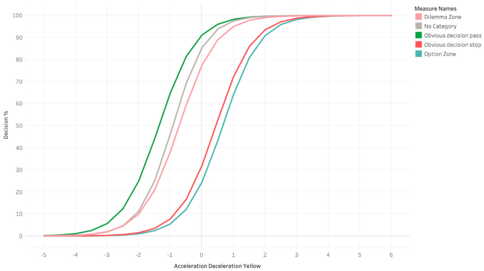
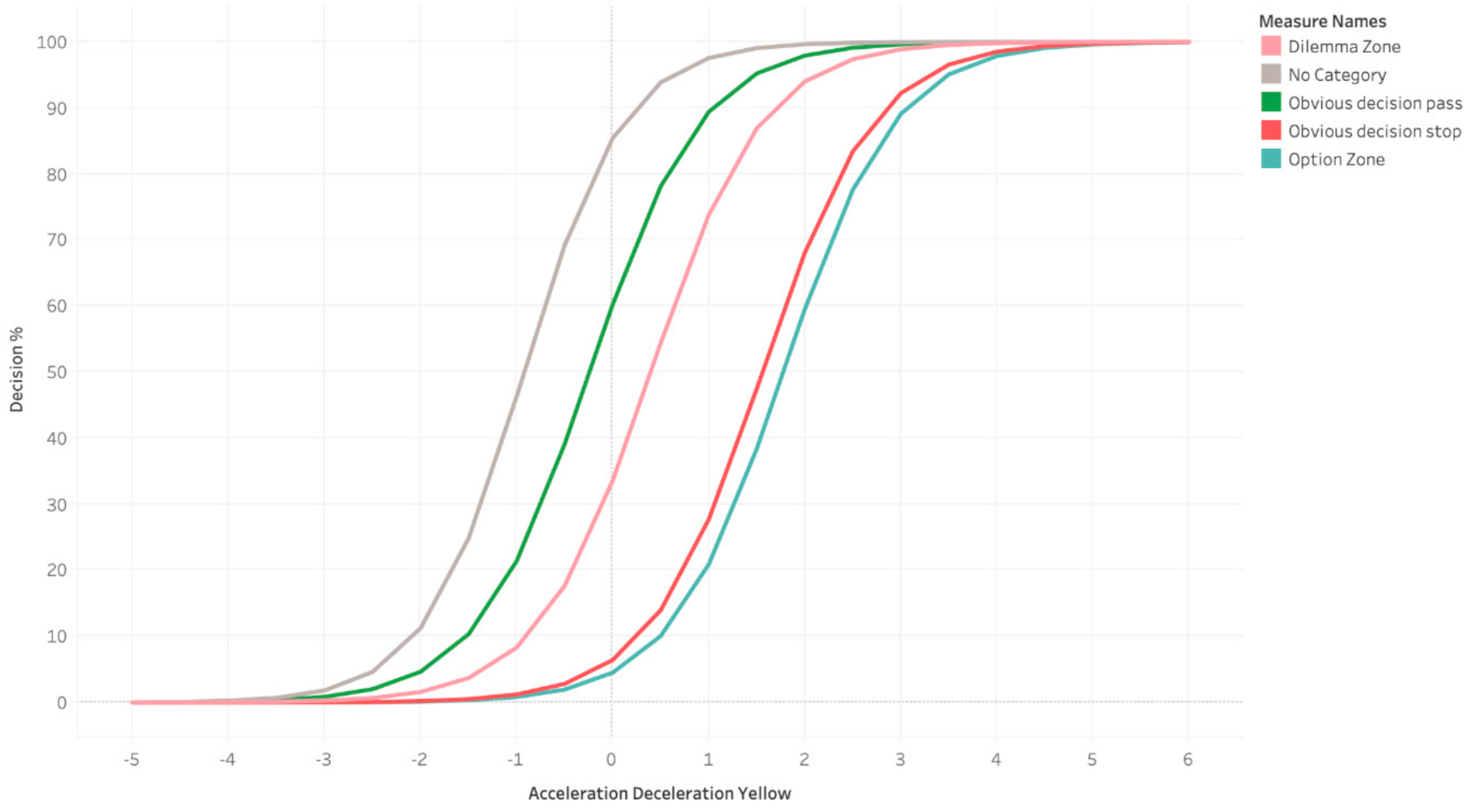
Furthermore, probability charts for the final binary choice model, were also constructed. These charts show that the choice of drivers is influenced by the magnitude of the acceleration/deceleration rate and by the relative position of the vehicles when facing the yellow signal. Aggressive drivers caught in dilemma zone and having acceleration/deceleration rates above −0.50 m/s² are almost 60% more likely to cross the intersection. The corresponding acceleration/deceleration value for conservative drivers is over 0.50 m/s2. For all relevant positions that drivers can be found when they face the yellow signal, the acceleration/deceleration value that increases the chance of drivers crossing the intersection is relatively lower for aggressive drivers than for conservative ones. This practically means that aggressive drivers are more willing to cross the intersection even if they are decelerating on the start of the yellow phase, in contrast to the more conservative drivers for whom the probability of passing is associated with higher acceleration values.

In the following Figure 8 and Figure 9, the “No category” curve represents the probability chart for the initial binary regression model. Comparing one probability curve with the four new curves affected by the relative position of vehicles, it can be observed that the final model can better capture the influence of acceleration/deceleration on drivers’ stop/go decision, not only based on their distance to the stop line but also on their relative position. It is possible to model to a greater extent the influence of acceleration/deceleration on drivers caught in a dilemma zone, whose behavior is a research field of great interest for this and other similar studies.

The calculation of the odds ratio for aggressive to non-aggressive drivers for each relative position is presented in the

Table 10. Odds ratio for aggressive and non-aggressive drivers based on the relative position of vehicles.

	Obvious Decision Pass	Obvious Decision Stop	Option Zone	Dilemma Zone
Odds Ratio	36.93	1.68	1.16	12.29

. Based on the odds ratio, aggressive drivers compared to non-aggressive drivers are almost 37 times more likely to pass the intersection when they face the yellow signal on the obvious decision pass zone, 1.68 times more likely for the obvious decision stop zone, 1.6 times more likely for the option zone and 12.29 times more likely for the dilemma zone.

6. Discussion–Conclusions

In this research effort, two binary logit expressions were built, modeling the drivers’ decision to stop or cross a signalized intersection when facing the yellow indication. The first one is a typical choice model using as explanatory factors only observable and measured data, namely, approaching speed, acceleration/deceleration rate and distance to stop line at the onset of yellow indication.

The second expression attempts to model drivers’ decision by not only using the previous factors but also the aggressiveness level that is associated with each driver. Furthermore, a second additional factor used is the classification of a driver/vehicle in one of four distinct groups according to the so-called relative position of each vehicle in conjunction with the approaching speed.

The first factor of driver aggressiveness can be obtained using the collected data and more specifically the acceleration/deceleration values of observed drivers/vehicles when approaching signalized intersections and facing a traffic light yellow signal in conjunction with initial approaching speed. To do so, the Latent Class Analysis approach was used. Acceleration/deceleration rate values and approaching speed values are grouped in four and three classes, respectively. The LCA analysis performed returned a 45% and 55% probability for aggressive drivers to approach the intersection with high and very high speed, respectively, while a 40% and 60% probability for non-aggressive drivers to approach the intersection with low and medium speed, respectively. Along the same lines, a 50% and 47% chance of approaching the intersection with medium deceleration/acceleration and high acceleration rate, respectively, was returned for the aggressive drivers, while a 71% and 26% chance of approaching the intersection with medium deceleration/acceleration and high acceleration rate, respectively, was returned for the non-aggressive drivers.

The second factor related to the relative position is the group in which a driver/vehicle belongs is achieved by comparing the SSD and CCD with the actual distance of the vehicle from stop line. Depending on the outcome of this comparison, a driver/vehicle may fall in one of four cases as follows: (a) obvious decision to pass, (b) obvious decision to stop, (c) being in option zone, (d) being in dilemma zone.

To include aggressiveness as an additional factor in a binary choice model for stop or go at a signalized intersection would provide a more comprehensive understanding of the driving behavior in such circumstances. The probabilistic power of the first model is considered quite good (91.40%, Nagelkerke R Square 0.83), but driver’s aggressiveness is hidden within the other variables used. Identifying the factor of aggressiveness and separating it from the other factors will help better understand the decision-making mechanism of a driver facing the yellow indication.

The performance of the second model is not better than the first one, but it can provide better explanatory power with respect to driver aggressiveness. Figure 8 and Figure 9 are indicative of the driving behavior differences among aggressive and non-aggressive drivers. The respective figures that represent the distribution of driver’s decision probability are also indicative of the different driver behaviors. Though these specific figures reflect the population of the area under study, the approach adopted can be followed in other areas or countries for both explanatory and confirmatory purposes.

Being able to identify percentages of aggressive drivers enables the calculation of the probability that drivers will cross the intersection even if caught in a dilemma zone or in a zone in which the obvious decision is to stop. Such findings can be valuable when designing a signalized intersection and the signal timing settings, as well as the posted speed limit.

A point worth mentioning is that the approach employed was possible to follow because of the accurate and precise data collected using the UAV technology and the “Tracker Video Analysis and Modeling Tool.” What really matters is the accuracy with which time synchronization of vehicle movement, driver reaction and relative position of the vehicle can be achieved.

Further improvements of the explanatory power of the binary choice models would be possible in the case additional data for other crucial factors become available. Such factors include driver’s gender and age class, which have been found to be closely related to driver aggressiveness. Other factors of importance related to aggressiveness seem to be whether somebody drives alone or not, information that can be obtained by personal observation. Finally, factors such as familiarity with the intersection and the signal timing settings and driving experience may have a strong relation to the driver’s reaction when facing the yellow indication. The latter requires interview surveys to be carried out, which poses a severe obstacle in collecting such information.

Exploring the role of these factors in the overall dilemma zone issue at signalized intersections can be fields of further research. Such research requires additional equipment and resources, which, as in most field studies, are important determinants for both the data collection approach to be selected and their adequacy and precision for the analysis purposes.