
Knotify: An Efficient Parallel Platform for RNA Pseudoknot Prediction Using Syntactic Pattern Recognition

 , , and
Abstract
:1. Introduction
2. Theoretical Background
2.1. RNA
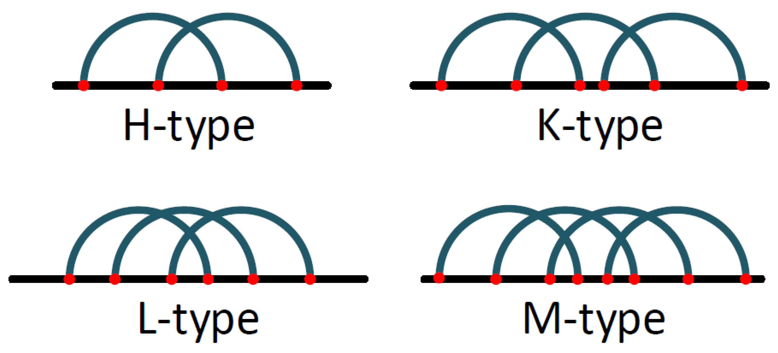
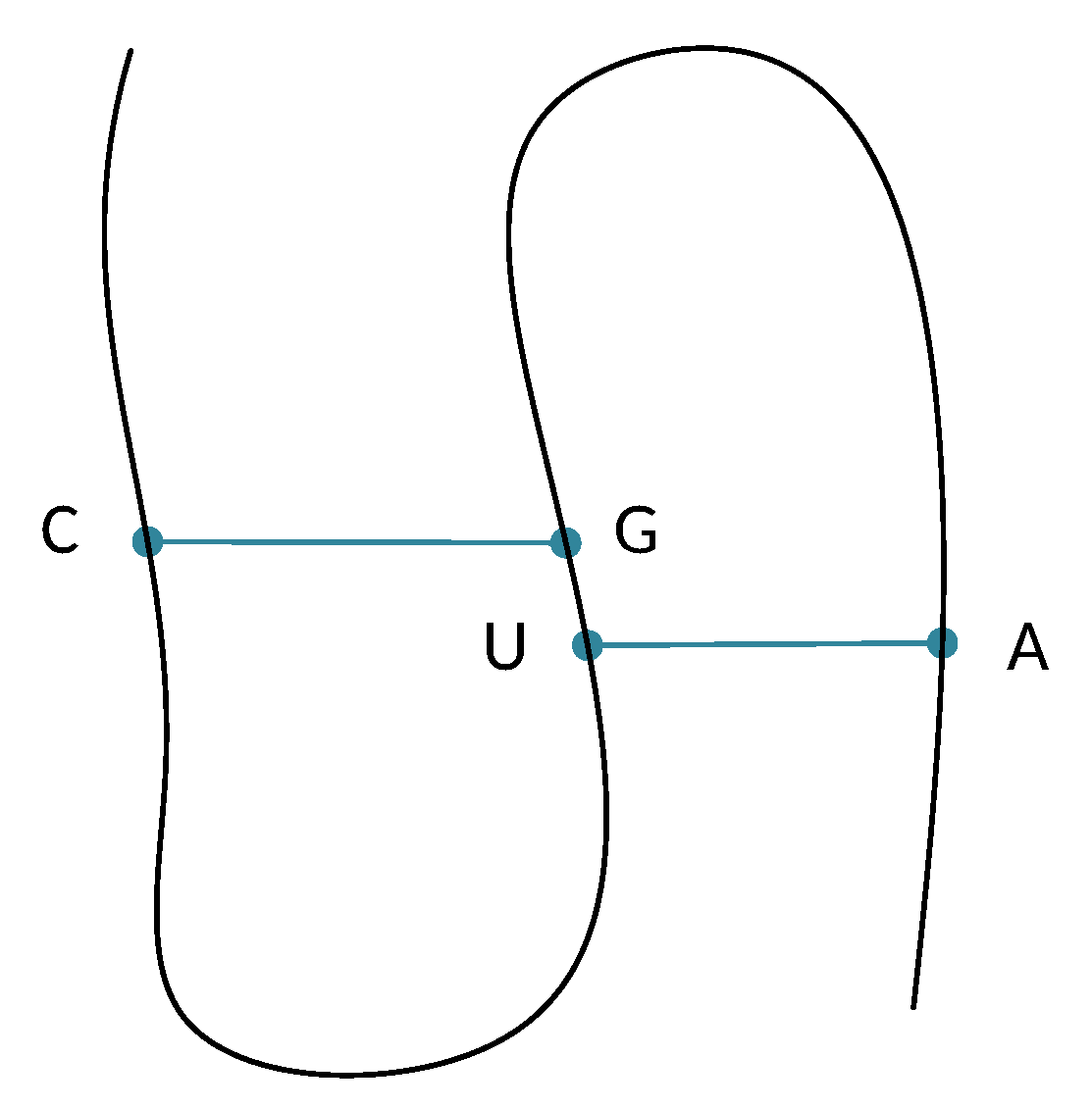
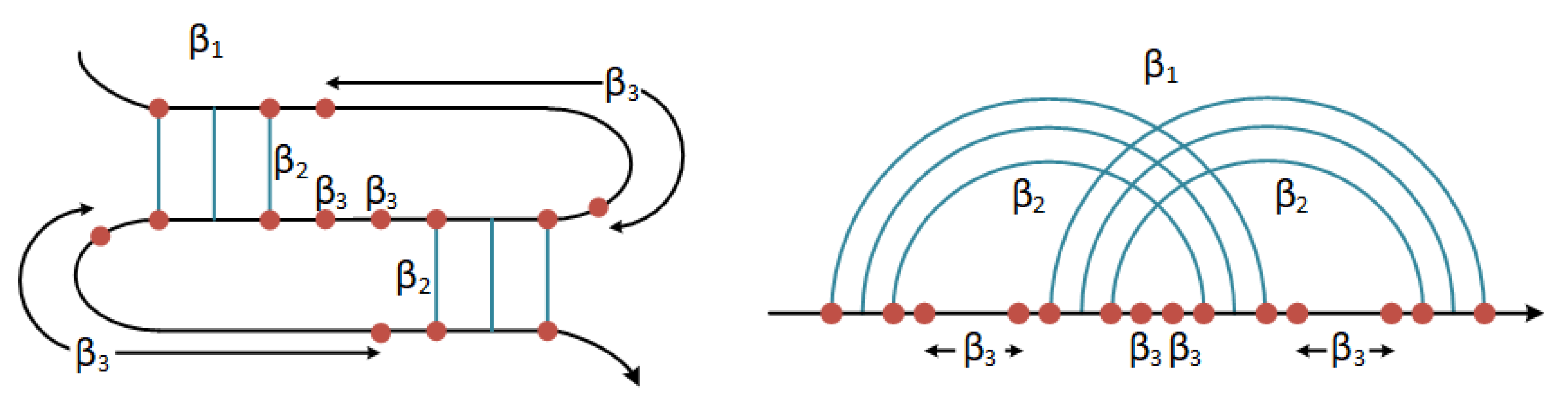
The Pseudoknot Pattern
2.2. Syntactic Pattern Recognition
2.2.1. Context Free Grammars
2.2.2. Primitive Pattern Selection
2.2.3. CFG Parsers
2.2.4. Earley’s Parsing Algorithm
| Algorithm 1 Earley’s Parser Algorithm |
| DECLARE ARRAY_OF_STATES Sets; |
| function INITIALIZE(input_string) |
| n ← LENGTH(input_string) |
| Sets ← CREATE_ARRAY(n + 1) |
| for i ← from 0 to n |
| Sets[i] ← EMPTY_SET |
| endfor |
| function EARLEY_PARSER(input_string, grammar) |
| INITIALIZE(input_string) |
| n ← LENGTH(input_string) |
| ADD_TO_SET((Start → •S, 0), Sets[0]) |
| for i ← from 0 to n |
| for each state in Sets[i] |
| if (state is not completed) |
| if (RIGHT_TO_DOT(state) is a nonterminal) |
| PREDICTOR(state, i, grammar) |
| else |
| SCANNER(state, i, input_string) |
| endif |
| else |
| COMPLETER(state, i) |
| endif |
| endfor |
| endfor |
| return Sets |
| function PREDICTOR((B → α • Cβ, j), i, grammar) |
| for each (C → δ) in GRAMMAR_RULES |
| ADD_STATE_TO_SET((C → •δ, i), Sets[i]) |
| endfor |
| function SCANNER((B → γ• a δ, j), i, input_string) |
| if (a is input_string[i]) |
| ADD_STATE_TO_SET((B → γ a • δ, j), Sets[i+1]) |
| endif |
| function COMPLETER((A → δ•, x), i) |
| for each (B (→ γ• A β), j) in Sets[x] |
| ADD_STATE_TO_SET((B → γ A • β, j), Sets[i]) |
| endfor |
3. Related Work
4. Overview of Our Approach—An Illustrative Example
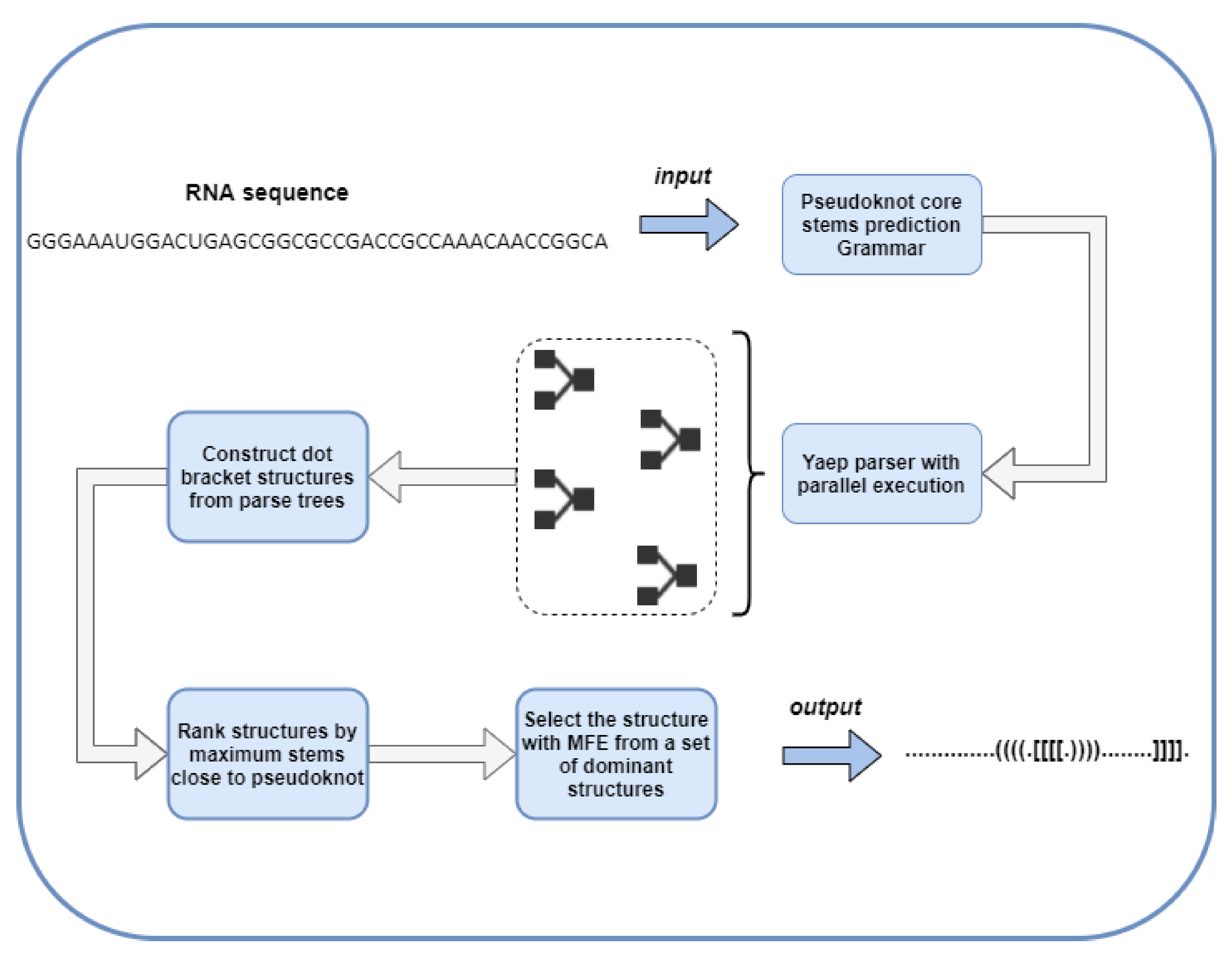
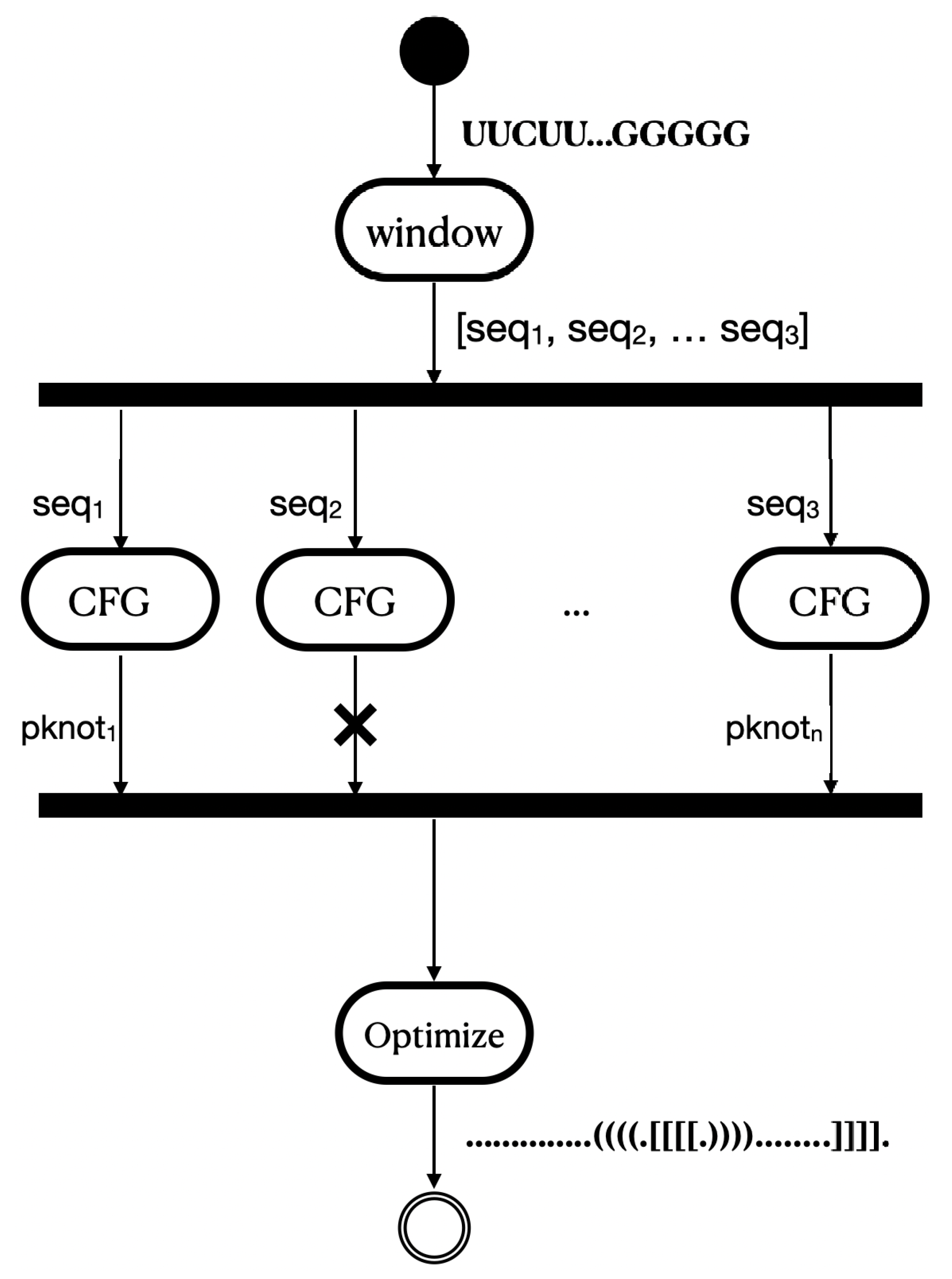
4.1. The Proposed Methodology
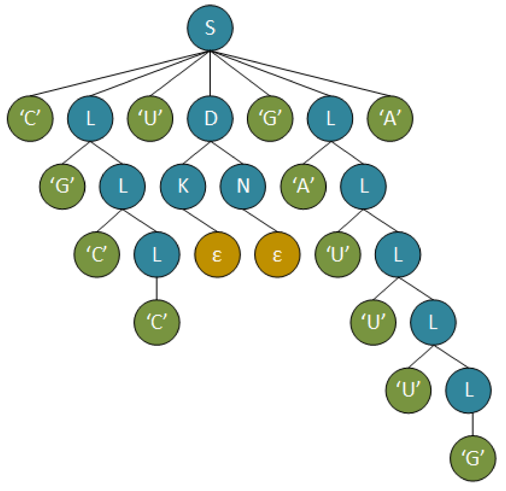
4.1.1. CFG to Identify Pseudoknots
4.1.2. Decorate Core Stems
4.1.3. Optimal Tree Selection
4.1.4. Minimum-Free-Energy Calculation
5. Materials and Methods
Implementation Details
6. Performance Evaluation
6.1. Dataset Presentation
6.2. Methods of Evaluation
6.2.1. Predicting Pseudoknot location
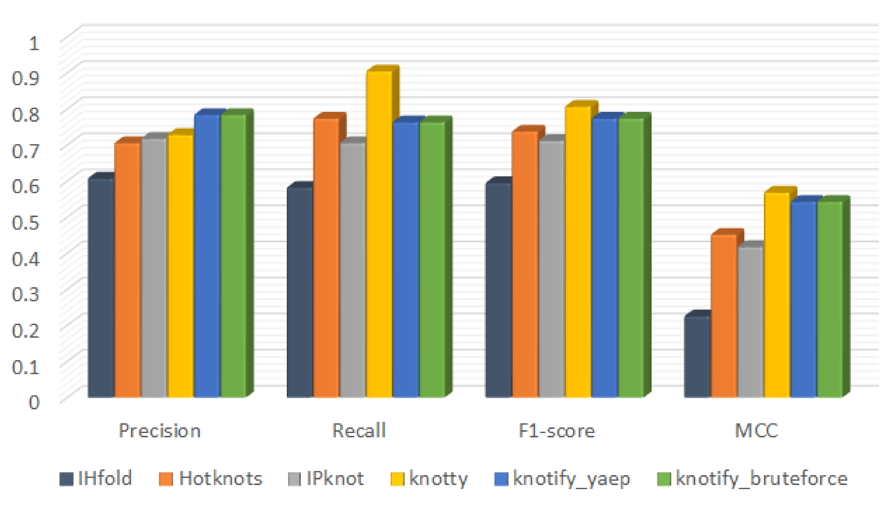
6.2.2. Confusion Matrix
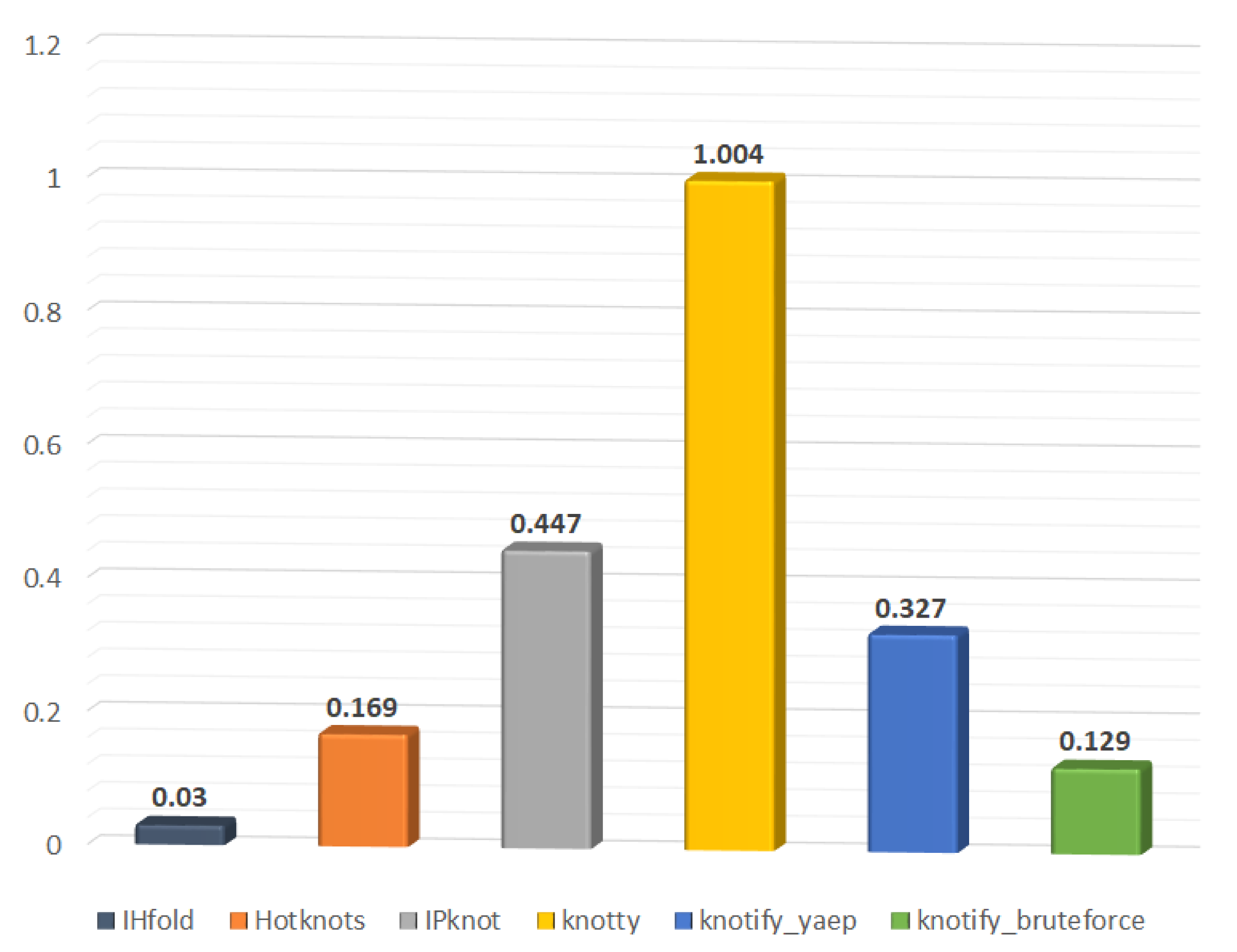
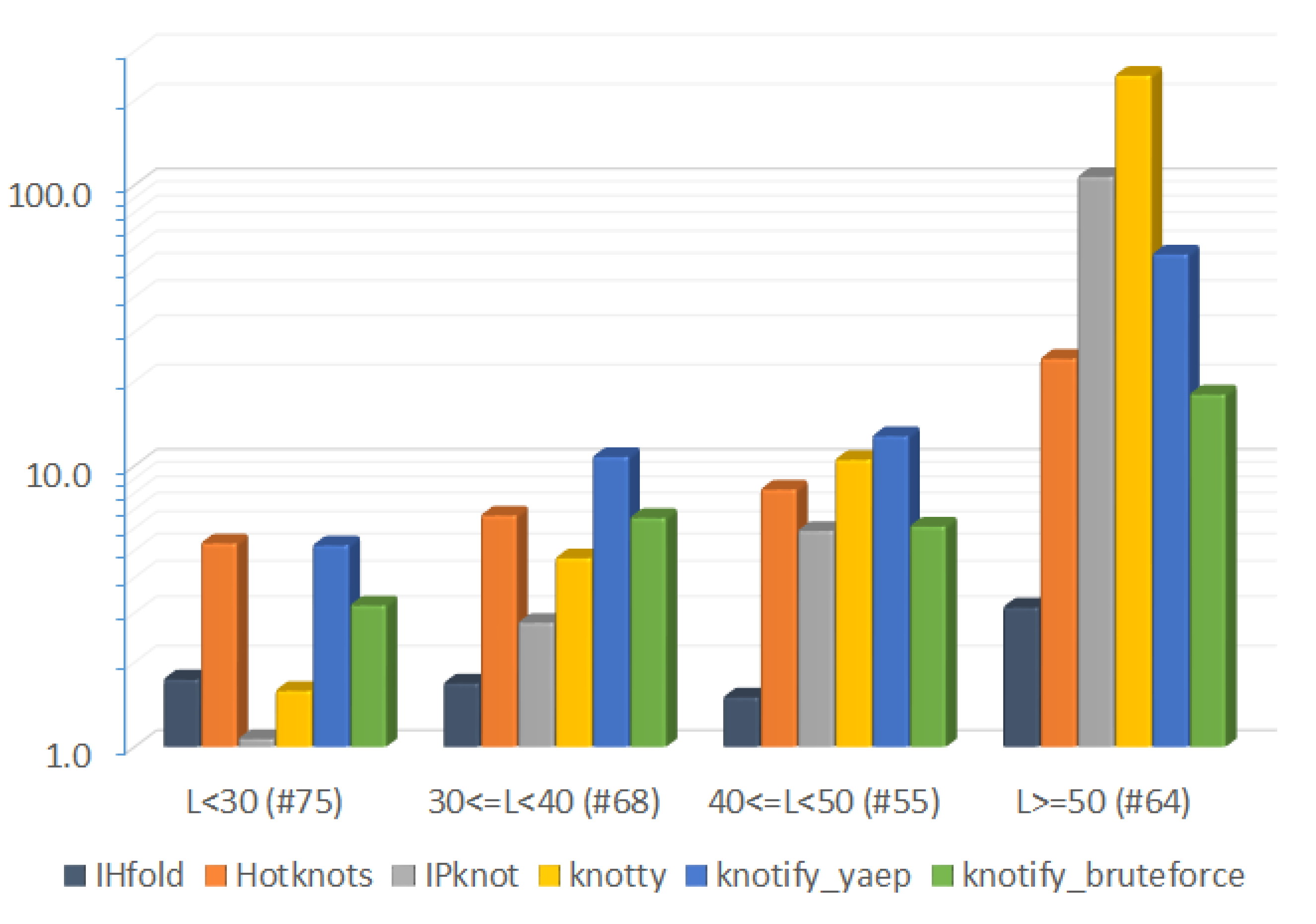
6.2.3. Execution-Time Comparison
7. Discussion and Future Work
Author Contributions
Funding
Institutional Review Board Statement
Informed Consent Statement
Data Availability Statement
Conflicts of Interest
Abbreviations
| CFG | Context-free grammar |
| CGDBP | Coarse-grained dot-bracket prediction |
| CPU | Central processing unit |
| CSV | Comma-separated values |
| CUDA | Compute unified device architecture |
| CYK | Cocke–Younger–Kasami |
| DAG | Direct acyclic graph |
| DNA | Deoxyribonucleic acid |
| FGDPP | Fine-grained dot-plot prediction |
| FPGA | Field programmable gate array |
| GPU | Graphics processing unit |
| IBPMP | Improved base-pair maximization principle |
| LSTM | Long short-term memory |
| MCC | Matthews correlation coefficient |
| MFE | Minimum free energy |
| NAPSS | Nuclear-magnetic-resonance-assisted prediction of secondary structure |
| ncRNA | Non-coding ribonucleic acid |
| NMR | Nuclear magnetic resonance |
| RNA | Ribonucleic acid |
| SCFG | Stochastic context-free grammar |
| TGB | Three-groups-of-band |
| YAEP | Yet another early parser |
References
- Available online: https://bit.ly/dataset_pseudobase_knotify (accessed on 3 January 2022).
- Jabbari, H.; Wark, I.; Montemagno, C.; Will, S. Knotty: Efficient and accurate prediction of complex RNA pseudoknot structures. Bioinformatics 2018, 34, 3849–3856. [Google Scholar] [CrossRef] [PubMed]
- Sato, K.; Kato, Y.; Hamada, M.; Akutsu, T.; Asai, K. IPknot: Fast and accurate prediction of RNA secondary structures with pseudoknots using integer programming. Bioinformatics 2011, 27, 85–93. [Google Scholar] [CrossRef] [PubMed] [Green Version]
- Cech, T.; Steitz, J. The Noncoding RNA Revolution—Trashing Old Rules to Forge New Ones. Cell 2014, 157, 77–94. [Google Scholar] [CrossRef] [PubMed] [Green Version]
- Wu, L.; Belasco, J. Let Me Count the Ways: Mechanisms of Gene Regulation by miRNAs and siRNAs. Mol. Cell 2008, 29, 1–7. [Google Scholar] [CrossRef] [PubMed]
- Doudna, J.; Cech, T. The chemical repertoire of natural ribozymes. Nature 2002, 418, 222–228. [Google Scholar] [CrossRef]
- Ozsolak, F.; Milos, P. RNA sequencing: Advances, challenges and opportunities. Nat. Rev. 2011, 12, 87–98. [Google Scholar] [CrossRef]
- Gawad, C.; Koh, W.; Quake, S. Single-cell genome sequencing: Current state of the science. Nat. Rev. Genet. 2016, 17, 175–188. [Google Scholar] [CrossRef]
- Watson, J.; Crick, F. Molecular Structure Of Nucleic Acids. Am. J. Psychiatry 2003, 160, 623–624. [Google Scholar] [CrossRef]
- Eddy, S. Non-coding RNA genes and the modern RNA world. Nat. Rev. Genet. 2002, 2, 919–929. [Google Scholar] [CrossRef]
- Zuker, M. Calculating Nucleic Acid Secondary Structure. Curr. Opin. Struct. Biol. 2000, 10, 303–310. [Google Scholar] [CrossRef]
- Ritz, J.; Martin, J.; Laederach, A. Evolutionary Evidence for Alternative Structure in RNA Sequence Co-variation. PLoS Comput. Biol. 2013, 9, e1003152. [Google Scholar] [CrossRef] [PubMed] [Green Version]
- Hecker, N.; Seemann, S.; Silahtaroglu, A.; Ruzzo, W.; Gorodkin, J. Associating transcription factors and conserved RNA structures with gene regulation in the human brain. Sci. Rep. 2017, 7, 5756. [Google Scholar] [CrossRef] [Green Version]
- Kubota, M.; Tran, C.; Spitale, R. Progress and challenges for chemical probing of RNA structure inside living cells. Nat. Chem. Biol. 2015, 11, 933–941. [Google Scholar] [CrossRef] [PubMed]
- Spitale, R.; Crisalli, P.; Flynn, R.; Torre, E.; Kool, E.; Chang, H. RNA shape analysis in living cells. Nat. Chem. Biol. 2012, 9, 18–20. [Google Scholar] [CrossRef] [PubMed] [Green Version]
- Chan, D.; Feng, C.; Spitale, R. Measuring RNA structure transcriptome-wide with icSHAPE. Methods 2017, 120, 85–90. [Google Scholar] [CrossRef]
- Shi, Y. A Glimpse of Structural Biology through X-Ray Crystallography. Cell 2014, 159, 995–1014. [Google Scholar] [CrossRef] [Green Version]
- Rietveld, K.; Van Poelgeest, R.; Pleij, C.W.; Van Boom, J.; Bosch, L. The tRNA-Uke structure at the 3′ terminus of turnip yellow mosaic virus RNA. Differences and similarities with canonical tRNA. Nucleic Acids Res. 1982, 10, 1929–1946. [Google Scholar] [CrossRef]
- Kucharík, M.; Hofacker, I.L.; Stadler, P.F.; Qin, J. Pseudoknots in RNA folding landscapes. Bioinformatics 2016, 32, 187–194. [Google Scholar] [CrossRef]
- Staple, D.W.; Butcher, S.E. Pseudoknots: RNA structures with diverse functions. PLoS Biol. 2005, 3, e213. [Google Scholar] [CrossRef] [Green Version]
- Rastogi, T.; Beattie, T.L.; Olive, J.E.; Collins, R.A. A long-range pseudoknot is required for activity of the Neurospora VS ribozyme. EMBO J. 1996, 15, 2820–2825. [Google Scholar] [CrossRef]
- Ke, A.; Zhou, K.; Ding, F.; Cate, J.H.; Doudna, J.A. A conformational switch controls hepatitis delta virus ribozyme catalysis. Nature 2004, 429, 201–205. [Google Scholar] [CrossRef] [PubMed]
- Adams, P.L.; Stahley, M.R.; Kosek, A.B.; Wang, J.; Strobel, S.A. Crystal structure of a self-splicing group I intron with both exons. Nature 2004, 430, 45–50. [Google Scholar] [CrossRef] [PubMed]
- Theimer, C.A.; Blois, C.A.; Feigon, J. Structure of the human telomerase RNA pseudoknot reveals conserved tertiary interactions essential for function. Mol. Cell 2005, 17, 671–682. [Google Scholar] [CrossRef] [PubMed]
- Shen, L.X.; Tinoco, I., Jr. The structure of an RNA pseudoknot that causes efficient frameshifting in mouse mammary tumor virus. J. Mol. Biol. 1995, 247, 963–978. [Google Scholar] [CrossRef]
- Nixon, P.L.; Rangan, A.; Kim, Y.G.; Rich, A.; Hoffman, D.W.; Hennig, M.; Giedroc, D.P. Solution structure of a luteoviral P1–P2 frameshifting mRNA pseudoknot. J. Mol. Biol. 2002, 322, 621–633. [Google Scholar] [CrossRef]
- Michiels, P.J.; Versleijen, A.A.; Verlaan, P.W.; Pleij, C.W.; Hilbers, C.W.; Heus, H.A. Solution structure of the pseudoknot of SRV-1 RNA, involved in ribosomal frameshifting. J. Mol. Biol. 2001, 310, 1109–1123. [Google Scholar] [CrossRef]
- Hopcroft, J.E.; Ullman, J.D. Formal Languages and Their Relation to Automata; Addison-Wesley Longman Publishing Co., Inc.: Boston, MA, USA, 1969. [Google Scholar]
- Chomsky, N. Three models for the description of language. IRE Trans. Inf. Theory 1956, 2, 113–124. [Google Scholar] [CrossRef] [Green Version]
- Sipser, M. Introduction to the Theory of Computation; Thomson Course Technology: Boston, MA, USA, 2006; Volume 2. [Google Scholar]
- Aho, A.V.; Lam, M.S.; Sethi, R.; Ullman, J.D. Compilers: Principles, Techniques, and Tools, 2nd ed.; Addison Wesley: London, UK, 2006. [Google Scholar]
- Younger, D.H. Recognition and parsing of context-free languages in n3. Inf. Control. 1967, 10, 189–208. [Google Scholar] [CrossRef] [Green Version]
- Earley, J. An efficient context-free parsing algorithm. Commun. ACM 1970, 13, 94–102. [Google Scholar] [CrossRef]
- Graham, S.L.; Harrison, M.A.; Ruzzo, W.L. An improved context-free recognizer. ACM Trans. Program. Lang. Syst. 1980, 2, 415–462. [Google Scholar] [CrossRef]
- Ruzzo, W.L. General Context-Free Language Recognition. Ph.D. Thesis, University of California, Berkeley, CA, USA, 1978. [Google Scholar]
- Geng, T.; Xu, F.; Mei, H.; Meng, W.; Chen, Z.; Lai, C. A practical GLR parser generator for software reverse engineering. JNW 2014, 9, 769–776. [Google Scholar] [CrossRef]
- Pavlatos, C.; Dimopoulos, A.C.; Koulouris, A.; Andronikos, T.; Panagopoulos, I.; Papakonstantinou, G. Efficient reconfigurable embedded parsers. Comput. Lang. Syst. Struct. 2009, 35, 196–215. [Google Scholar] [CrossRef]
- Chiang, Y.; Fu, K. Parallel parsing algorithms and VLSI implementations for syntactic pattern recognition. IEEE Trans. Pattern Anal. Mach. Intell. 1984, 6, 302–314. [Google Scholar] [CrossRef] [PubMed]
- Available online: https://github.com/vnmakarov/yaep (accessed on 25 March 2020).
- Antczak, M.; Popenda, M.; Zok, T.; Zurkowski, M.; Adamiak, R.W.; Szachniuk, M. New algorithms to represent complex pseudoknotted RNA structures in dot-bracket notation. Bioinformatics 2018, 34, 1304–1312. [Google Scholar] [CrossRef] [Green Version]
- Lorenz, R.; Bernhart, S.; Höner zu Siederdissen, C.; Tafer, H.; Flamm, C.; Stadler, P.; Hofacker, I. ViennaRNA package 2.0. Algorithms Mol. Biol. 2011, 6, 26. [Google Scholar] [CrossRef]
- Zuker, M. Mfold Web Server for Nucleic Acid Folding and Hybridization Prediction. Nucleic Acids Res. 2003, 31, 3406–3415. [Google Scholar] [CrossRef]
- Bernhart, S.; Hofacker, I.; Will, S.; Gruber, A.; Stadler, P. RNAalifold: Improved Consensus Structure Prediction for RNA Alignments. BMC Bioinform. 2008, 9, 1–13. [Google Scholar] [CrossRef] [Green Version]
- Akutsu, T. Dynamic programming algorithms for RNA secondary structure prediction with pseudoknots. Discret. Appl. Math. 2000, 104, 45–62. [Google Scholar] [CrossRef] [Green Version]
- Lyngsø, R.B.; Pedersen, C.N. RNA pseudoknot prediction in energy-based models. J. Comput. Biol. 2000, 7, 409–427. [Google Scholar] [CrossRef]
- Liu, B.; Mathews, D.H.; Turner, D.H. RNA pseudoknots: Folding and finding. F1000 Biol. Rep. 2010, 2, 8. [Google Scholar] [CrossRef]
- Van Batenburg, F.; Gultyaev, A.P.; Pleij, C.W. An APL-programmed genetic algorithm for the prediction of RNA secondary structure. J. Theor. Biol. 1995, 174, 269–280. [Google Scholar] [CrossRef] [PubMed]
- Isambert, H.; Siggia, E.D. Modeling RNA folding paths with pseudoknots: Application to hepatitis delta virus ribozyme. Proc. Natl. Acad. Sci. USA 2000, 97, 6515–6520. [Google Scholar] [CrossRef] [PubMed] [Green Version]
- Meyer, I.M.; Miklós, I. SimulFold: Simultaneously inferring RNA structures including pseudoknots, alignments, and trees using a Bayesian MCMC framework. PLoS Comput. Biol. 2007, 3, 149. [Google Scholar] [CrossRef] [PubMed]
- Dawson, W.K.; Fujiwara, K.; Kawai, G. Prediction of RNA pseudoknots using heuristic modeling with mapping and sequential folding. PLoS ONE 2007, 2, 905. [Google Scholar] [CrossRef] [Green Version]
- Rivas, E.; Eddy, S.R. A dynamic programming algorithm for RNA structure prediction including pseudoknots. J. Mol. Biol. 1999, 285, 2053–2068. [Google Scholar] [CrossRef]
- Dirks, R.; Pierce, N. Introduction A Partition Function Algorithm for Nucleic Acid Secondary Structure Including Pseudoknots. J. Comput. Chem. 2003, 24, 1664–1677. [Google Scholar] [CrossRef] [Green Version]
- Reeder, J.; Giegerich, R. Design, implementation and evaluation of a practical pseudoknot folding algorithm based on thermodynamics. BMC BioInform. 2004, 5, 104. [Google Scholar] [CrossRef] [Green Version]
- Tabaska, J.E.; Cary, R.B.; Gabow, H.N.; Stormo, G.D. An RNA folding method capable of identifying pseudoknots and base triples. Bioinformatics 1998, 14, 691–699. [Google Scholar] [CrossRef] [Green Version]
- Witwer, C.; Hofacker, I.L.; Stadler, P.F. Prediction of consensus RNA secondary structures including pseudoknots. IEEE/ACM Trans. Comput. Biol. Bioinform. 2004, 1, 66–77. [Google Scholar] [CrossRef]
- Ruan, J.; Stormo, G.D.; Zhang, W. An iterated loop matching approach to the prediction of RNA secondary structures with pseudoknots. Bioinformatics 2004, 20, 58–66. [Google Scholar] [CrossRef] [Green Version]
- Ren, J.; Rastegari, B.; Condon, A.; Hoos, H.H. HotKnots: Heuristic prediction of RNA secondary structures including pseudoknots. RNA 2005, 11, 1494–1504. [Google Scholar] [CrossRef] [PubMed] [Green Version]
- Gumna, J.; Zok, T.; Figurski, K.; Pachulska-Wieczorek, K.; Szachniuk, M. RNAthor—fast, accurate normalization, visualization and statistical analysis of RNA probing data resolved by capillary electrophoresis. PLoS ONE 2020, 15, e0239287. [Google Scholar]
- Wirecki, T.K.; Merdas, K.; Bernat, A.; Boniecki, M.J.; Bujnicki, J.; Stefaniak, F. RNAProbe: A web server for normalization and analysis of RNA structure probing data. Nucleic Acids Res. 2020, 48, W292–W299. [Google Scholar] [CrossRef] [PubMed]
- Bellaousov, S.; Mathews, D.H. ProbKnot: Fast prediction of RNA secondary structure including pseudoknots. RNA 2010, 16, 1870–1880. [Google Scholar] [CrossRef] [PubMed] [Green Version]
- Zhang, L.; Zhang, H.; Mathews, D.H.; Huang, L. ThreshKnot: Thresholded ProbKnot for Improved RNA Secondary Structure Prediction. arXiv 2020, arXiv:1912.12796. [Google Scholar]
- Knudsen, B.; Hein, J. RNA secondary structure prediction using stochastic context-free grammars and evolutionary history. Bioinformatics 1999, 15, 446–454. [Google Scholar] [CrossRef] [Green Version]
- Knudsen, B.; Hein, J. Pfold: RNA Secondary Structure Prediction Using Stochastic Context-Free Grammars. Nucleic Acids Res. 2003, 31, 3423–3428. [Google Scholar] [CrossRef] [Green Version]
- Sukosd, Z.; Knudsen, B.; Vaerum, M.; Kjems, J.; Andersen, E.S. Multithreaded comparative RNA secondary structure prediction using stochastic context-free grammars. BMC Bioinform. 2011, 12, 103. [Google Scholar] [CrossRef]
- Pedersen, J.S.; Meyer, I.M.; Forsberg, R.; Simmonds, P.; Hein, J. A comparative method for finding and folding RNA secondary structures within protein-coding regions. Nucleic Acids Res. 2004, 32, 4925–4936. [Google Scholar] [CrossRef] [Green Version]
- Do, C.B.; Woods, D.A.; Batzoglou, S. CONTRAfold: RNA secondary structure prediction without physics-based models. Bioinformatics 2006, 22, e90–e98. [Google Scholar] [CrossRef]
- Pedersen, J.S.; Bejerano, G.; Siepel, A.; Rosenbloom, K.; Lindblad-Toh, K.; Lander, E.S.; Kent, J.; Miller, W.; Haussler, D. Identification and classification of conserved RNA secondary structures in the human genome. PLoS Comput. Biol. 2006, 2, e33. [Google Scholar] [CrossRef] [PubMed]
- Nawrocki, E.P.; Kolbe, D.L.; Eddy, S.R. Infernal 1.0: Inference of RNA alignments. Bioinformatics 2009, 25, 1335–1337. [Google Scholar] [CrossRef] [PubMed] [Green Version]
- Anderson, J.W.; Haas, P.A.; Mathieson, L.A.; Volynkin, V.; Lyngsø, R.; Tataru, P.; Hein, J. Oxfold: Kinetic folding of RNA using stochastic context-free grammars and evolutionary information. Bioinformatics 2013, 29, 704–710. [Google Scholar] [CrossRef] [PubMed] [Green Version]
- Bradley, R.K.; Pachter, L.; Holmes, I. Specific alignment of structured RNA: Stochastic grammars and sequence annealing. Bioinformatics 2008, 24, 2677–2683. [Google Scholar] [CrossRef] [Green Version]
- Lowe, T.M.; Eddy, S.R. tRNAscan-SE: A program for improved detection of transfer RNA genes in genomic sequence. Nucleic Acids Res. 1997, 25, 955–964. [Google Scholar] [CrossRef]
- Klosterman, P.S.; Uzilov, A.V.; Bendana, Y.R.; Bradley, R.K.; Chao, S.; Kosiol, C.; Goldman, N.; Holmes, I. XRate: A fast prototyping, training and annotation tool for phylo-grammars. BMC Bioinform. 2006, 7, 428. [Google Scholar] [CrossRef] [Green Version]
- Xia, F.; Dou, Y.; Zhou, D.; Li, X. Fine-grained parallel RNA secondary structure prediction using SCFGs on FPGA. Parallel Comput. 2010, 36, 516–530. [Google Scholar] [CrossRef]
- Chang, D.J.; Kimmer, C.; Ouyang, M. Accelerating the nussinov RNA folding algorithm with CUDA/GPU. In Proceedings of the Signal Processing and Information Technology (ISSPIT), Luxor, Egypt, 15–18 December 2010; pp. 120–125. [Google Scholar]
- Available online: https://docs.nvidia.com/cuda/cuda-c-programming-guide/index.html (accessed on 29 January 2022).
- Nussinov, R.; Pieczenik, G.; Griggs, J.R.; Kleitman, D.J. Algorithms for loop matchings. SIAM J. Appl. Math. 1978, 35, 68–82. [Google Scholar] [CrossRef]
- Singh, J.; Hanson, J.; Paliwal, K.; Zhou, Y. RNA secondary structure prediction using an ensemble of two-dimensional deep neural networks and transfer learning. Nat. Commun. 2019, 10, 1–13. [Google Scholar] [CrossRef] [Green Version]
- Wang, L.; Liu, Y.; Zhong, X.; Liu, H.; Lu, C.; Li, C.; Zhang, H. DMfold: A Novel Method to Predict RNA Secondary Structure With Pseudoknots Based on Deep Learning and Improved Base Pair Maximization Principle. Front. Genet. 2019, 10, 143. [Google Scholar] [CrossRef]
- Kangkun, M.; Jun, W.; Yi, X. Prediction of RNA secondary structure with pseudoknots using coupled deep neural networks. Biophys. Rep. 2020, 6, 146–154. [Google Scholar]
- Wang, Y.; Liu, Y.; Wang, S.; Liu, Z.; Gao, Y.; Zhang, H.; Dong, L. ATTfold: RNA Secondary Structure Prediction With Pseudoknots Based on Attention Mechanism. Front. Genet. 2020, 11, 1564. [Google Scholar] [CrossRef] [PubMed]
- Available online: https://github.com/ntua-dslab/knotify/tree/02-mdpi-2021-r2 (accessed on 29 January 2022).
- Trotta, E. On the normalization of the minimum free energy of RNAs by sequence length. PLoS ONE 2014, 9, e113380. [Google Scholar] [CrossRef] [PubMed] [Green Version]
- Nussinov, R.; Jacobson, A.B. Fast algorithm for predicting the secondary structure of single-stranded RNA. Proc. Natl. Acad. Sci. USA 1980, 77, 6309–6313. [Google Scholar] [CrossRef] [Green Version]
- Mathews, D.H. Using an RNA secondary structure partition function to determine confidence in base pairs predicted by free energy minimization. RNA 2004, 10, 1178–1190. [Google Scholar] [CrossRef] [Green Version]
- Rivas, E.; Eddy, S.R. Noncoding RNA gene detection using comparative sequence analysis. BMC Bioinform. 2001, 2, 8. [Google Scholar] [CrossRef] [Green Version]
- Chu, Y.; Corey, D.R. RNA Sequencing: Platform Selection, Experimental Design, and Data Interpretation. Nucleic Acid Ther. 2012, 22, 271–274. [Google Scholar] [CrossRef]
- Mathews, D.; Sabina, J.; Zuker, M.; Turner, D. Expanded sequence dependence of thermodynamic parameters improves prediction of RNA secondary structure1. J. Mol. Biol. 1999, 288, 911–940. [Google Scholar] [CrossRef] [Green Version]
- McKinney, W. Pandas: A foundational Python library for data analysis and statistics. Python High Perform. Sci. Comput. 2011, 14, 1–9. [Google Scholar]
- Jabbari, H.; Condon, A. A fast and robust iterative algorithm for prediction of RNA pseudoknotted secondary structures. MC Bioinform. 2014, 15, 147. [Google Scholar] [CrossRef] [Green Version]
- Andrikos, C.; Rassias, G.; Tsanakas, P.; Maglogiannis, I. An enhanced device-transparent real-time teleconsultation environment for radiologists. IEEE J. Biomed. Health Inform. 2018, 23, 374–386. [Google Scholar] [CrossRef] [PubMed]
- Andrikos, C.; Rassias, G.; Tsanakas, P.; Maglogiannis, I. Real-time medical collaboration services over the web. In Proceedings of the 2015 37th Annual International Conference of the IEEE Engineering in Medicine and Biology Society (EMBC), Milan, Italy, 25–29 August 2015; pp. 1393–1396. [Google Scholar]


| # | Syntactic Rules |
|---|---|
| 0 | S → “A” L “A” D “U” L “U” |
| 1 | S → “U” L “A” D “A” L “U” |
| 2 | S → “C” L “A” D “G” L “U” |
| 3 | S → “G” L “A” D “C” L “U” |
| 4 | S → “A” L “U” D “U” L “A” |
| 5 | S → “U” L “U” D “A” L “A” |
| 6 | S → “C” L “U” D “G” L “A” |
| 7 | S → “G” L “U” D “C” L “A” |
| 8 | S → “A” L “C” D “U” L “G” |
| 9 | S → “U” L “C” D “A” L “G” |
| 10 | S → “C” L “C” D “G” L “G” |
| 11 | S → “G” L “C” D “C” L “G” |
| 12 | S → “A” L “G” D “U” L “C” |
| 13 | S → “U” L “G” D “A” L “C” |
| 14 | S → “C” L “G” D “G” L “C” |
| 15 | S → “G” L “G” D “C” L “C” |
| 16 | L → “A” L |
| 17 | L → “U” L |
| 18 | L → “C” L |
| 19 | L → “G” L |
| 20 | L → “A” |
| 21 | L → “U” |
| 22 | L → “C” |
| 23 | L → “G” |
| 24 | D → K N |
| 25 | K → “A” |
| 26 | K → “U” |
| 27 | K → “C” |
| 28 | K → “G” |
| 29 | K |
| 30 | N → “A” |
| 31 | N → “u” |
| 32 | N → “C” |
| 33 | N → “G” |
| 34 | N |
| String enumeration | 1 | 2 | 3 | 4 | 5 | 6 | 7 | 8 | 9 | 10 | 11 | 12 | 13 | 14 | 15 | 16 | 17 | 18 | 19 |
| String | C | C | A | U | C | G | C | C | U | G | A | U | U | U | G | A | G | G | A |
| Parser output | . | . | . | . | [ | . | . | . | ( | ] | . | . | . | . | . | ) | . | . | . |
| Step 1 | . | . | . | . | [ | . | . | ( | ( | ] | . | . | . | . | . | ) | ) | . | . |
| Step 2 | . | . | . | . | [ | . | ( | ( | ( | ] | . | . | . | . | . | ) | ) | ) | . |
| Step 3 | . | . | . | [ | [ | . | ( | ( | ( | ] | ] | . | . | . | . | ) | ) | ) | . |
| step 4 | . | . | [ | [ | [ | . | ( | ( | ( | ] | ] | ] | . | . | . | ) | ) | ) | . |
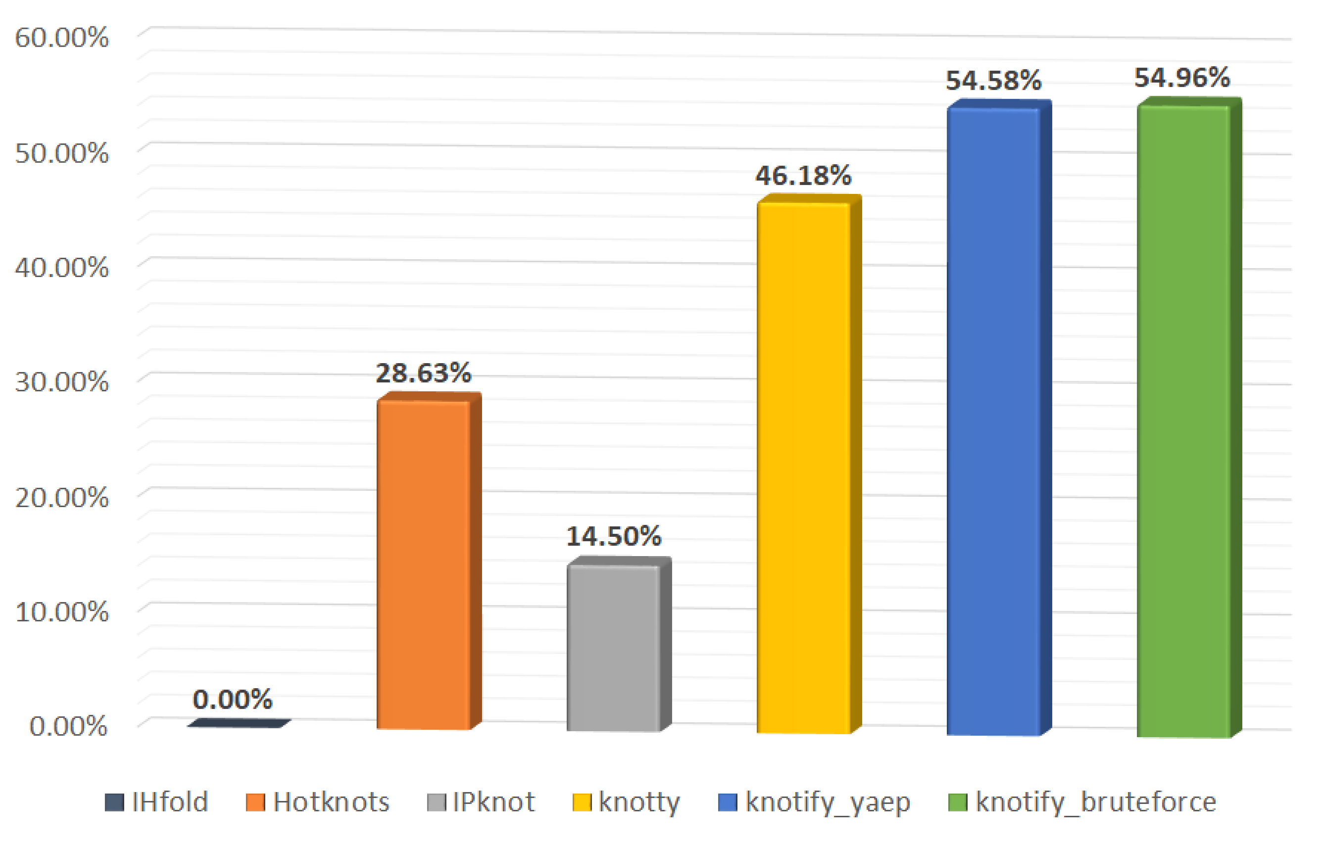
| Platform | Exact Matches | Exact Matches (%) |
|---|---|---|
| IHFold | 0 | 0 |
| HotKnots | 75 | 28.6 |
| IPknot | 38 | 14.5 |
| Knotty | 121 | 46.1 |
| knotify_yaep | 143 | 54.5 |
| knotify_bruteforce | 144 | 54.9 |
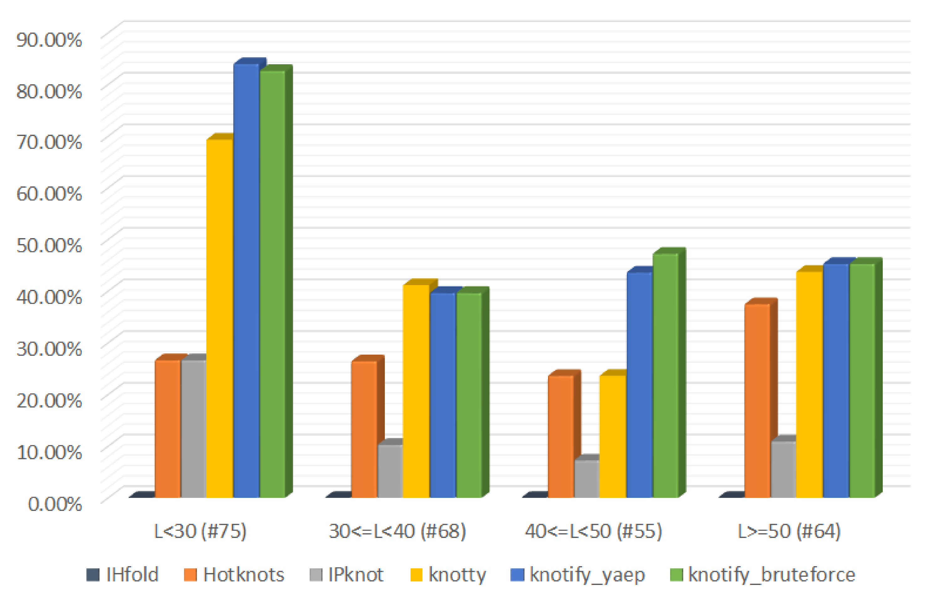
| L < 30 (#75) | 30 <= L < 40 (#68) | 40 <= L < 50 (#55) | L >= 50 (#64) | |||||
|---|---|---|---|---|---|---|---|---|
| Platform | Exact | Exact | Exact | Exact | Exact | Exact | Exact | Exact |
| Matches | Matches (%) | Matches | Matches (%) | Matches | Matches (%) | Matches | Matches (%) | |
| IHFold | 0 | 0.00 | 0 | 0.00 | 0 | 0.00 | 0 | 0.00 |
| Hotknots | 20 | 26.67 | 18 | 26.47 | 13 | 23.64 | 24 | 37.5 |
| IPknot | 20 | 26.67 | 7 | 10.29 | 4 | 7.27 | 7 | 10.94 |
| Knotty | 52 | 69.33 | 28 | 41.18 | 13 | 23.64 | 28 | 43.75 |
| knotify_yaep | 63 | 84.00 | 27 | 39.71 | 24 | 43.64 | 29 | 45.31 |
| knotify_bruteforce | 62 | 82.67 | 27 | 39.71 | 26 | 47.27 | 29 | 45.31 |
| Platform | tp | tn | fp | fn | Precision | Recall | F1-Score | MCC |
|---|---|---|---|---|---|---|---|---|
| IHFold | 3056 | 3556 | 1968 | 2196 | 0.608 | 0.582 | 0.595 | 0.226 |
| Hotknots | 4180 | 3632 | 1744 | 1220 | 0.706 | 0.774 | 0.738 | 0.452 |
| IPknot | 3872 | 3767 | 1522 | 1615 | 0.718 | 0.706 | 0.712 | 0.418 |
| Knotty | 5026 | 3352 | 1870 | 528 | 0.729 | 0.905 | 0.807 | 0.569 |
| knotify_yaep | 4212 | 4102 | 1162 | 1300 | 0.784 | 0.764 | 0.774 | 0.543 |
| knotify_bruteforce | 4214 | 4101 | 1160 | 1301 | 0.784 | 0.764 | 0.774 | 0.543 |
| Platform | tp | tn | fp | fn | Precision | Recall | F1-Score | MCC |
|---|---|---|---|---|---|---|---|---|
| IHFold | 738 | 522 | 118 | 513 | 0.862 | 0.590 | 0.701 | 0.386 |
| Hotknots | 904 | 492 | 156 | 339 | 0.853 | 0.727 | 0.785 | 0.465 |
| IPknot | 916 | 514 | 124 | 337 | 0.881 | 0.731 | 0.799 | 0.510 |
| Knotty | 1196 | 469 | 146 | 80 | 0.891 | 0.937 | 0.914 | 0.722 |
| knotify_yaep | 1244 | 486 | 134 | 27 | 0.903 | 0.979 | 0.939 | 0.805 |
| knotify_bruteforce | 1242 | 485 | 136 | 28 | 0.901 | 0.978 | 0.938 | 0.802 |
| Platform | tp | tn | fp | fn | Precision | Recall | F1-Score | MCC |
|---|---|---|---|---|---|---|---|---|
| IHFold | 550 | 832 | 352 | 587 | 0.610 | 0.484 | 0.539 | 0.191 |
| Hotknots | 922 | 851 | 294 | 254 | 0.758 | 0.784 | 0.771 | 0.528 |
| IPknot | 824 | 823 | 314 | 360 | 0.724 | 0.696 | 0.710 | 0.420 |
| Knotty | 1078 | 802 | 324 | 117 | 0.769 | 0.902 | 0.830 | 0.628 |
| knotify_yaep | 988 | 893 | 296 | 144 | 0.769 | 0.873 | 0.818 | 0.627 |
| knotify_bruteforce | 988 | 893 | 296 | 144 | 0.769 | 0.873 | 0.818 | 0.627 |
| Platform | tp | tn | fp | fn | Precision | Recall | F1-Score | MCC |
|---|---|---|---|---|---|---|---|---|
| IHFold | 612 | 864 | 478 | 418 | 0.561 | 0.594 | 0.577 | 0.237 |
| Hotknots | 792 | 857 | 510 | 213 | 0.608 | 0.788 | 0.687 | 0.412 |
| IPknot | 764 | 911 | 410 | 287 | 0.651 | 0.727 | 0.687 | 0.414 |
| Knotty | 904 | 817 | 524 | 127 | 0.633 | 0.877 | 0.735 | 0.492 |
| knotify_yaep | 764 | 1010 | 298 | 300 | 0.719 | 0.718 | 0.719 | 0.490 |
| knotify_bruteforce | 772 | 1012 | 290 | 298 | 0.727 | 0.721 | 0.724 | 0.499 |
| Platform | tp | tn | fp | fn | Precision | Recall | F1-Score | MCC |
|---|---|---|---|---|---|---|---|---|
| IHFold | 1156 | 1338 | 1020 | 678 | 0.531 | 0.63 | 0.577 | 0.196 |
| Hotknots | 1562 | 1432 | 784 | 414 | 0.666 | 0.790 | 0.723 | 0.439 |
| IPknot | 1368 | 1519 | 674 | 631 | 0.670 | 0.684 | 0.677 | 0.377 |
| Knotty | 1848 | 1264 | 876 | 204 | 0.678 | 0.901 | 0.774 | 0.515 |
| knotify_yaep | 1216 | 1713 | 434 | 829 | 0.737 | 0.595 | 0.658 | 0.402 |
| knotify_bruteforce | 1212 | 1711 | 438 | 831 | 0.735 | 0.593 | 0.656 | 0.398 |
| Platform | Average Time (s) | Total Time (s) |
|---|---|---|
| IHFold | 0.030 | 8.096 |
| Hotknots | 0.169 | 44.432 |
| IPknot | 0.447 | 117.246 |
| Knotty | 1.004 | 263.303 |
| knotify_yaep | 0.327 | 85.756 |
| knotify_bruteforce | 0.129 | 33.894 |
| Platform | Average Time (s) | Total Time (s) |
|---|---|---|
| IHFold | 0.0233 | 1.748 |
| Hotknots | 0.0709 | 5.314 |
| IPknot | 0.0143 | 1.070 |
| Knotty | 0.0212 | 1.590 |
| knotify_yaep | 0.0697 | 5.226 |
| knotify_bruteforce | 0.0427 | 3.204 |
| Platform | Average Time (s) | Total Time (s) |
|---|---|---|
| IHFold | 0.0248 | 1.689 |
| Hotknots | 0.0982 | 6.680 |
| IPknot | 0.0408 | 2.777 |
| Knotty | 0.0692 | 4.703 |
| knotify_yaep | 0.1589 | 10.808 |
| knotify_bruteforce | 0.0964 | 6.555 |
| Platform | Average Time (s) | Total Time (s) |
|---|---|---|
| IHFold | 0.0274 | 1.507 |
| Hotknots | 0.1503 | 8.264 |
| IPknot | 0.107 | 5.886 |
| Knotty | 0.1918 | 10.546 |
| knotify_yaep | 0.2331 | 12.821 |
| knotify_bruteforce | 0.111 | 6.103 |
| Platform | Average Time (s) | Total Time (s) |
|---|---|---|
| IHFold | 0.0492 | 3.151 |
| Hotknots | 0.3777 | 24.172 |
| IPknot | 1.679 | 107.511 |
| Knotty | 3.851 | 246.462 |
| knotify_yaep | 0.8891 | 56.900 |
| knotify_bruteforce | 0.2817 | 18.030 |
Publisher’s Note: MDPI stays neutral with regard to jurisdictional claims in published maps and institutional affiliations. |
© 2022 by the authors. Licensee MDPI, Basel, Switzerland. This article is an open access article distributed under the terms and conditions of the Creative Commons Attribution (CC BY) license (https://creativecommons.org/licenses/by/4.0/).
Share and Cite
Andrikos, C.; Makris, E.; Kolaitis, A.; Rassias, G.; Pavlatos, C.; Tsanakas, P. Knotify: An Efficient Parallel Platform for RNA Pseudoknot Prediction Using Syntactic Pattern Recognition. Methods Protoc. 2022, 5, 14. https://0-doi-org.brum.beds.ac.uk/10.3390/mps5010014
Andrikos C, Makris E, Kolaitis A, Rassias G, Pavlatos C, Tsanakas P. Knotify: An Efficient Parallel Platform for RNA Pseudoknot Prediction Using Syntactic Pattern Recognition. Methods and Protocols. 2022; 5(1):14. https://0-doi-org.brum.beds.ac.uk/10.3390/mps5010014
Chicago/Turabian StyleAndrikos, Christos, Evangelos Makris, Angelos Kolaitis, Georgios Rassias, Christos Pavlatos, and Panayiotis Tsanakas. 2022. "Knotify: An Efficient Parallel Platform for RNA Pseudoknot Prediction Using Syntactic Pattern Recognition" Methods and Protocols 5, no. 1: 14. https://0-doi-org.brum.beds.ac.uk/10.3390/mps5010014