
SimpliFI: Hardware Simulation of Embedded Software Fault Attacks


Department of Electrical and Computer Engineering, Worcester Polytechnic Institute, Worcester, MA 01609, USA
*
Author to whom correspondence should be addressed.
Cryptography 2021, 5(2), 15; https://0-doi-org.brum.beds.ac.uk/10.3390/cryptography5020015
Submission received: 8 May 2021
/
Revised: 29 May 2021
/
Accepted: 3 June 2021
/
Published: 7 June 2021
(This article belongs to the Special Issue Feature Papers in Hardware Security)
Abstract
:Fault injection simulation on embedded software is typically captured using a high-level fault model that expresses fault behavior in terms of programmer-observable quantities. These fault models hide the true sensitivity of the underlying processor hardware to fault injection, and they are unable to correctly capture fault effects in the programmer-invisible part of the processor microarchitecture. We present SimpliFI, a simulation methodology to test fault attacks on embedded software using a hardware simulation of the processor running the software. We explain the purpose and advantage of SimpliFI, describe automation of the simulation framework, and apply SimpliFI on a BRISC-V embedded processor running an AES application.
1. Introduction
Fault attacks are a hardware-oriented attack on the system-level security of hardware or software. Fault attacks use precisely tuned fault injection on those systems to induce privilege escalation or to cause information leakage. Defense against fault attacks is not easy, because the designer must understand the mechanism of fault injection and fault propagation for every available fault injection point, and resolve which of the faults may induce loss of data or control. The attacker’s job is easier, since a successful fault attack is typically any fault injection that leads to the intended privilege escalation or information leakage. Moreover, to perform a fault attack, the attacker does not have to understand the exact nature of the fault.
To develop a countermeasure against a fault attack, the fault attack vector must be precisely understood. The traditional defense against a fault attack is therefore to over-design the system through temporal and spatial redundancy in the design. This is expensive and only applicable to designs where performance and/or cost is secondary to security. To design more efficient countermeasures, it is necessary in the first place to understand how faults are injected and propagated.
In this paper, we propose an environment to study fault attacks on software systems. Surprisingly, there is no general methodology to deal with simulation of hardware fault vectors in fault attack simulation on software systems. Typically, software fault attack simulation requires forfeiting physical accuracy in return for more efficient analysis of the fault impact on software data flow and control flow [1]. For example, a designer can choose a high-level fault model such as bit-flip or instruction-skip, and then evaluate the sensitivity of the software system against attacks based on such a fault model [2]. This is a simplification of reality, and there is not guarantee that the physical processor that runs the secure software will exhibit the same fault behavior as the presumed fault model. Therefore, many of the current methodologies to study fault attacks on software systems are based on hardware prototypes [3,4]. The results of such evaluations are highly device dependent, and often the precise nature of the fault still cannot be understood because the hardware prototype is a black box from fault evaluation perspective.
In this paper, we propose a SImulation Methodology for embedded Processors to Learn the Impacts of Fault Injection (SimpliFI), which relies on hardware simulation to obtain physically-accurate software fault evaluation results. This approach uses a low-level model of the physical attributes of an actual device, such as gate layout and signal propagation, to predict realistic responses to fault injection attacks. By encapsulating hardware fault propagation and software execution in one simulation, SimpliFI supports root-cause analysis of software fault impacts for both short instruction sequences and full applications. To our knowledge, SimpliFI is the first design-time methodology that enables automated fault evaluation and explains software-level fault effects through their manifestation in the device.
This article presents SimpliFI as a high-level generic framework for automatic evaluation of embedded software fault vulnerabilities, and presents an implementation of the framework for the open-source BRISC-V embedded processor [5,6]. The results collected by the framework are able to show how different fault injection parameters affect the processor state, which faults propagate to program outputs, and which subsets of the processor microarchitecture are more susceptible to fault injection. This article makes the following contributions to the field. First, we present a simulation methodology of root-cause analysis of fault attacks in software, where we study fault propagation using hardware simulation and fault impact analysis at the instruction-level and program-level in software. Second, we present an automation framework that can exhaustively inject faults in a software application and classify their outcome at instruction-level and program-level. We are able to deduce device-specific microarchitectural effects from the observed fault patterns. Third, we describe our experimental results on a SimpliFI prototype for the BRISC-V processor running AES encryption.
The remainder of this article is structured as follows. Section 2 discusses background topics in fault injection techniques and current fault injection analysis methods. Section 3 presents SimpliFI as a generic framework that defines specific functional requirements. Section 3 also discusses a practical implementation of the framework using the Xilinx Vivado Design Suite to analyze a BRISC-V FPGA core. Section 4 discusses how results from SimpliFI provide insight into instruction-level and application-level fault vulnerabilities of embedded software running on BRISC-V. Finally, Section 5 concludes by discussing SimpliFI’s place in the security electronic design automation tool landscape and proposing useful extensions for future work.
2. Related Work
In this section, we describe the design space of tools to study software fault injection, and we review related work.
2.1. Design Space of Fault Attack Simulation
While fault injection techniques have been used to exploit both digital systems and embedded software [7,8], a physical fault always manifests as a 0 or 1 bit in the hardware state. The fault injection technique always causes a change at the hardware level, but whether or not faulty data will be stored in the registered hardware state is not always predictable. In this paper, we adopt the following definitions.
- Fault Injection/Attack—The act of tampering with the system and parameters and environment to cause faults in the hardware.
- Fault Manifestation—The process by which injected faults affect the circuitry and are either successfully incorporated into the hardware state or otherwise lost.
- Hardware Faults/Faulty Bits— The bits in the hardware state that are successfully affected by an injected fault.
- Hardware Fault Propagation—The process by which faulty bits propagate through the hardware, creating erroneous bits in different parts of the circuitry.
- Software Fault—Bits in the software-level state that have been changed by hardware faults. Not every faulty bit in the hardware will have an impact on the correctness of software execution.
- Software Fault Impact/Response—The general changes in software behavior caused by software faults. This may be described quantitatively or qualitatively in terms of instruction execution.
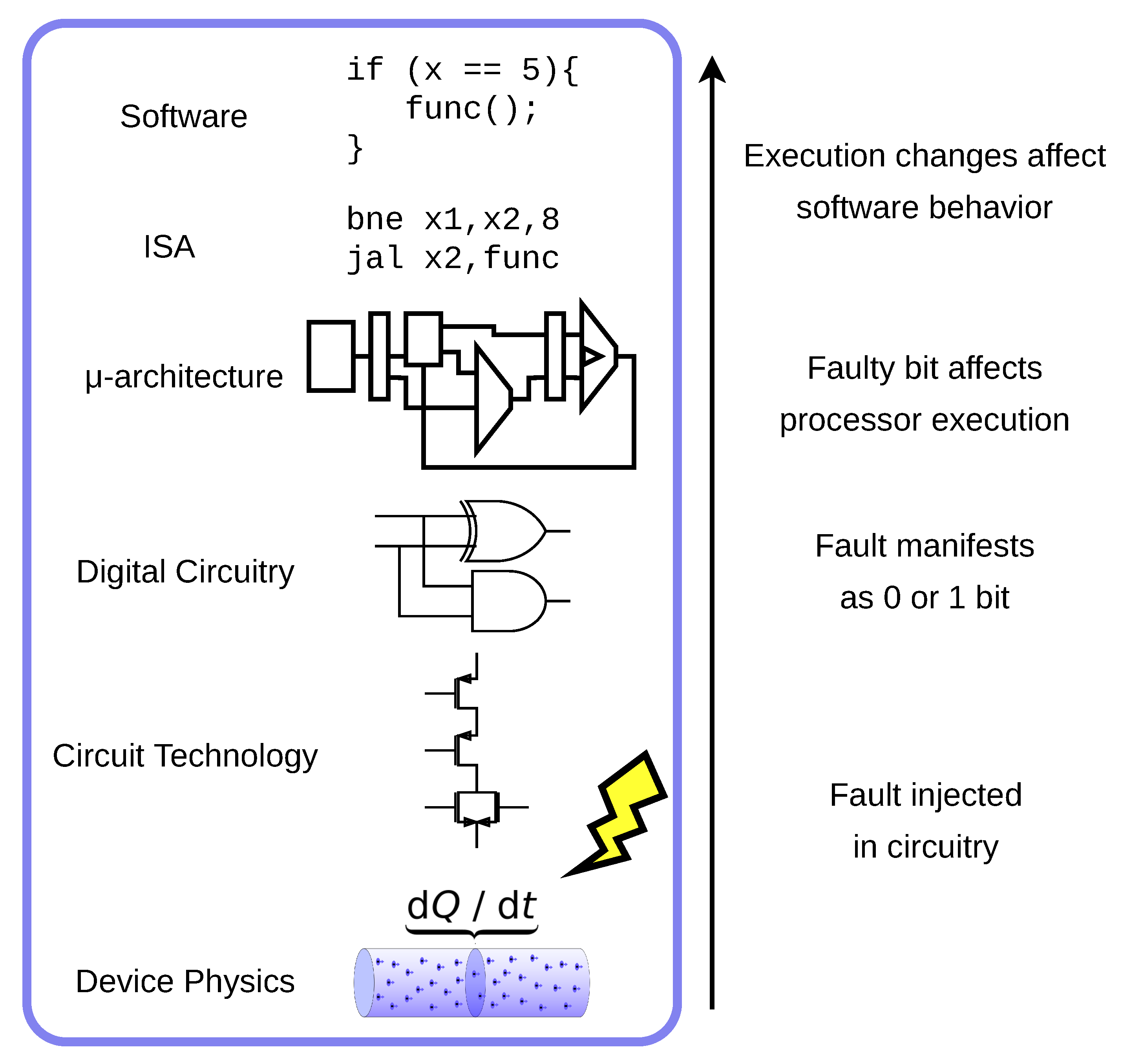
Even when a fault injection successfully induces faulty bits in the hardware state, there is a large abstraction stack that separates the hardware fault from software-level behavior [9]. Figure 1 summarizes the layering of abstractions that a fault travels through, when fault injection is used to attack a software program. Between different ISAs, microarchitectures, and physical implementations, any two given embedded processors may respond differently to the same fault injection attacks. At the hardware level, differences in the physical circuitry and layout can lead to different impacts on the hardware state from the same fault. For example, the program counter in two different physical implementations of the same processor may produce different faulty states for the same clock glitch attack due to differences in the critical paths. At the architecture level, microarchitectural differences of the same ISA can lead to very different fault propagation behavior simply due to the nature of the microarchitecture having unique impacts on data flow.
Due to the many abstraction layers that exist between fault injection and eventual software fault analysis, there are multiple solutions to address fault attack simulation on embedded software. Indeed, even though the physics of fault injection do involve fault manifestation and propagation through the complete hardware and software stack, this is not essential. By selecting an appropriate fault model (e.g. stuck-at-1, instruction-skip) it is possible to abstract the lower layers of the fault injection stack away at the loss of modeling accuracy and the gain of simulation speed.
2.2. Fault Characterization of Embedded Software
In the past decade, multiple studies have focused on characterizing the effects of embedded software fault attacks on various platforms. While the results vary by platform, authors agree that most results can be explained by replacing the original instruction with a different one [10,11,12,13]. Hence, these results confirm empirically what we would expect to determine with SimpliFI in a simulation.
Moro et al. tested EM faults on an ARM Cortex-M3, focusing heavily on applying faults to a single load instruction while fetching it from flash memory [10]. The authors concluded that all faults that are explained by single instruction replacement must be faults on the instruction fetch, and that all unexplained outcomes are faults on the data fetch. These observations culminate in a simple model, where the time of the fault corresponds to the number of 1s that will be read from the memory data line. This result was deemed device dependent because the bus precharge value is responsible for whether a stuck at 0 or stuck at 1 fault manifests.
Proy et al. provided more insight into fault behavior on an ARM Cortex-A9, compared to the single instruction analysis from the prior study [11]. Proy concludes that single faults can be explained in terms of the following observable behavior: instruction skip (instruction replacement via a NOP), register upper half-word reset, full register corruption, source operand substitution, instruction replay and repeated fault effects.
Similar studies were performed by Trouchkine on multiple embedded platforms, finding similar instruction-level replacements and effects [12]. Beyond explaining fault responses with an ISA-level model, Trouchkine designed specific instruction test sequences to exercise different parts of the microarchitecture. For example, a memory store and load test was able to distinguish between the caches and memory management unit being faulted during the attack.
While these studies use actual fault injection attacks to characterize the target systems, Berthier et al. introduced a new method that places a fault injection module on the target platform which is able to add faults to the device state when requested during program execution [14]. These embedded fault injection simulators incorporate realistic architecture-level fault propagation in the fault response due to the nature of running on physical hardware. However, this technique only modifies system registers together as a whole, instead of injecting a realistic fault and having it accurately manifest. Other variations on technique that use various styles of integrating the target device and fault injector are summarized by Piscitelli et al. [15].
2.3. Related Work
In this section, we discuss fault simulation techniques related to SimpliFI, using Table 1 as a guidance. The columns of the table mark the different abstraction levels in the fault simulation stack, from fault injection methods, over fault manifestation and propagation in hardware and software. The different methods listed are marked up for no/partial/full support of the abstraction levels listed in the columns.
The Timing Violation Vulnerability Factor (TVVF) [16] is a metric for evaluating timing fault vulnerabilities in digital circuits using actual timing properties from the physical implementation. Determination of the TVVF for a circuit and set of faults is split into two phases: analyzing the scope of vulnerability (SoV), and analyzing the scope of propagation (SoP) [16]. Analyzing the SoV determines the likelihood that a given clock glitch results in a faulty register state. This is accomplished by performing static timing analysis. Analyzing the SoP determines the likelihood that a successful glitch from the SoV propagates through downstream circuitry to reach a circuit output. While this technique was shown to be effective for accurately determining hardware vulnerability to clock glitches, it is unknown how calculating TVVF would apply to processor hardware and how the computational intensity scales as the circuit grows.
The Verification Tool for Fault Injection (VerFI), introduced by Arribas et al., is a framework intended for testing hardware fault countermeasure coverage that also supports user-specified fault models [17]. The tool accepts an RTL description of the hardware and a fault configuration from the user, and automates the testing of multiple faults on a synthesized netlist. VerFI synthesizes the RTL design into a netlist of logic cells, and builds a software representation of the circuit with additional properties at each node that allow for simulated fault injection. The fault configuration file controls the properties of the injected faults. While VerFI is able to track fault propagation through a circuit, and allows the user to test resistance to a wide and flexible range of fault attacks, it does not inherently take into account which faults are more realistic to occur. As with TVVF, VerFI is oriented towards hardware and it is unknown how easy it is to scale VerFI to software fault simulation.
Microarchitecture-Aware Fault Injection Attacks (MAFIA) [18] are an effort to raise the abstraction level of fault injection simulation. MAFIA first profiles the target device in simulation to learn how clock glitch attacks affect the execution of different instructions. The resulting information can then be used to craft clock glitch fault attacks that target specific instructions and minimize the effect on other instructions in the processor pipeline. While this technique is effective for simulating realistic fault manifestation of the clock glitch mechanism, the only metric measured is the exact glitch width that causes the first output corruption. Furthermore, the simulation method for MAFIA is only applied in the context of building more powerful fault attacks. The results of profiling only explain which faults cause errors in the software, but not how the software or hardware is affected by fault attacks.
FiSim [1] is an ISA-level simulation tool designed to evaluate software fault attack vulnerabilities. FiSim currently supports evaluating software for ARM architectures, allowing the user to input a platform model defining the address space, memory regions, and stack information. The tool runs an ISA-level simulation of the program using this information, and allows emulates fault injections on arbitrary instructions using either an instruction skip or instruction encoding bit flip model. However, users can add their own software-level fault models to the simulator. This type of fault evaluation is important since it can exhaustively evaluate fault propagation through software in response to different instruction-level fault models at different points in the program. This is much easier than having to instrument a device and track the program’s progress to correctly inject the fault, as is necessary with physical testing. However, a significant downside to ISA-level simulation is the lack of hardware-specific results, both in terms of microarchitectural effects and realistic fault manifestation. Several other tools have used an ISA-level modeling approach similar to FiSim [19,20,21].
Our proposal, SimpliFI, aims to span the full range of these methods in one integrated simulation and analysis flow, enabling evaluation of software-level outcomes in response to fault attacks while retaining knowledge of fault propagation and manifestation at the hardware level. By using post-layout netlist simulation, SimpliFI captures realistic timing fault manifestation in response to clock glitches. Although the BRISC-V implementation presented in this paper does not directly support other injection mechanisms such as voltage glitches and EM pulses, SimpliFI could be extended to support them in order to meet the injection method coverage of VerFI in Table 1. At the software level, SimpliFI determines accurate faulty output responses for both individual instructions and full applications, but is limited in its ability to continuously track software-level faults throughout execution.
3. Simulation Framework
The current fault evaluation methodologies discussed in Section 2 each highlight the important aspects of effective fault injection analysis. Our Simulation Methodology for Embedded Processors to Learn the Impacts of Fault Injection (SimpliFI) is a general framework that supports the best capabilities from current methods. By combining physically-accurate fault manifestation and hardware-level propagation analysis with a focus on software-level evaluation, SimpliFI is the first publicly-available methodology the supports realistic, design-time evaluation software fault vulnerabilities. We introduce SimpliFI here as a collection of design principles, functional requirements, and additional features that can be implemented as an automated tool for different platforms. The end of this section briefly describes an implementation of the framework the BRISC-V platform using Xilinx Vivado design tools.
3.1. Design Space Exploration
We encapsulate the capabilities of SimpliFI within three main design principles that can apply to any device and embedded systems development toolchain. Each of the design principles contributes towards SimpliFI supporting accurate fault modeling and propagation across the entire fault manifestation stack. By retaining both software and hardware-level context, SimpliFI covers the full range of fault evaluation capabilities that other current methods only partially support. Furthermore, these design principles describe only the necessary features of SimpliFI, leaving room for extra components and evaluation capabilities that may be valuable when implementing the framework for a particular target platform.
- Simulate Realistic Fault Manifestation—Using a post-layout netlist gives SimpliFI access to physical circuit properties that are critical for modeling realistic fault manifestation. For example, the SDF file of a post-layout netlist can provide device-specific signal propagation delays which enable the framework to model timing-based faults. While VerFI uses a synthesized netlist of device components, the benefit of having hardware-level information is lost by using a software representation of the circuit. Retaining physical information about the device is a key requirement that guarantees that realistic faults are considered during evaluation.
- Capture Hardware Fault Propagation—In order to determine how the simulated faults impact the processor state, hardware-level signals must be tracked so that faulty software-level outcomes can be traced back to corrupted hardware state bits. While physical circuit properties are already required by the fault manifestation design principle, this fault propagation principle requires that the hardware state be actively tracked during execution, and not just during fault injection. An easy way of achieving this is to use gate-level timing simulation with the post-layout netlist, that way signal timing is maintained for design principle 1 and all hardware signals are available and accurate for hardware-level analysis.
- Support Software-Level Analysis—The final results should be tailored towards evaluating software-level behavior. Therefore, SimpliFI implementations must be able to collect software-relevant state at the end of a test, including processor registers, the program counter, and the final processor hardware state. These results should contain at least as much information as what can be collected with physical device testing [11,12]. In conjunction with design principle 2 the software-level data collected by SimpliFI gives users more information than what is possible with physical fault testing methods, where the microarchitectural state is inaccessible.
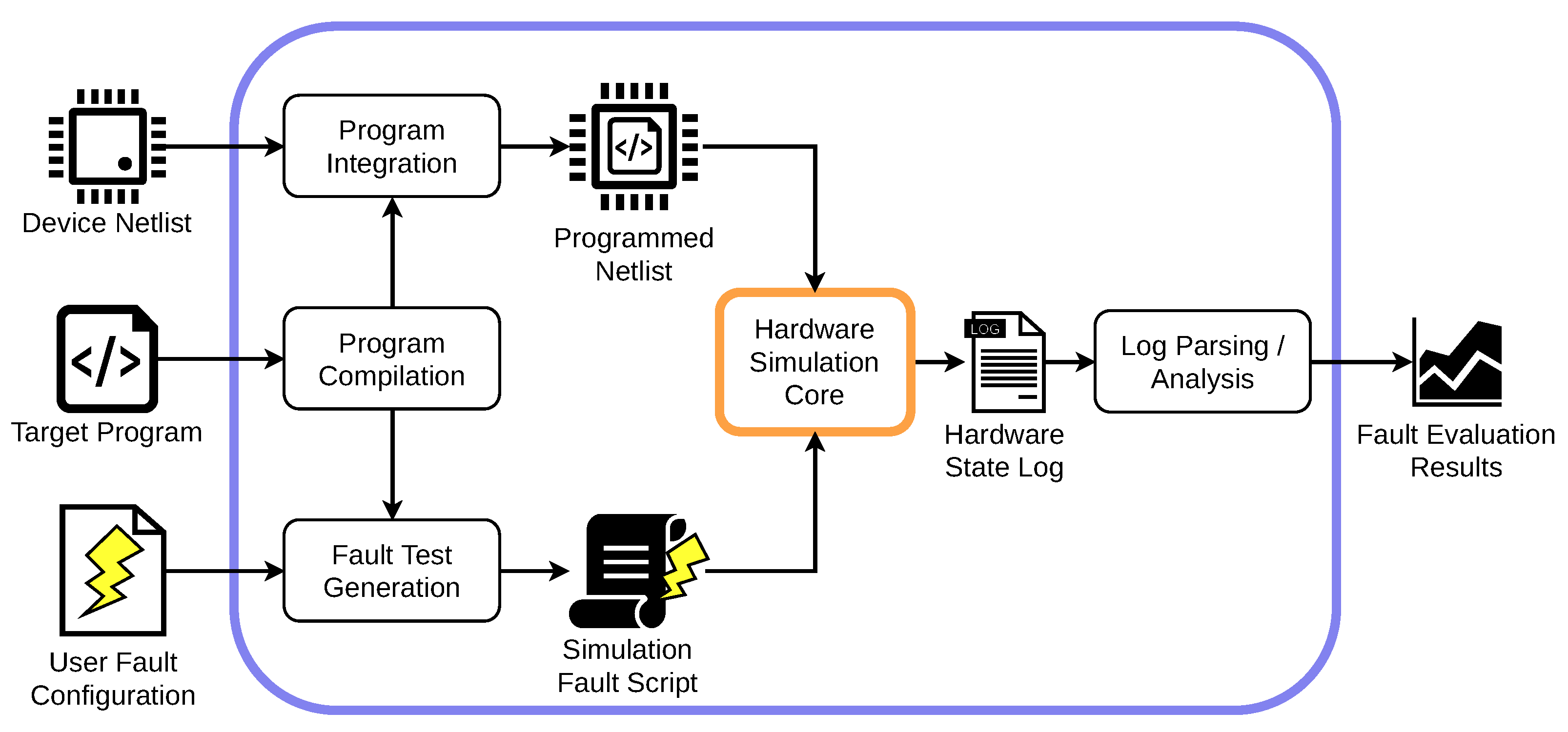
As shown in Figure 2, SimpliFI consists of two main parts: an outer test layer and inner hardware simulation core. The hardware simulation core runs gate-level simulations of the post-layout netlist and collects hardware-specific fault injection results, while the outer layer supports software-level analysis and test management. This hierarchy mimics the nature of the hardware–software relationship; in reality, software is just an advanced configuration of the hardware, and the hardware is the entity that does computational work. The inner and outer layers of the framework together support analysis of both simple instruction sequences and full programs. Evaluating short instruction sequences can aid the user in characterizing general fault vulnerabilities in the embedded processor, which is akin to studies that use physical testing to characterize a device’s fault response behavior [12]. However, SimpliFI adds another dimension to characterization results by analyzing how faulty bits manifest and propagate through the hardware. Testing full applications aids the user in evaluating realistic fault vulnerabilities in critical security software. Examples of these two uses for the framework are discussed in Section 4. For the purposes of this study, SimpliFI is only tested and implemented for evaluating clock glitch faults. However, Section 3.1.2 discusses how additional injection techniques can be modeled in the same framework.
3.1.1. Outer Framework: Software-Centric Control
The outer layer of SimpliFI is responsible for building the device simulation environment for a specific program, generating a complete set of fault test cases, and analyzing data collected during simulation. The first step of the outer framework compiles user test programs into binaries that can run on the embedded processor. To support both instruction sequence and application testing, SimpliFI accepts either a main assembly file or main C program file. The exact compilation process is highly device and program dependent and is therefore left as an implementation detail. Regardless of compilation style, a compiled binary of the program is necessary for simulating the target platform running the test program. Integrating the program with the simulated netlist is also platform dependent. In some cases, this may need to be an extra step in the simulation build process, while in other cases the program may need to be loaded during the simulation phase. An example where the dedicated integration step is necessary is when an FPGA-based processor stores a program in an internal memory primitive, such as Xilinx Block RAM [22]. The SimpliFI prototype implemented for the BRISC-V platform in Section 3.3 uses simulation build-time scripting to handle this program storage format.
Test Automation
Automated fault simulation is a key feature of SimpliFI, allowing users to fully configure multiple fault injection tests on selected program target points. To increase the flexibility and impact of the simulation framework, SimpliFI supports test configurations that inject a range of faults on multiple target instructions and even supporting fault simulation on specific pipeline stages during instruction execution. To clarify the difference between user-designed tests, program target points, and individual fault injection events, we adopt the following terminology:
- Test—A user-defined program and configuration pair that instructs the framework to test different fault injections at multiple points in the target program. A test may encapsulate multiple subtests.
- Subtest—A subtest is one part of a larger test case which specifies a start point, target point, and multiple fault injection trial parameters. The target and start points are described below, and take different meanings when testing instruction sequences vs full applications.
- Fault Injection Trial—A singular execution of the test program with one fault injected during a specific clock cycle.
The outer layer of the framework creates a fault simulation script for the simulation core which specifies all of the fault injection trials that must be run. The simulation core expects a full specification of the following parameters for each subtest:
- Program Type,
- Start Point,
- Target,
- Observe Point,
- Starting Glitch Period,
- Ending Glitch Period, and
- Glitch Period Step.
The three parameters related to the clock glitch width hold the same meaning for instruction and application tests, while the other parameters vary in purpose for the two test types. In an instruction test, the start point parameter indicates the memory address of the instruction being evaluated, and the target parameter specifies the instruction execution cycle that should be faulted. This allows the user to create multiple subtests to evaluate the fault response of different processor pipeline stages. In these tests, the observe point specifies the number of clock cycles after the start point when the instruction output should be recorded. For most instructions, this is the number of clock cycles required to process the instruction. However, since the full device memory is not recorded by the simulation core, the observation point could be set to a later time in the case of memory store instructions, where the value written into the memory can be read back into a processor register for observation.
Since applications have significantly more complicated program flow than a short sequence of instructions, the address of an instruction is not a sufficient identifier for when the simulator should inject a fault. Instead, the test program can be instrumented using a unique macro or function that is called when the simulator should prepare to inject the fault. In this case, the start point parameter identifies the memory address of the macro, and the target identifies where the target instruction is following the macro. The observation point is determined in a similar method to the start point.
To simplify user configuration of the simulation tool, SimpliFI defines a custom and flexible file format for the user to specify test configurations. Instead of fully specifying all parameters for every subtest, the user can set global parameters that apply to every subtest, and then create shorthand entries for different instruction and cycle subtests. Before SimpliFI starts the simulation core, it converts the user configuration file into a fully-specified fault simulation script that the simulation controller can understand. An example user configuration file is provided in Listing 1, where the GStep, GStart, GEnd, Observe Point, and test type are set for all subsequent subtests. With the “@@” characters acting as subtest delimiters, this configuration file will create subtests for the instruction at address 2C for stages 0 through 7, and the same for the instruction at address 4C.

Listing 1.
Sample user fault configuration file.
| SEQ |
| GStep: 0.5 |
| GStart: 12 |
| GEnd: 4 |
| ObservePoint: 7 |
| StartPoint: 2c |
| Target: 0,1,2,3,4,5,6 |
| @@ |
| StartPoint: 4c |
| Target: 0,1,2,3,4,5,6 |
| @@ |
Output Processing
SimpliFI analyzes both hardware fault propagation and software-level outcomes by leveraging the hardware state information recorded during simulation. The post-processing performed on the data supports the same types of analyses as physical device testing, where program and instruction outputs are inspected for errors. For instruction sequences, the goal of post-processing is to determine how the instruction output and hardware state are impacted by different fault parameters, with faults being injected at different stages across multiple subtests. SimpliFI computes the Hamming distance (HD) between actual execution outputs, and the expected values observed during a clean run of the same program. The HD analysis identifies all registers that were corrupted in at least one subtest and calculates how each fault injection trial affects the final value. For full application tests, the same final register data is collected as in the instruction tests, but only the registers which hold program outputs are used to determine the application-level impact of fault injections.
Although its focus is on program-level effects, SimpliFI can analyze how fault propagation through the hardware state corresponds to different program outcomes. While some software-level corruption may primarily be the outcome of software-level error propagation, it is possible that some software outcomes consistently correspond to the same types of hardware-level fault propagation. These main analysis features are only a starting point for the output processing stage, and users can implement their own metrics and analytic methods to extend the results of the SimpliFI framework.
3.1.2. Inner Framework: Hardware Simulation Core
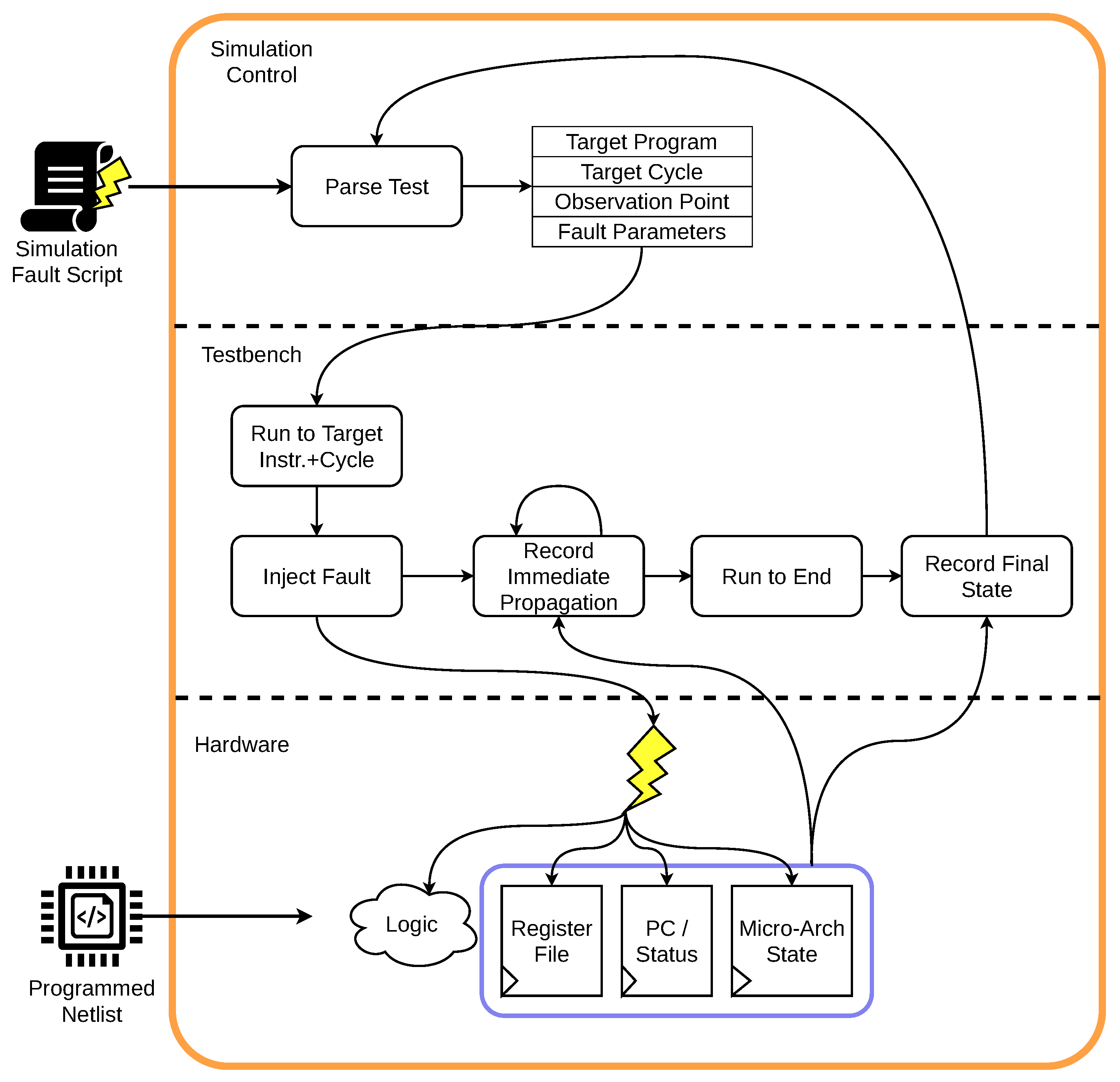
The inner layer of the SimpliFI framework is responsible for injecting faults into the simulated hardware and tracking the hardware state both immediately after the fault and at the end of execution. This is accomplished through a post-layout netlist simulation testbench along with an extra level of control scripting that interprets test cases as shown in Figure 3.
By using post-layout gate-level simulation, SimpliFI incorporates timing properties of the device signals into simulated fault manifestation. There are numerous hardware simulation tools that support physical netlist timing simulations, which are developed to efficiently evaluate hardware [23,24]. While it is possible to write a custom simulator that has built-in fault support, such as VerFI, simulating with a dedicated hardware tool is likely faster and more efficient [17].
The simulation core control level is responsible for reading each subtest configuration and loading the parameters into the hardware testbench. Modern hardware simulators support testbench intervention like this at runtime, allowing the simulator to be invoked once and restarted multiple times to run different fault injection trials. Before running the fault injection trials, the controller runs an initial clean test for each configuration to gather the expected values and runtime. This baseline data is necessary for effective fault response analysis during output processing. The testbench functionality shown in Figure 3 can be achieved with a SystemVerilog testbench which supports high-level modules reading values from lower levels of the simulated hardware. This feature allows the internal state to be recorded at arbitrary time points during simulation.
3.2. Fault Modeling
A critical part of SimpliFI is its ability to inject realistic faults into the hardware. As stated earlier, this study focuses on simulating clock glitch fault attacks, although other injection mechanisms can be simulated as well. By using gate-level simulation, the timing information required to emulate clock glitch attacks is automatically included in the simulated netlist behavior. During gate-level simulation, gate outputs are updated according to their propagation delays defined in an SDF file.
With signal propagation time enforced by the simulator, the testbench can emulate a clock glitch by manually shortening the clock period for one cycle and then returning to the correct clock frequency. If the period is not short enough to violate signal timing, no faulty bits are latched into the registers and the simulation will continue to run as if no fault was injected. However, if the clock period does cause timing violations, then faulty bits may manifest in the hardware state and propagate through the program. While any violation of the critical path constitutes a successful clock glitch event, the resulting faulty bits are caused by two distinct timing events.
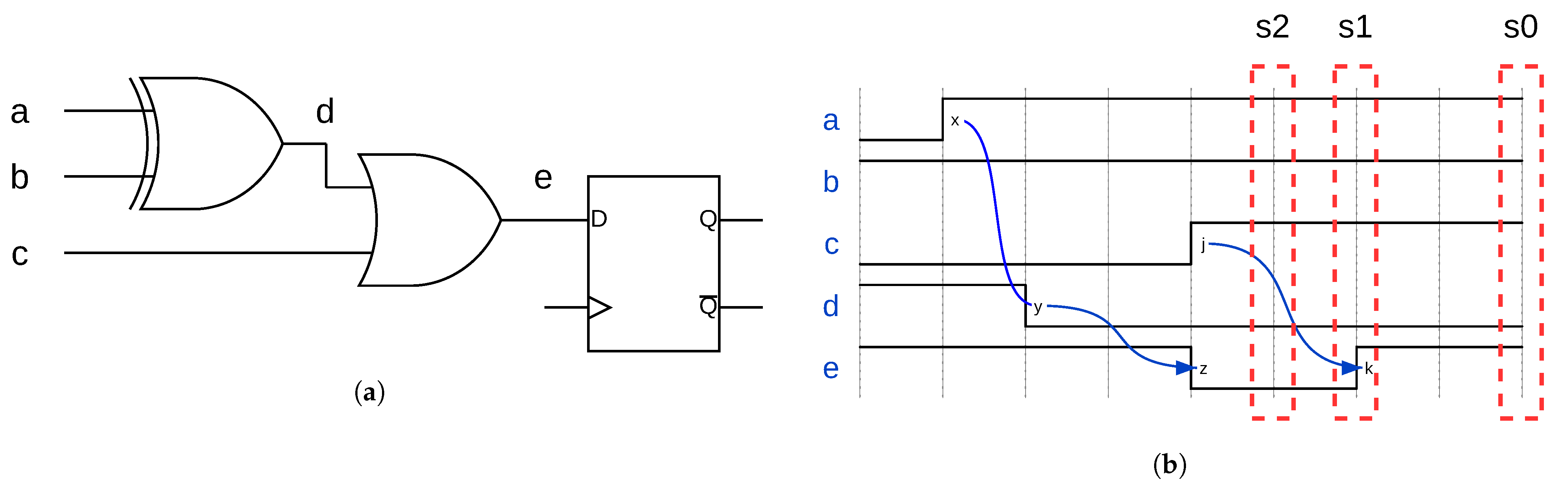
To demonstrate the two event types, consider the circuit shown in Figure 4a. The XOR and OR gates both have propagation delays from input to output, which for the purposes of this example are just considered to be greater than 0 nanoseconds. The timing diagram in Figure 4b shows signal propagation in response to the input changing from to , with a transitioning before c. If the clock edge occurs at the end of the s0 window in Figure 4b, the correct e value is latched into the register. If the clock edge occurs at the end of the s1 window, a setup time violation occurs due to e transitioning during the setup windows. In this case, the register state is unpredictable and may even become metastable. Finally, if the clock edge occurs in s2, there is no setup time violation since the data does not change in the sampling window. However, the temporary 0 value on e will be latched into the register. While both of these events count as timing violations, one of them violates the setup time, and the other causes an early incorrect sample.
Hardware simulators naturally handle incorrect sampling events, since the propagation delays are modeled correctly so that signal e appears as a 0 at sampling point. However, the setup time violation event is more complicated since setup time violations in a real circuit can lead to register metastability. Current metastability models rely on analog characteristics of the register and data signal to characterize metastable flip-flop outputs with some level of accuracy [25,26,27]. Since digital gate-level simulation abstracts away the underlying device physics, there is not enough information to simulate potential metastable behavior using the existing models.
However, SimpliFI supports a random metastability model as a best effort to simulate setup time violations. Instead of latching the data signal value at the exact time of the clock edge, a random value is assigned to the register state. While metastability is not a fully random phenomena, this technique acknowledges that unpredictable values may be introduced into the hardware state as a result of clock glitches that cause setup time violations. This random model has been used before as a technique for acknowledging metastability in digital simulations [28].
Injection Mechanism Extensions
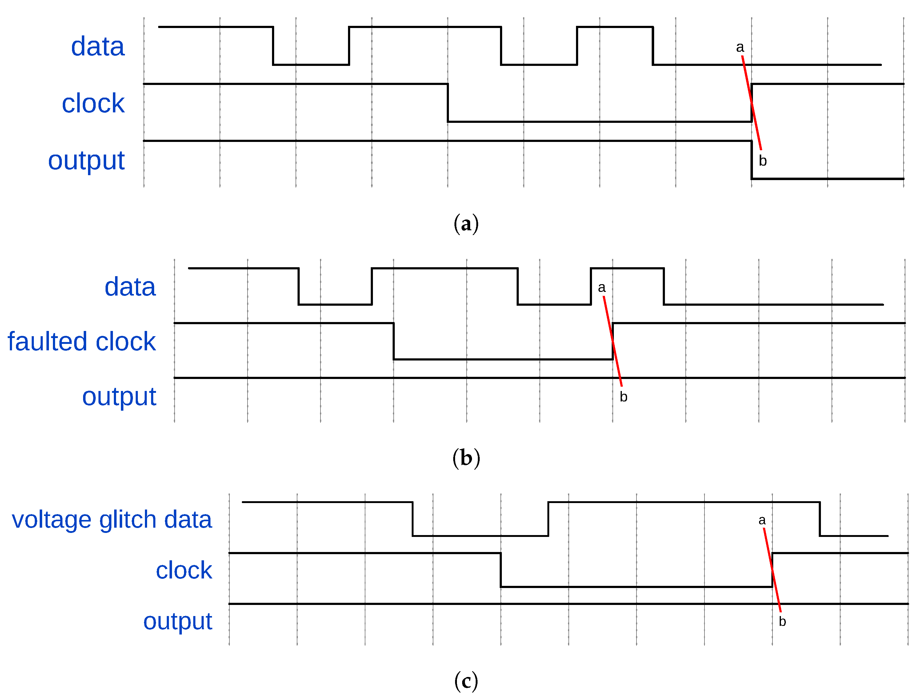
The underlying physical effect SimpliFI leverages for fault injection is timing violations, with the injection technique being a clock glitch. Therefore, other timing-based faults could be added to the framework for future extensions, including voltage-based faults and even EM faults. Similar to clock glitch faults, voltage-based faults also disrupt circuit timing to inject errors into the state. Figure 5 shows example clock and voltage glitch fault effects on a register. A voltage glitch attack increases the propagation delay of data signals, leading to longer critical paths. Figure 5c shows this, with the normal data transitions from the clean sample taking a longer amount of time to update in the faulted version. In this example, the clock and voltage glitches can lead to setup time violations or critical path violations. In both cases, the rising clock edge occurs closer to the data transition times; the clock glitch moves the clock edge closer to the data, while the voltage glitch moves data transitions closer to the clock edge.
These shared properties are one potential way to achieve voltage glitch simulation in the SimpliFI framework. The clock glitch mechanism already moves the clock edge closer to the data transitions, and could be used in the same way to simulate voltage glitches. The key challenge that needs to be addressed is calculating how the clock glitch width maps to a particular voltage glitch. More work would be required to determine this relationship, but this is a potential starting point for supporting more injection techniques. Voltage underpowering attacks have similar effects as voltage glitch attacks, so the mechanism for voltage glitches could be applied for a longer period of time to simulate voltage underpowering. While EM faults are more complicated than clock and voltage attacks, the underlying fault manifestation is caused by setup time violations with data signals at the positive supply voltage [29]. Since SimpliFI already supports basic metastability modeling in setup violations, EM faults could be integrated into the framework by modifying data signals in the device that would realistically be affected by EM pulses. This is one extension for future work on SimpliFI that would greatly increase the versatility of the framework beyond its current abilities.
3.3. Integration in Embedded Flow
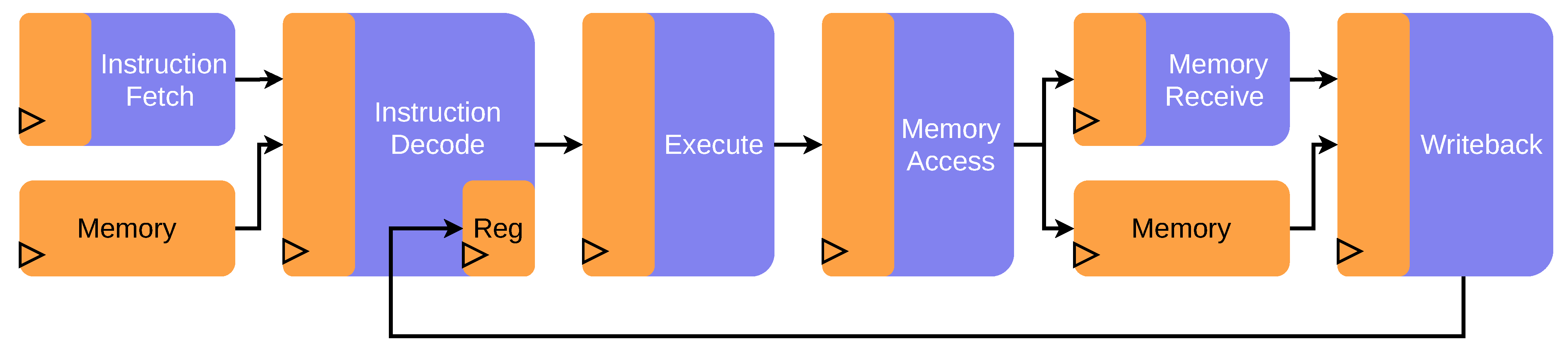
We implemented SimpliFI for the BRISC-V platform created by the Boston University Adaptive and Secure Computing Systems Lab [5,6]. This implementation demonstrates a practical integration of the SimpliFI methodology into an embedded toolchain, but the generic, high-level framework is suitable for other platforms as well, regardless of the particular development tools. To apply SimpliFI to another device, a gate-level netlist would be required in addition to changes in the BRISC-V implementation scripts. BRISC-V is an open-source RISC-V processor platform that allows users to customize a processor implementation with different pipeline lengths, memory hierarchies, and memory sizes. The customization used for the SimpliFI prototype had a 7-stage pipeline and a single memory that stores both the program code and data. Figure 6 depicts the selected processor pipeline.
We implemented the BRISC-V processor for Xilinx FPGAs, and developed the framework implementation around the Xilinx Vivado Design Suite. When building the BRISC-V processor in Xilinx Vivado, the original netlist did not utilize Block RAM due to an incompatible memory access process in the Verilog code. To bypass this and achieve a netlist that uses Block RAM for memory, we modified the original memory access code to match the Xilinx memory inference template. The main functional difference between these two versions is that when the memory is written to, the write value propagates to the output bus. This did not cause any execution errors when testing large applications to verify validity. Otherwise, the changes to the enable logic preserve the original behavior, but by using only one if statement per port as required by Vivado Block RAM inference.
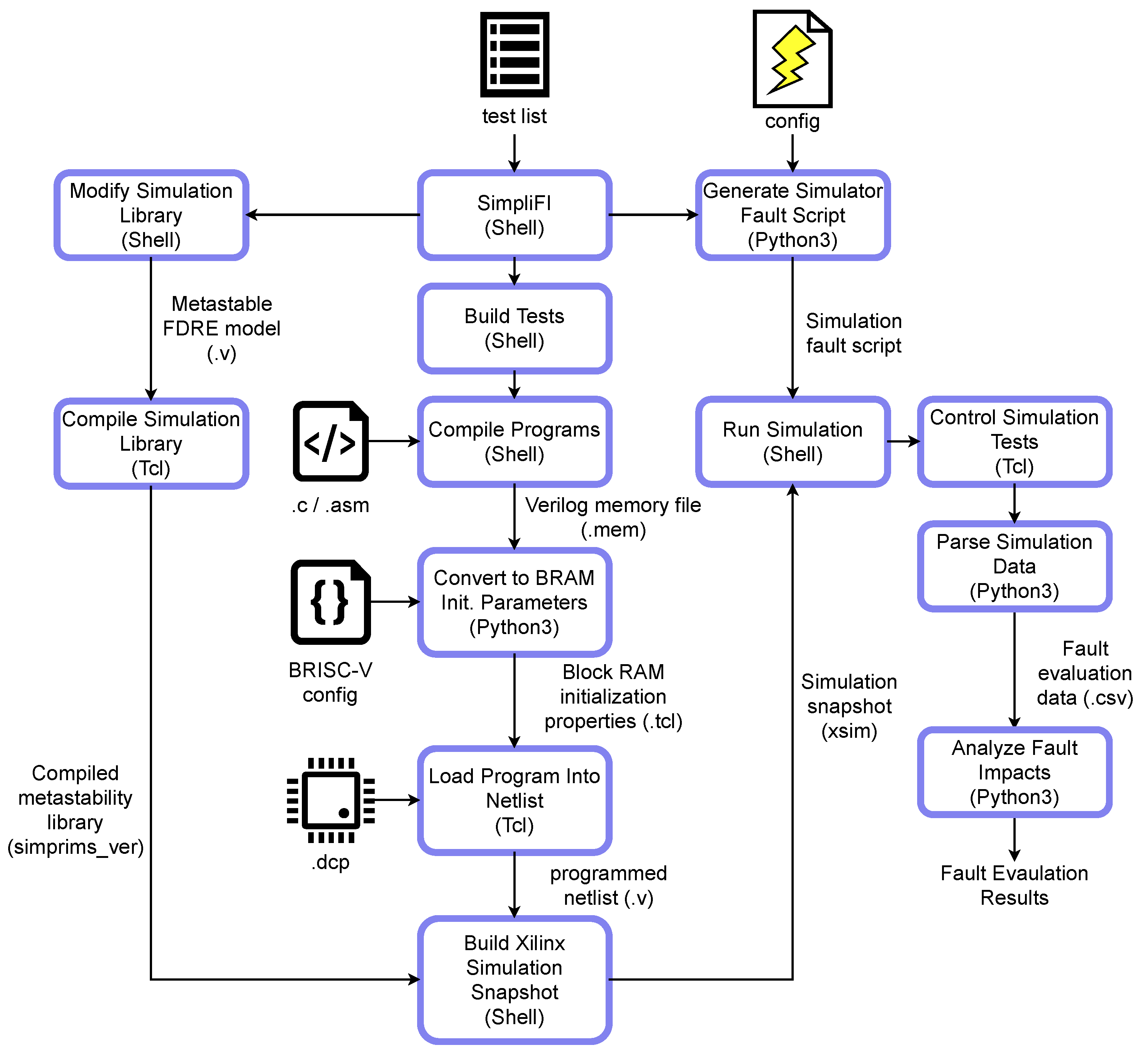
Figure 7 depicts the various steps in the SimpliFI tool flow that work together to build an automated simulation environment for user test cases. One critical phase of this flow is the process of converting a user test program into a Xilinx simulation snapshot. This implementation of SimpliFI uses a series of scripts to convert the compiled binary into Xilinx Block RAM initialization parameters, which are then applied to a copies of the post-layout netlist to produce device images that have the exact same circuit but different programs loaded in them. By doing this, SimpliFI ensures that the software evaluation results for all test cases accurately represent realistic fault responses of the original device netlist provided by the user.
4. Results
We used SimpliFI to characterize software fault vulnerabilities of programs running on the BRISC-V processor synthesized and implemented for the 28 nm programmable logic on the Xilinx Zynq xc7z020clg484-1 device. Therefore, the detailed fault response data is dependent on the particular propagation delays for the specific processor layout and device timing properties. We characterize the fault response at two levels: the instruction level and the application level.
4.1. Characterization at the Instruction Level
Using simple instruction sequences to characterize an embedded processor’s fault response has been shown to be an effective technique during physical device testing [10,11,12]. SimpliFI supports this technique, and provides benefits over physical testing by enabling rapid evaluation through simulation and collecting hardware state information during execution. The goal of this type of evaluation is to build a knowledge base or model of how any type of instruction may be vulnerable to fault attacks. Therefore, all aspects of an instruction are of interest: opcode, addressing mode, operands, data, etc. An evaluator generally wants to know how each of these instruction components contribute to overall fault response. Acquiring this information essentially provides insight into how the hardware that implements each component is vulnerable to fault attacks. To fully characterize a device, tests are designed to isolate microarchitectural components to evaluate their fault responses, and to generalize the common fault vulnerabilities and behavior exhibited by instructions with similar parameters.
To demonstrate SimpliFI’s instruction characterization capabilities, we characterize ADD, LW (load word), and JALR (jump-and-link with register) instructions from the RISC-V 32 bit integer ISA (RV32I). These three instructions together represent the range of capabilities on a load-store architecture, where most instructions are categorized as performing arithmetic and logic, memory access, or control flow functions. Although these three instructions are representative of the full ISA, the same analysis can be performed for all instructions. Within each instruction, the effect of different destination registers, source registers, source orderings, register values, and immediate values are evaluated. To do this, a separate test is created for each instruction component that isolates the behavior for the component of interest. To test fault effects on the destination register, we simulate faults on multiple copies of the same instruction with varying destinations. The same approach is used for the other components of interest. For the purposes of this evaluation, the following terms apply:
- Instruction Component—A portion of the specification for an instruction executed by the processor. Examples of instruction components include the destination register, source registers, and immediate values.
- Instruction Test—A collection of SimpliFI tests that help characterize the behavior of a specific instruction in response to different fault attacks.
- Instruction Component Test—A specific SimpliFI test that is designed to isolate the impact that different microarchitectural blocks have on the instruction fault response by changing one component of the instruction.
- Fault Response—The behavior of faulty bits in the processor in response to different fault attacks. The results may refer to the fault response of the hardware state as a whole, or of the test outputs. For the test outputs, response is usually qualitatively defined in terms of how the number of faulty output bits changes as a function of the fault injection parameter. For example, a monotonic output response means that, in general, the number of faulty bits in the outputs consistently increases or decreases. An oscillatory output response means that the number of faulty bits alternates between high and low counts as the clock glitch width changes.
- Fault Sensitivity—The range of clock glitch widths which induce erroneous bits in the fault response. This term can apply to both the hardware state fault propagation and the test outputs.
- Fault Intensity—The number of errors induced in the fault response by a fault injection attack. This term can apply to both the hardware state fault propagation and the test outputs.
For each instruction component test (e.g., destination and source 1), 4 instances of the same instruction with varying selections of the target component were evaluated. To evaluate each of these components using SimpliFI, a unique test program was written for each instruction component. Listing 2 provides the specific test programs for evaluating the impact of the first source register in ADD instructions. The target instructions are padded with NOPs to ensure previous and future test setup instructions do not interact with the target instruction execution. Furthermore, each subtest was conducted with faults being applied at each execution stage, with clock glitch widths ranging from 12 to 2 nanoseconds in 250 picosecond increments.
ADD Instruction
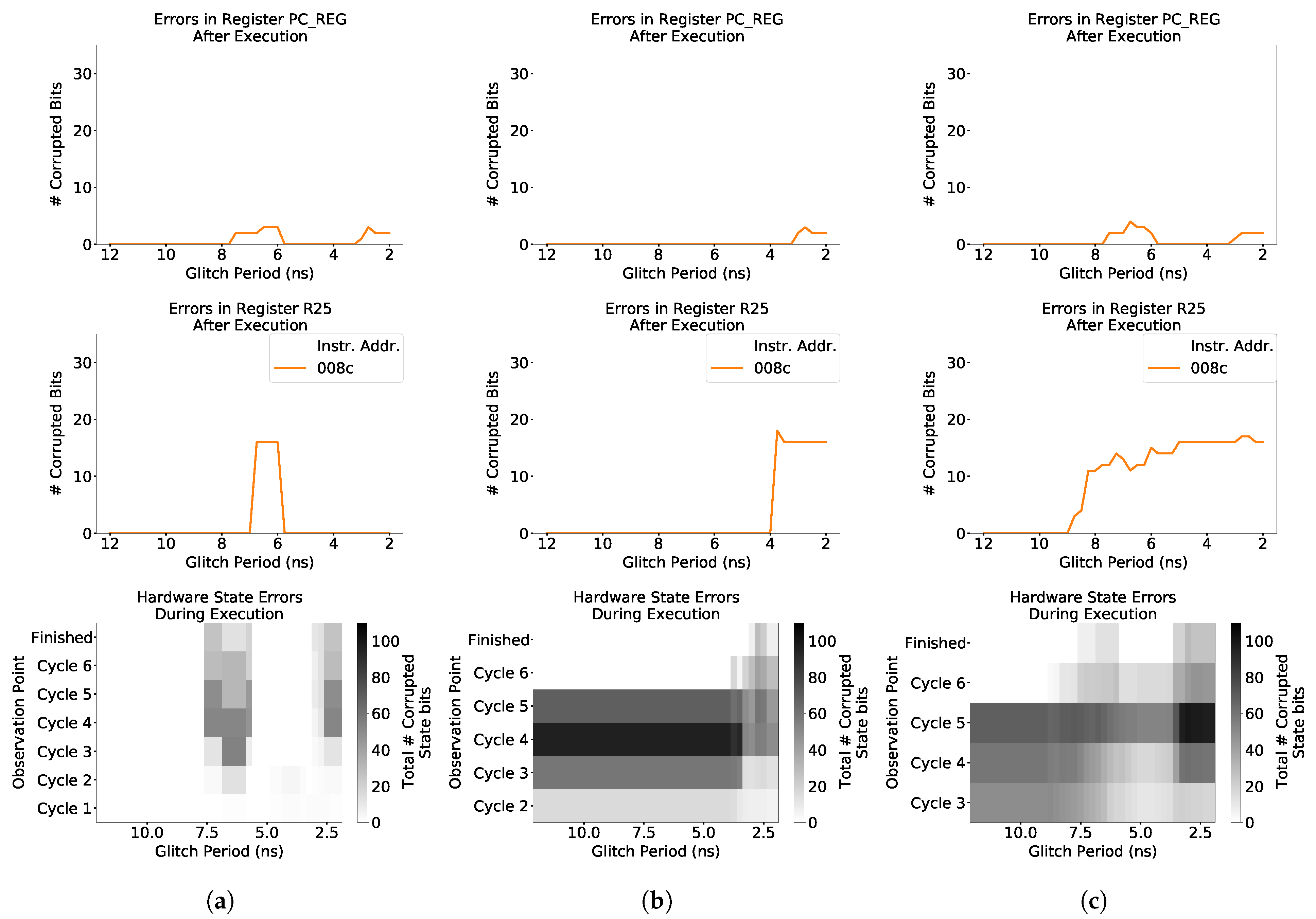
Figure 8 shows the results from injection clock glitches during different stages of an ADD instruction. The fault evaluation analysis calculates the Hamming distance (HD) between the results of clean simulations with no faults and the results of fault injection trials. The top graphs in Figure 8 and subsequent figures plot the number of faulty bits in the output register in response to multiple clock glitch widths. The bottom heatmaps depict how the number of faulty bits in the entire hardware register state changes as the instruction executes. In each heatmap, the lowest point on the vertical axis shows the number of faulty bits in the cycle immediately following fault injection, and time proceeds up the vertical axis until the instruction finishes execution. Since the state only contains faulty bits after the fault is injected, previous cycles of execution are omitted from the heatmaps. For example, the hardware state fault heatmap in Figure 8c starts at execution cycle 3 since the fault was injected during stage 2.
Listing 2.
An example instruction sequence test program that focuses on evaluation of the ADD source 1 instruction component.
Listing 2.
An example instruction sequence test program that focuses on evaluation of the ADD source 1 instruction component.

The instruction output plots in Figure 8 show that the impact of identical faults on the instruction output varies depending on when the fault is injected. When faults are injected at the beginning of execution in stage 0, only clock glitch widths between 7.25 and 5.5 ns result in corrupted output data. However, faults injected in stage 2 affect instruction output as long as their glitch widths are shorter than 10.5 ns. The instruction fault responses give an indication of how different faults will affect software execution since the instruction outputs are ultimately relevant to software behavior.
The hardware state fault propagation heatmaps instead give insight into how faults affect processor execution even when they fail to affect instruction outputs. The hardware state fault propagation plots in Figure 8 always exhibit erroneous bits remaining in the circuitry up until the end of execution where corrupted output data appears in the registers. For example, a high volume of state corruption can be seen throughout execution in Figure 8a in response to faults that cause corrupted outputs. Glitches in the range of 7.75 to 5.75 ns induce hardware state errors that propagate through to the output, although only glitches shorter than 7.25 ns affect the data registers and glitches between 7.75 and 7.25 ns only affect the program counter. There is also significant error propagation from glitches shorter than 3 ns, which only affect the program counter by the end of execution.
However, attacks during stages 1 and 2 have significantly different effects on the hardware. Figure 8b,c show that every tested glitch width resulted in at least 50 corrupted state bits within the third subsequent execution cycle, but that the glitches applied in stage 1 result in up to 85 state errors. However, none of these errors propagate to the data outputs, and only 7.75 to 5.25 ns glitches in stage 2 resulted in program counter errors. Another fault behavior in these results is that certain faults induce few errors during injection, while others induce significantly many errors. One trend shown by all of the hardware fault propagation heatmaps is that glitches resulting in few immediate errors tend to cause amplified state corruption a few cycles later. These gradually amplifying faults seem to have the greatest impact on instruction outputs. Conversely, faults that immediately cause significant state error suddenly disappear two clock cycles before the end of execution.
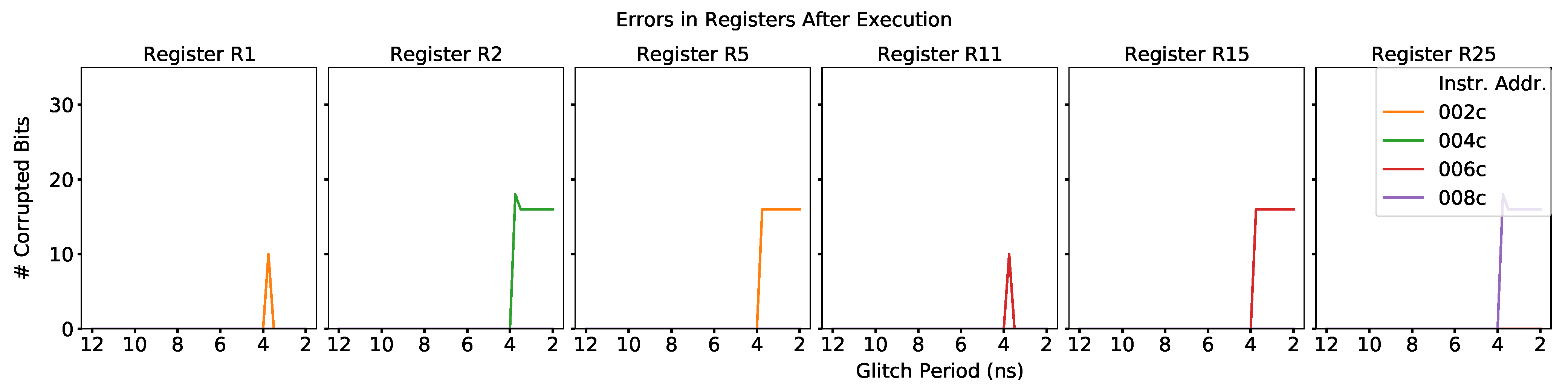
In most of the tests, only the targeted destination register and the program counter are affected by fault injection. However, clock glitches with 4.25 ns widths applied in stage 1 not only affect the target destination register, but other registers as well. This is shown in Figure 9, where faults were injected on the instruction decode stage of multiple ADD instructions each targeting a different destination register. The instruction targeting register R15 also modifies R11, and the instruction target R5 modifies R1. This behavior was only observed in response to faults during stage 1. Furthermore, the final erroneous bits in the destination registers vary slightly from one instruction to another. For 4.25 ns glitches injected in stage 1, instructions targeting destinations R2 and R25 result in slightly more erroneous bits. These anomalous behaviors for stage 1 faults call attention to the underlying circuitry for the pipeline stage. It may or may not be a coincidence that targeting registers R5 and R15 results in corrupted values in registers R(5−4=1) and R(15−4=11), while targeting R2 and R25 results in additional corruption in the intended destinations for the exact same fault attack. The important observations here are that (i) data can be written to the wrong destination register, and (ii) that the selected destination register has a minimal but non-zero impact on the faulty bits that propagate to the end of execution.
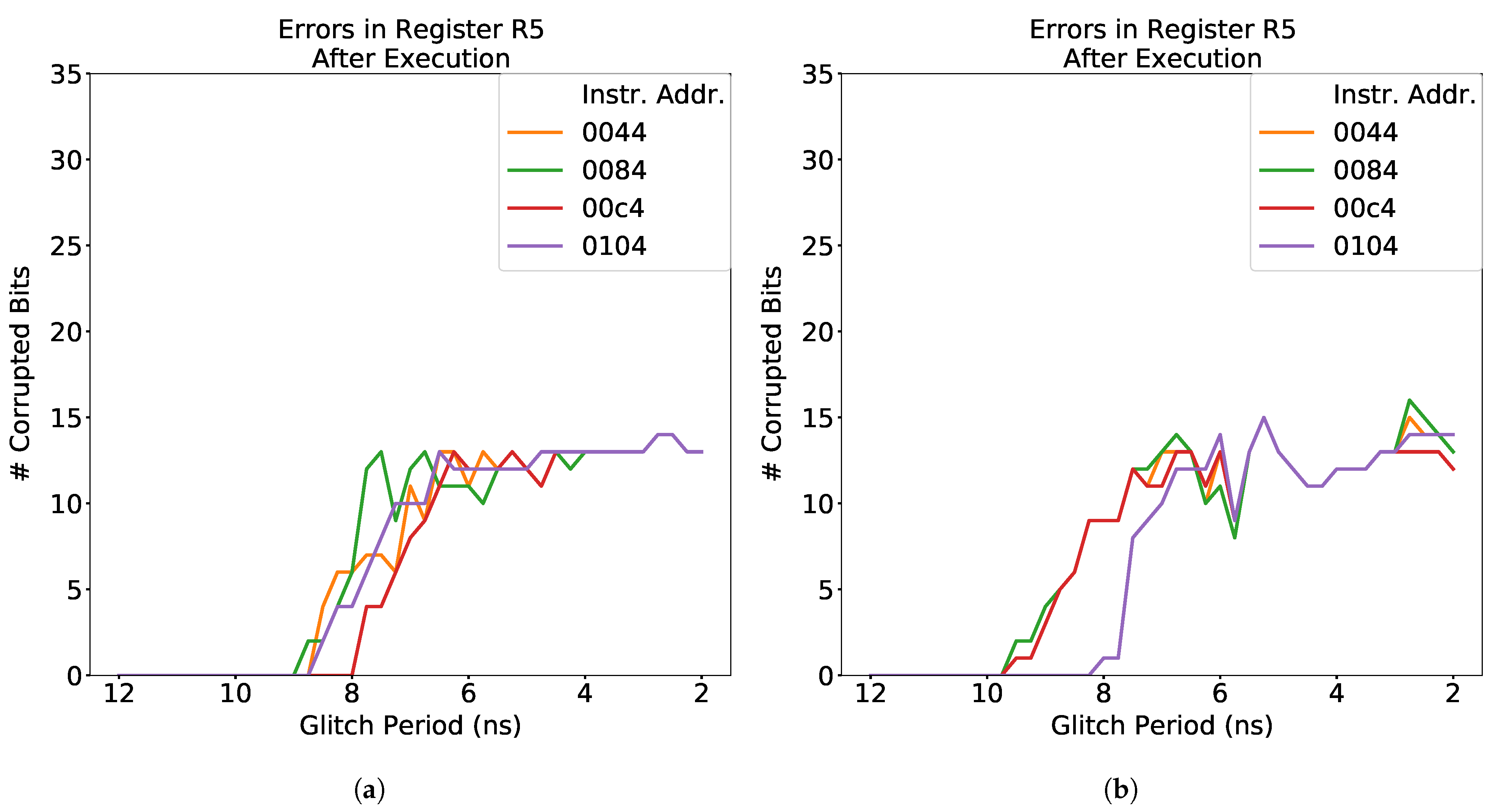
When testing different source registers, SimpliFI revealed that the selected source register has a greater impact on faulty instruction outputs compared to the destination register. The impact from faulting the instruction decode stage of ADD instruction induced the response shown in Figure 8c for all destination register selections. However, the responses for the same exact faults vary when selecting different source registers, as shown in Figure 10. While the responses have similar monotonic structures, the exact number of faulty output bits changes depending on the first source register. The impact of the second source register is lesser than the first. However, the instruction using R2 as the second source register was not affected by 10 to 8.25 ns glitches (Figure 10b).
Furthermore, the first and second source registers’ impacts on the fault response exhibit opposite behavior at the extreme ends of their fault sensitivity ranges. In Figure 10a, fault responses to glitches longer than 4 seconds are influenced by the first source register, while Figure 10b shows that responses to glitches shorter than 3 ns are influenced by the second source register. The different fault responses observed when testing different source 1 and source 2 operands indicate that the hardware that either pipelines the source selections or that propagates values from the source register to the ALU is unbalanced. The hardware for source 1 appears to be more sensitive since fault responses fluctuate significantly more when targeting the first source operand compared to the second. However, the logic paths that select R2 for the second source may be unbalanced as indicated by the different fault sensitivity shown in Figure 10b.
LW Instruction
Results from testing the LW instruction showed that different classes of instructions have unique responses to fault attacks. Unlike the ADD instruction, faults during the instruction fetch did not result in faulty outputs for the LW instruction, and the fault responses to attacks during the instruction decode varied between the two classes. Even though the same destination and source registers were selected for both classes, the way that the microarchitecture handles decoding of the two instruction types leads to different instruction fault responses. In particular, faults on the decode stage of LW instructions corrupted more than one unintended register in some cases, where faults on the ADD instruction corrupted at most one additional register. Additionally, the LW exhibited vulnerabilities to faults during the memory receive stage (stage 5) of the BRISC-V pipeline, which was not a vulnerable stage for the ADD instruction. This is expected since arithmetic instructions do not require further memory access after the instruction fetch. One unexpected microarchitectural effect was revealed in the LW results, where the first instruction had a different output fault response than subsequent sections. When store instructions were placed in between the target LW instructions, all tested instances of the LW instruction exhibited nearly-identical fault responses.
JALR Instruction
Testing the JALR instruction demonstrated further impacts of the microarchitecture on instruction fault responses. The JALR instruction computes the target program execution address by adding an immediate value to an address obtained from a source register, and also stores the return address in a selected destination register. The fault response of the program counter matched closely with the fault response of ADD instruction destination registers for faults injected during the instruction decode and execute stages. This is likely because the ALU is used in similar ways during ADD and JALR registers. For example, both of these instructions obtain their first operand from a source register during the decode, and use a similar add operation to compute their final value. On the other hand the fault response of the return address destination register in JALR instructions was similar to that of the ADD destination register for faults during the instruction receive stage, but not during the decode or execute stage. This behavior is also attributable to the microarchitecture, where the ALU used in the execute stage has logic for computing the return address which is separate from the logic for adding two full operands together. Finally, the destination registers for both of these instructions share the exact same fault response for faults during the writeback stage (stage 6), since the only event that happens is the final value being written into the destination register.
The raw program counter values collected from the JALR test results indicated exactly how flow control could be violated using fault attacks. Faults during the instruction fetch induce faulty bits in the hardware state but they do not propagate to the new program counter value. In general, the precise timing of a fault during the instruction decode stage determined the type of effect that the fault had on flow control. Some faults resulted in skipped jumps, which is in line with traditional models. Other faults reset the program execution to start at address 0, after which the processor would sometimes successfully complete the original jump, but other times remain at the program start. The former case is previously unobserved behavior which would enable an attacker to execute instructions from the start of the program, but then allow the program to continue executing from the originally-intended function address. Finally, the remaining instruction decode faults resulted in other non-zero corruptions of either the target address, return address, or both.
Summary
A high-level summary of each instruction’s susceptibility to faults injected in different stages is given in Table 2, and the impact of each component (destination, source, immediate value, etc.) on the fault response is summarized for all three instruction types in Table 3. SimpliFI is able to provide detailed information about how any fault applied during execution will affect instruction behavior by analyzing both the hardware fault propagation and final instruction outputs. The tests discussed in this section provided more fault response information than has been obtained with other techniques, and in some cases highlighted fault outcomes that are rarely seen in practical fault studies.
4.2. Characterization at the Application Level
SimpliFI is also able to characterize the effects of faults on full applications running on the target platform. The goal for application-level characterization is determine broad effects that a given fault will have on the program. Traditional software-level fault outcome characterizations place faults into three main categories based on their program-level effect:
- Unsuccessful Fault—The fault caused no change in program behavior.
- Fatal Error—The program crashed.
- Successful Fault—The program produced faulty outputs.
However, SimpliFI’s access to hardware-level fault propagation enables deeper insight into how the fault affects the processor evern when the application is not affected. Therefore, application-level characterization with SimpliFI expands the possible outcome categories to consider 6 different behaviors:
- Silent Fault—The hardware state was not affected by the fault.
- Unsuccessful Fault—The hardware state was affected, but the fault caused no change in program behavior.
- Fatal Error—The program did not complete within 500 clock cycles beyond the expected execution time.
- Output Corruption—The program produced faulty outputs.
- Time Difference—The program execution time was different than expected, but no outputs were affected.
- Output and Time Corruption—The program both produced faulty outputs and executed in an unexpected number of cycles.
We present the characterization of an Advanced Encryption Standard (AES) program running on the BRISC-V processor. Differential Fault Analysis (DFA) attacks on AES have been shown to be effective for a number of points in the algorithm. Two possible points are after the first add round key operation, and during the last round of encryption before the mix columns operation [30,31]. We use the reduced t-table, unprotected AES implementation included as the reference cipher in the NIST lightweight cryptography benchmarking suite [32]. This implementation originally comes from the MbedTLS library. The code was instrumented for SimpliFI fault simulation by calling __SimpliFI_Start and __SimpliFI_Observe macros to mark the start of the injection point region and final output observation point, respectively. Two points in the algorithm were targeted: the input of the first round following the round 0 add key transformation, and at the start of the 9th round. The instructions around these points heavily consist of arithmetic and logic instructions and only 1 or 2 memory instructions, but both points in the program have a control flow instruction. Round 1 has a branch-on-greater-than instruction and round 9 has a jump-and-link instruction. Clock glitches were injected at the start of each instruction, with glitch widths ranging from 12 to 2 ns.
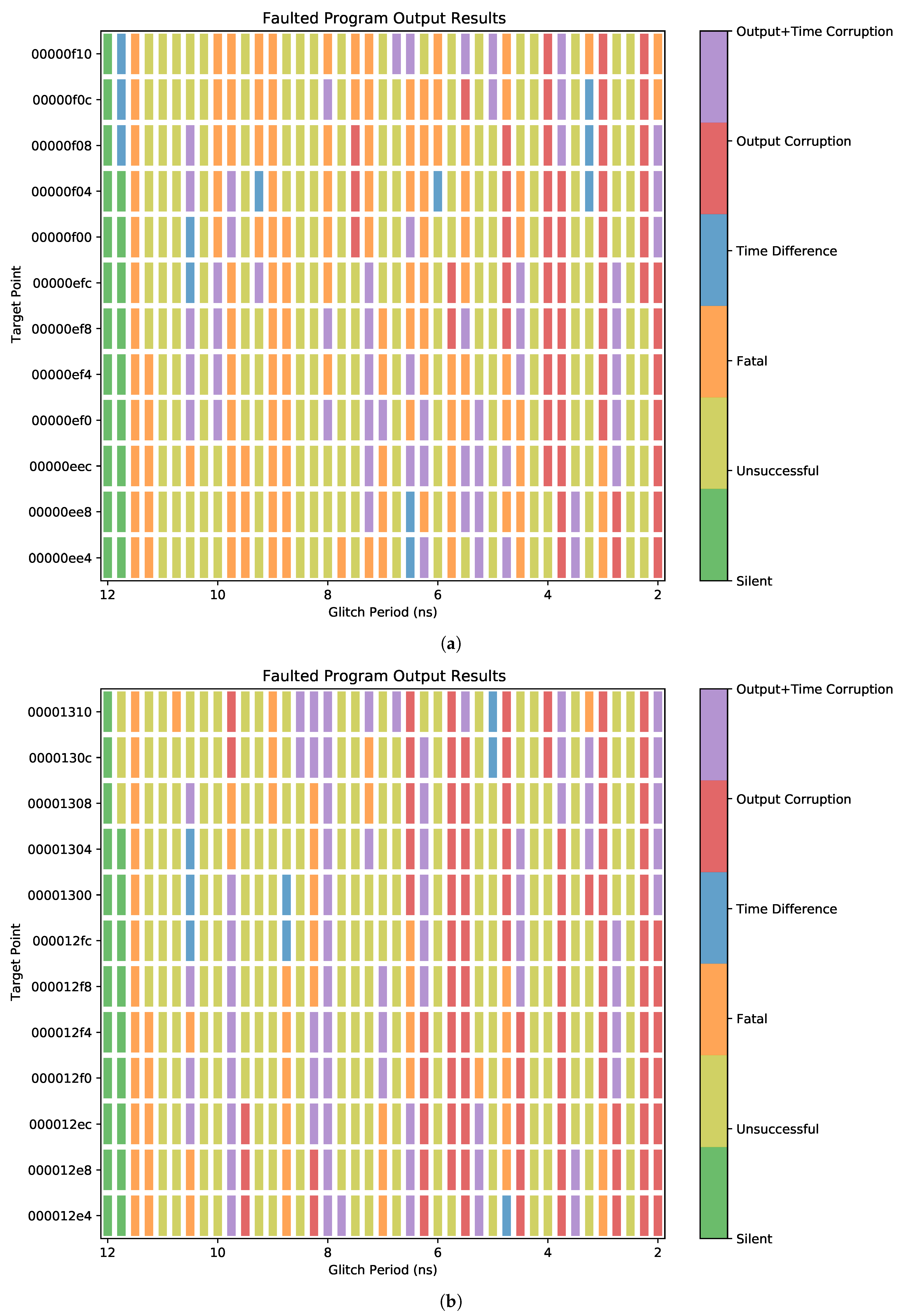
A simple breakdown of the test outcomes for attacks on rounds 1 and 9 of the AES implementation is given in Table 4. In general, round 1 attacks caused more fatal errors than round 9 attacks, while round 9 attacks caused more output corruption with and without time differences. This is intuitive from an algorithmic point of view, since faults injected earlier in the program have a longer amount of time to cause more errors throughout execution. The plots in Figure 11 show much more detail about which exact faults caused these outcomes. Comparing the vertical patterns to the horizontal ones reveals that different glitch widths tend to have similar effects on program execution no matter which instruction they were applied to. Conversely, the impact of different faults applied to the same instruction varies significantly as the glitch width changes.
The results in Figure 11 also show how the same glitches have different effects on rounds 1 and 9. While the instructions executed during each point are slightly different, there is enough similarity to compare the results. For example, the [12,10] ns range has nearly the same effect when applied both rounds, except for a few extra execution time inconsistencies and fatal errors at 11.75 and 10.5 ns. Some interesting features of how the results differ are seen at [9.75,9.5] ns and [8.5,8] ns. A two-column region of fatal errors at 9.75 and 9.5 ns in Figure 11a turns into mostly output+time corruptions in Figure 11b. However, next to this at 9.25 and 9.0 ns, another region of fatal errors turns into mostly unsuccessful faults. Similar to the first region, the unsuccessful faults from 8.5 to 8.0 ns in the round 1 tests turn into mostly output+time corruptions with a few fatal errors.
The fault responses from on round 9 faults are ideal for an attacker compared to round 1. Since the adversary wants to collect faulty outputs, the round 1 fatal errors are undesirable. In round 9, the attacker would have a greater chance of obtaining faulty outputs and less of a chance of crashing the device. This insight into the program behavior is valuable for software engineers since it can inform them about which points in the program are more vulnerable. With these results, the software engineer would likely focus more time securing the round 9 operations, and focus less on round 1 due to the high number of fatal errors. However, the software fault responses during round 1 are still pertinent for fault evaluation, particularly if the attacker may utilize fault sensitivity analysis as proposed by Li et al. [33].
5. Conclusions
With extensive research into fault attacks over the years, embedded security researchers and analysts have a strong collective knowledge of what fault attacks are capable of, and how they occur. We are at a point where this vast amount of knowledge can be integrated into automated techniques for hardware and software fault evaluation, and this study demonstrates that with the introduction of SimpliFI. Even with a simple injection mechanism, SimpliFI reveals device-specific microarchitectural effects on software fault vulnerabilities. Careful design at the hardware level may be able to mitigate these instruction-dependent vulnerabilities for clock glitch faults; such changes may also consequentially dampen the effects of other fault injection mechanisms as well. As discussed earlier, voltage faults can be emulated with the SimpliFI framework due to timing violation similarities between voltage and clock attacks. While integrating voltage faults into the framework would be an improvement, adding the ability to simulate EM faults would greatly increase the power of SimpliFI. Since EM faults can be considered as sampling faults, the metastability simulation feature of SimpliFI could be a key component for implementing simulated EM faults.
With regard to software-level analysis, the BRISC-V processor evaluation presented in this article contains an overwhelming amount of data that could be synthesized into insightful information about the software and processor itself. While this was outside the scope of this study, developing advanced analytic extensions for data collected with SimpliFI would be another strong improvement. This would enable near-fully-automated characterization of processor and software fault responses. Taking this one step further, the information obtained from the extended SimpliFI results could be used to build a highly-detailed, device-specific fault model that integrates with ISA-level simulators such as FiSim. With access to so many fault evaluation methods, the embedded security community would benefit from studies that integrate tools together into powerful full-stack fault analysis toolchains.
Author Contributions
Conceptualization, J.G. and P.S.; methodology, J.G.; software, J.G.; validation, J.G.; formal analysis, J.G.; investigation, J.G.; data curation, J.G.; writing—original draft preparation, J.G. and P.S.; writing—review and editing, J.G. and P.S.; visualization, J.G.; supervision, P.S.; project administration, J.G. and P.S. All authors have read and agreed to the published version of the manuscript.
Funding
This material is based upon work supported by the National Science Foundation under Grant Num. 1503742.
Data Availability Statement
The data presented in this study are available in article.
Conflicts of Interest
The authors declare no conflict of interest.
Abbreviations
The following abbreviations are used in this manuscript:
| AES | Advanced Encryption Standard |
| ALU | Arithmetic Logic Unit |
| DFA | Differential Fault Analysis |
| EM | Electromagnetic |
| FPGA | Field-Programmable Gate Array |
| HD | Hamming Distance |
| ISA | Instruction Set Architecture |
| SDF | Standard Delay Format |
References
- Riscure. Riscure FiSim; GitHub: San Francisco, CA, USA, 2020; Available online: https://github.com/Riscure/FiSim (accessed on 1 December 2020).
- Dureuil, L.; Petiot, G.; Potet, M.; Le, T.; Crohen, A.; de Choudens, P. FISSC: A Fault Injection and Simulation Secure Collection. In Proceedings of the Computer Safety, Reliability, and Security—35th International Conference, SAFECOMP 2016, Trondheim, Norway, 21–23 September 2016; Skavhaug, A., Guiochet, J., Bitsch, F., Eds.; Lecture Notes in Computer Science. Springer: Berlin/Heidelberg, Germany, 2016; Volume 9922, pp. 3–11. [Google Scholar] [CrossRef]
- Balasch, J.; Gierlichs, B.; Verbauwhede, I. An In-depth and Black-box Characterization of the Effects of Clock Glitches on 8-bit MCUs. In Proceedings of the 2011 Workshop on Fault Diagnosis and Tolerance in Cryptography, FDTC 2011, Nara, Japan, 29 September 2011; Breveglieri, L., Guilley, S., Koren, I., Naccache, D., Takahashi, J., Eds.; IEEE Computer Society: Los Alamitos, CA, USA, 2011; pp. 105–114. [Google Scholar] [CrossRef] [Green Version]
- van Woudenberg, J.G.J.; Witteman, M.F.; Menarini, F. Practical Optical Fault Injection on Secure Microcontrollers. In Proceedings of the 2011 Workshop on Fault Diagnosis and Tolerance in Cryptography, FDTC 2011, Nara, Japan, 29 September 2011; Breveglieri, L., Guilley, S., Koren, I., Naccache, D., Takahashi, J., Eds.; IEEE Computer Society: Los Alamitos, CA, USA, 2011; pp. 91–99. [Google Scholar] [CrossRef]
- Bandara, S.; Ehret, A.; Kava, D.; Kinsy, M. BRISC-V: An Open-Source Architecture Design Space Exploration Toolbox. In Proceedings of the 27th ACM/SIGDA International Symposium on Field-Programmable Gate Arrays (FPGA), Monterey, CA, USA, 24–26 February 2019; ACM: New York, NY, USA, 2019. [Google Scholar]
- Agrawal, R.; Bandara, S.; Isakov, M.; Mark, M.; Kinsy, M. The BRISC-V Platform: A Practical Teaching Approach for Computer Architecture. In Proceedings of the Workshop on Computer Architecture Education (WCAE), Phoenix, AZ, USA, 22 June 2019. [Google Scholar]
- Bar-El, H.; Choukri, H.; Naccache, D.; Tunstall, M.; Whelan, C. The Sorcerer’s Apprentice Guide to Fault Attacks. Proc. IEEE 2006, 94, 370–382. [Google Scholar] [CrossRef]
- Barenghi, A.; Breveglieri, L.; Koren, I.; Naccache, D. Fault Injection Attacks on Cryptographic Devices: Theory, Practice, and Countermeasures. Proc. IEEE 2012, 100, 3056–3076. [Google Scholar] [CrossRef] [Green Version]
- Yuce, B.; Schaumont, P.; Witteman, M. Fault Attacks on Secure Embedded Software: Threats, Design, and Evaluation. J. Hardw. Syst. Secur. 2018, 2, 111–130. [Google Scholar] [CrossRef] [Green Version]
- Moro, N.; Dehbaoui, A.; Heydemann, K.; Robisson, B.; Encrenaz, E. Electromagnetic Fault Injection: Towards a Fault Model on a 32-bit Microcontroller. In Proceedings of the 2013 Workshop on Fault Diagnosis and Tolerance in Cryptography, FDTC 2013, Santa Barbara, CA, USA, 20 August 2013; Fischer, W., Schmidt, J., Eds.; IEEE Computer Society: Los Alamitos, CA, USA, 2013; pp. 77–88. [Google Scholar] [CrossRef] [Green Version]
- Proy, J.; Heydemann, K.; Berzati, A.; Majéric, F.; Cohen, A. A First ISA-Level Characterization of EM Pulse Effects on Superscalar Microarchitectures: A Secure Software Perspective. In Proceedings of the 14th International Conference on Availability, Reliability and Security, Canterbury, UK, 26–29 August 2019; Association for Computing Machinery: New York, NY, USA, 2019. [Google Scholar] [CrossRef]
- Trouchkine, T. SoC Physical Security Evaluation. Ph.D. Thesis, Université Grenobles Alpes, Grenoble, France, 2016. [Google Scholar]
- Given-Wilson, T.; Jafri, N.; Legay, A. The State of Fault Injection Vulnerability Detection. In Proceedings of the Verification and Evaluation of Computer and Communication Systems—12th International Conference, VECoS 2018, Grenoble, France, 26–28 September 2018; Atig, M.F., Bensalem, S., Bliudze, S., Monsuez, B., Eds.; Lecture Notes in Computer Science. Springer: Cham, Switzerland, 2018; Volume 11181, pp. 3–21. [Google Scholar] [CrossRef] [Green Version]
- Berthier, M.; Bringer, J.; Chabanne, H.; Le, T.H.; Rivière, L.; Servant, V. Idea: Embedded Fault Injection Simulator on Smartcard; Engineering Secure Software and Systems; Jürjens, J., Piessens, F., Bielova, N., Eds.; Springer International Publishing: Cham, Switzerland, 2014; pp. 222–229. [Google Scholar]
- Piscitelli, R.; Bhasin, S.; Regazzoni, F. Fault Attacks, Injection Techniques and Tools for Simulation. In Hardware Security and Trust: Design and Deployment of Integrated Circuits in a Threatened Environment; Sklavos, N., Chaves, R., Di Natale, G., Regazzoni, F., Eds.; Springer International Publishing: Cham, Switzerland, 2017; pp. 27–47. [Google Scholar]
- Yuce, B.; Ghalaty, N.F.; Schaumont, P. TVVF: Estimating the Vulnerability of Hardware Cryptosystems against Timing Violation Attacks. In Proceedings of the 2015 IEEE International Symposium on Hardware Oriented Security and Trust (HOST), Washington, DC, USA, 5–7 May 2015; pp. 72–77. [Google Scholar] [CrossRef]
- Arribas, V.; Wegener, F.; Moradi, A.; Nikova, S. Cryptographic Fault Diagnosis using VerFI. In Proceedings of the 2020 IEEE International Symposium on Hardware Oriented Security and Trust (HOST), San Jose, CA, USA, 7–11 December 2020; pp. 229–240. [Google Scholar]
- Yuce, B.; Ghalaty, N.F.; Deshpande, C.; Santapuri, H.; Patrick, C.; Nazhandali, L.; Schaumont, P. Analyzing the Fault Injection Sensitivity of Secure Embedded Software. ACM Trans. Embed. Comput. Syst. 2017, 16, 1–25. [Google Scholar] [CrossRef]
- Höller, A.; Krieg, A.; Rauter, T.; Iber, J.; Kreiner, C. QEMU-Based Fault Injection for a System-Level Analysis of Software Countermeasures Against Fault Attacks. In Proceedings of the 2015 Euromicro Conference on Digital System Design, DSD 2015, Madeira, Portugal, 26–28 August 2015; IEEE Computer Society: Los Alamitos, CA, USA, 2015; pp. 530–533. [Google Scholar] [CrossRef]
- Ferraretto, D.; Pravadelli, G. Simulation-based Fault Injection with QEMU for Speeding-up Dependability Analysis of Embedded Software. J. Electron. Test. 2016, 32, 43–57. [Google Scholar] [CrossRef]
- Breier, J. On Analyzing Program Behavior under Fault Injection Attacks. In Proceedings of the 11th International Conference on Availability, Reliability and Security, ARES 2016, Salzburg, Austria, 31 August–2 September 2016; IEEE Computer Society: Los Alamitos, CA, USA, 2016; pp. 474–479. [Google Scholar] [CrossRef]
- Xilinx. 7 Series FPGAs Memory Resources; Xilinx Inc.: San Jose, CA, USA, 2019. [Google Scholar]
- Mentor Graphics. ModelSim User’s Manual; Mentor Graphics Corporation: Wilsonville, OR, USA, 2012. [Google Scholar]
- Xilinx. Vivado Design Suite UserGuide: Logic Simulation; Xilinx Inc.: San Jose, CA, USA, 2020. [Google Scholar]
- Gabara, T.J.; Cyr, G.J.; Stroud, C.E. Metastability of CMOS master/slave flip-flops. IEEE Trans. Circuits Syst. II Analog. Digit. Signal Process. 1992, 39, 734–740. [Google Scholar] [CrossRef]
- Horstmann, J.U.; Eichel, H.W.; Coates, R.L. Metastability Behavior of CMOS ASIC flip-flops in Theory and Test. IEEE J. Solid-State Circuits 1989, 24, 146–157. [Google Scholar] [CrossRef]
- Kleeman, L.; Cantoni, A. Metastable Behavior in Digital Systems. IEEE Des. Test Comput. 1987, 4, 4–19. [Google Scholar] [CrossRef]
- Chard, G.F.; Koyuncu, O.; Koh, T.P.R.; Dondershine, S. Modeling Metastability in Circuit Design. U.S. Patent 7139988B2, 10 November 2005. [Google Scholar]
- Dumont, M.; Lisart, M.; Maurine, P. Modeling and Simulating Electromagnetic Fault Injection. IEEE Trans. Comput. Aided Des. Integr. Circuits Syst. 2021, 40, 680–693. [Google Scholar] [CrossRef]
- Blömer, J.; Seifert, J.P. Fault Based Cryptanalysis of the Advanced Encryption Standard (AES). In Financial Cryptography; Wright, R.N., Ed.; Springer: Berlin/Heidelberg, Germany, 2003; pp. 162–181. [Google Scholar]
- Moradi, A.; Shalmani, M.T.M.; Salmasizadeh, M. A Generalized Method of Differential Fault Attack Against AES Cryptosystem. In Proceedings of the Cryptographic Hardware and Embedded Systems—CHES 2006, Yokohama, Japan, 10–13 October 2006; Goubin, L., Matsui, M., Eds.; Springer: Berlin/Heidelberg, Germany, 2006; pp. 91–100. [Google Scholar]
- NIST. Lightweight Cryptography Benchmarking; GitHub: San Francisco, CA, USA, 2021; Available online: https://github.com/usnistgov/Lightweight-Cryptography-Benchmarking (accessed on 24 February 2021).
- Li, Y.; Sakiyama, K.; Gomisawa, S.; Fukunaga, T.; Takahashi, J.; Ohta, K. Fault Sensitivity Analysis. In Proceedings of the Cryptographic Hardware and Embedded Systems, CHES 2010, Santa Barbara, CA, USA, 17–20 August 2020; Mangard, S., Standaert, F.X., Eds.; Springer: Berlin/Heidelberg, Germany, 2010; pp. 320–334. [Google Scholar]
Figure 1.
The impact of a fault injection attack through all of the main layers of hardware and software abstraction.
Figure 1.
The impact of a fault injection attack through all of the main layers of hardware and software abstraction.

Figure 2.
High-level depiction of the SimpliFI framework.

Figure 3.
SimpliFI hardware simulation core diagram.

Figure 4.
Examples of register sampling conditions in a sequential circuit: (a) example circuit; (b) timing diagram of register input sampling conditions. The signal labels a–e in (b) correspond to the circuit wires in (a). Box s0 represents a regular clock sample point, and s1 and s2 represent early sample points with s1 causing a setup time violation.

Figure 5.
Signal sampling events caused by different fault injection mechanisms: (a) regular data signal sampling with no fault, (b) early data signal sampling due to clock glitch, and (c) sampling of a delayed data signal due to a voltage glitch. The a–b lines emphasize that the data input before the clock edge is latched to the output after the edge.

Figure 6.
BRISC-V 7-stage pipeline.

Figure 7.
Dataflow diagram of the BRISC-V SimpliFI framework implementation.

Figure 8.
Final register corruption and state error propagation for glitch attacks on various ADD instruction execution stages: (a) stage 0—instruction fetch, (b) stage 1—instruction receive, and (c) stage 2—instruction decode.
Figure 8.
Final register corruption and state error propagation for glitch attacks on various ADD instruction execution stages: (a) stage 0—instruction fetch, (b) stage 1—instruction receive, and (c) stage 2—instruction decode.

Figure 9.
Final register corruption for glitch attacks on stage 1 (instruction receive) of ADD instructions targeting different destination registers.
Figure 9.
Final register corruption for glitch attacks on stage 1 (instruction receive) of ADD instructions targeting different destination registers.

Figure 10.
Final register corruption for glitch attacks on stage 2 (instruction decode) of ADD instructions targeting each of the source operand components: (a) results from testing source operand 1; (b) results from testing source operand 2.
Figure 10.
Final register corruption for glitch attacks on stage 2 (instruction decode) of ADD instructions targeting each of the source operand components: (a) results from testing source operand 1; (b) results from testing source operand 2.

Figure 11.
Program impacts of glitch attacks on the starting instructions of different AES rounds: (a) program outcomes from faults injected in round 1; (b) program outcomes from faults injected in round 9.
Figure 11.
Program impacts of glitch attacks on the starting instructions of different AES rounds: (a) program outcomes from faults injected in round 1; (b) program outcomes from faults injected in round 9.

Table 1.
Summary of fault evaluation method capabilities.
| Method | Injection Methods | Fault Manifestation | HW Propagation | HW Analysis | SW Propagation | SW Analysis |
|---|---|---|---|---|---|---|
| TVVF [16] | ⊚ | • | • | • | ∘ | ∘ |
| VerFI + Modeling [17] | • | ∘ | • | • | ∘ | ∘ |
| MAFIA [18] | ⊚ | • | ⊚ | ⊚ | ∘ | ⊚ |
| FiSim [1] | ∘ | ∘ | ∘ | ∘ | • | • |
| SimpliFI (this) | ⊚ | • | • | • | ⊚ | • |
∘ = No Support; ⊚ = Limited Support; • = Full Support.
Table 2.
Fault impacts on final instruction outputs for multiple instruction classes and pipeline execution stages.
Table 2.
Fault impacts on final instruction outputs for multiple instruction classes and pipeline execution stages.
| Instruction | Corrupted Output In... | Target Stage | ||||||
|---|---|---|---|---|---|---|---|---|
| 0 | 1 | 2 | 3 | 4 | 5 | 6 | ||
| ADD | Intended Reg | √ | √ | √ | √ | √ | ||
| Other Reg | √ | |||||||
| LW | Intended Reg | √ | √ | √ | √ | √ | √ | |
| Other Reg | √ | √ | ||||||
| JALR | Intended Reg | √ | √ | √ | √ | √ | ||
| Other Reg | √ | |||||||
Table 3.
Impact of instruction components on the final output fault response.
| Instruction | Component | Target Stage | ||||||
|---|---|---|---|---|---|---|---|---|
| 0 | 1 | 2 | 3 | 4 | 5 | 6 | ||
| ADD | Destination | • | ∘ | ∘ | ||||
| Source 1 | • | |||||||
| Source 2 | ∘ | • | ∘ | |||||
| LW | Destination | • | • | ∘ | ||||
| Source | • | |||||||
| Immediate | ∘ | • | ∘ | ∘ | ∘ | |||
| JALR | Destination | • | ∘ | |||||
| Source | ∘ | ∘ | ∘ | |||||
| Immediate | ∘ | |||||||
∘ = minimal impact; • = significant impact.
Table 4.
Breakdown of AES fault simulation results by outcome category.
| Location | % of Total Test Outcomes | |||||
|---|---|---|---|---|---|---|
| Silent | Unsuccessful | Fatal | Time Difference | Output Corruption | Output+Time Corruption | |
| Round 1 | 4.27 | 45.12 | 25.40 | 2.44 | 10.98 | 11.79 |
| Round 9 | 4.27 | 49.19 | 11.38 | 1.63 | 18.90 | 14.63 |
Publisher’s Note: MDPI stays neutral with regard to jurisdictional claims in published maps and institutional affiliations. |
© 2021 by the authors. Licensee MDPI, Basel, Switzerland. This article is an open access article distributed under the terms and conditions of the Creative Commons Attribution (CC BY) license (https://creativecommons.org/licenses/by/4.0/).
Share and Cite
MDPI and ACS Style
Grycel, J.; Schaumont, P. SimpliFI: Hardware Simulation of Embedded Software Fault Attacks. Cryptography 2021, 5, 15. https://0-doi-org.brum.beds.ac.uk/10.3390/cryptography5020015
AMA Style
Grycel J, Schaumont P. SimpliFI: Hardware Simulation of Embedded Software Fault Attacks. Cryptography. 2021; 5(2):15. https://0-doi-org.brum.beds.ac.uk/10.3390/cryptography5020015
Chicago/Turabian StyleGrycel, Jacob, and Patrick Schaumont. 2021. "SimpliFI: Hardware Simulation of Embedded Software Fault Attacks" Cryptography 5, no. 2: 15. https://0-doi-org.brum.beds.ac.uk/10.3390/cryptography5020015