Article

The Standard Deviation Structure as a New Approach to Growth Analysis in Weight and Length Data of Farmed Lutjanus guttatus

by
Sergio G. Castillo-Vargasmachuca
1,
Eugenio Alberto Aragón-Noriega
2,*,
Guillermo Rodríguez-Domínguez
3,
Leonardo Martínez-Cárdenas
1,
Eulalio Arámbul-Muñoz
1 and
Álvaro J. Burgos Arcos
4
1
Doctorado en Ciencias Biológico Agropecuarias, Universidad Autónoma de Nayarit, Carretera Tepic-Compostela Km 9, Xalisco 63780, Nayarit, Mexico
2
Unidad Guaymas del Centro de Investigaciones Biológicas del Noroeste S.C., Km 2.35 Camino a El Tular, Estero de Bacochibampo, Guaymas 85454, Sonora, Mexico
3
Facultad de Ciencias del Mar, Universidad Autónoma de Sinaloa, Paseo Claussen S/N, Mazatlán 82000, Sinaloa, Mexico
4
Programa de Ingeniería en Producción Acuícola, Universidad de Nariño, Ciudadela Universitaria Torobajo, Calle 18 No. 50-02, Pasto 520001, Nariño, Colombia
*
Author to whom correspondence should be addressed.
Submission received: 13 September 2021 / Revised: 5 November 2021 / Accepted: 9 November 2021 / Published: 12 November 2021

Abstract

:
In the present study, size-at-age data (length and weight) of marine cage-reared spotted rose snapper Lutjanus guttatus were analyzed under four different variance assumptions (observed, constant, depensatory, and compensatory variances) to analyze the robustness of selecting the right standard deviation structure to parametrize the von Bertalanffy, Logistic, and Gompertz models. The selection of the best model and variance criteria was obtained based on the Bayesian information criterion (BIC). According to the BIC results, the observed variance in the present study was the best way to parametrize the three abovementioned growth models, and the Gompertz model best represented the length and weight growth curves. Based on these results, using the observed error structure to calculate the growth parameters in multi-model inference analyses is recommended.

Graphical Abstract

1. Introduction

Growth is the most important aspect in species demographic analysis. The importance of growth is reflected in the extensive literature on individual growth in fisheries, aquaculture, and ecological studies. Increases in stock biomass are directly correlated to the individual’s growth and how they grow is a response to the environmental conditions in timing or location. This is one of the reasons why growth studies for particular species are assessed annually or geographically in the same year. In ecology, fishery and aquaculture studies are very common to gather information on ages and sizes (length, weight, etc.) to be later modeled or interpreted via mathematical equations. Historically, the von Bertalanffy growth model (VBGM) is the most used because [1] introduced the idea of using it for stock assessment. The basic principle is to predict the size (length, weight, etc.) as functions of age. This empirical equation defines growth by balancing the negative and positive (anabolism and catabolism) processes within individuals.
Residual analysis is important to parametrize the models (mathematical equations) selected to describe the growth of the species under study. The growth model has unknown parameters that must be solved through the objective function. The objective function could be stated by the likelihood, which is usually solved by residual analysis. Residuals are set up according to the curve and variability at age.
Variability at age (differences in size of the fishes at same age) has been previously documented and studied [2,3,4,5,6]. Many hypotheses have been proposed to explain this phenomenon, with factors including differences in birthdates, genetic variability, food availability, and competition, among others. Today, research focuses on how this variability is utilized to parametrize growth models. Variability at age is considered with age (depensatory variability [5,7]). If the variability decreases as the age is increases, then the variance is called compensatory [6,8]. It is worth noting that compensatory growth has a different meaning in aquaculture studies. However, the most common practice is to consider the constant variability in parametrizing the growth models.
Individual variability at age is real and irrefutable. It was originally considered and formulated by Schnute and Fournier [2] in two ways: (1) “compensatory” (variability tends to decrease with age), and (2) “depensatory” (variability tends to increase with age). The authors wrote that “it may happen that younger fish experience considerable variability in growth rate, while older fish tend to reach limiting size.” This peculiarity was called “growth compensation” [6]. However, Schnute and Fournier also suggested that “many factors may contribute to size variation among fish of one age,” and that it is also possible that individual variability tends to increase with age. This was first evaluated by Restrepo et al. [7] and later by Luquin-Covarrubias et al. [5], who termed this type of individual variability “growth depensation”. However, Restrepo et al. [7] solved the problem using the widely used growth model of von Bertalanffy. Luquin-Covarrubias et al. [5] extended the analysis to six asymptotic models. Restrepo et al. [7] developed an equation to solve the growth depensation issue and Luquin-Covarrubias et al. [5] developed the equations for the other five models. On the other hand, Félix-Ortiz et al. [6] developed the equations to compute the growth compensation in five asymptotic models.
Once the biologist chooses a model or a set of models, they must fit them according to the gathered size at age data. First, a residual error distribution must be assumed, which is typically additive or multiplicative. In the first case (additive), the normal distribution of errors is assumed, with a mean of 0 and an unknown σ. However, it should be noted that additive errors do not necessarily mean a normal distribution. In the second case, (multiplicative), the assumption is a lognormal distribution of errors with a mean of 0 and an unknown σ. Based on the above, the corresponding loglikelihood function, Normal or Lognormal, is then used considering the different criteria of standard deviation structure as follows:
  • Constant variance, this is the one that is usually assumed. The variance does not change with the value of x, the independent variable, which is valid when errors are normal.
  • Increasing variance of errors with x, the independent variable. This is usually what is expected in a multiplicative type error, i.e., with the lognormal distribution. This is where functions have been included to simulate the growth as a depensatory effect, as demonstrated by references [5,7].
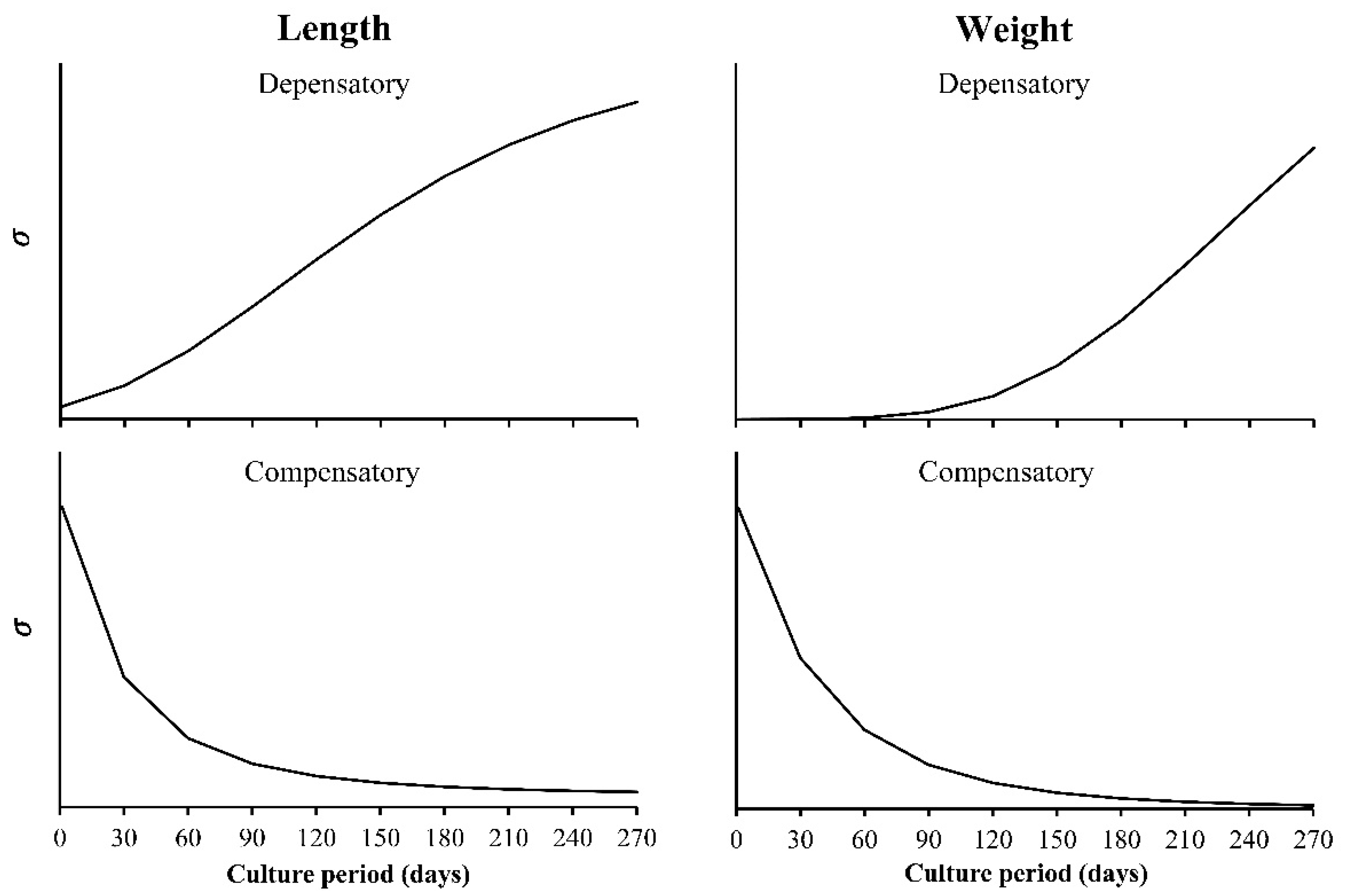
  • Decreasing the variance with x, the independent variable. Here, the included functions are used to simulate the growth compensatory effect [6].
  • The observed variance or age-specific variances. Instead of assuming some type of variances (a, b, or c), the variance obtained from the sample is used, which is estimated from the data. The variance of size at any age (Yo for each value of x), has a square root of σ, which is incorporated into the loglikelihood function. In this case, the lognormal distribution of the residuals is assumed. Then, the sample variance is obtained from the ln(Yo) and not from the original Yo, whereas in the normal distribution, it is calculated from the Yo data for each value of x. For this reason, and despite the importance of the multi-model approach (MMA) or information theory to select models, the focus on variability at age becomes a core strategy in growth analysis.
Growth studies of reared fishes use weight-at-age data more commonly than length-at-age data. Usually, the weight-at-age data describe a sigmoid-shaped growth curve. The growth rate reaches a maximum, which corresponds to the point of inflection in the curve, and then slowly declines to zero when the animals achieve their mature weight. The data in length or weight likely exhibit differences in the standard deviation structure. Therefore, the growth analysis of both datasets becomes important.
Spotted rose snapper (Lutjanus guttatus Steindachner, 1869) farming in floating cages is a novel aquaculture practice in the marine zones of Mexico that yields good income in experimental and commercial stages [9]. The most common growth equations used in reared fishes are the VBGM, the Gompertz growth model, and the logistic model [10,11].
The knowledge of the growth curve is important to improve the production efficiency, including the feeding adjustments. For this reason, the main purpose of this study was to compare the previously used hypothesis of variability at age, assumed as constant, and depensatory and compensatory approaches in growth models against the observed variance proposed in this study. We further aimed to demonstrate the benefit of using the most appropriate standard deviation structure for growth analysis in a dataset of spotted rose snapper cultured in floating cages.

2. Materials and Methods

2.1. Data Source

The data used for this study come from a cultured spotted rose snapper (Lutjanus guttatus Steindachner 1869) farmed for 270 days in marine cages at the eastern coast of the mouth of the Gulf of California. An aleatory sample of 60 fishes was obtained every 4 weeks from the beginning to the end of the trial. The total length (nearest 1 mm) and total weight (nearest 0.1 g) were estimated for each individual (for more detail of culture procedure, see [9]).

2.2. Models and Selection Criterion

After the size-at-age data (length or weight) were obtained, they were plotted to visualize the most suitable growth model that should be applied. In addition, the observed variance from the sample was plotted to visualize the variance criterion. Three asymptotic models were chosen to address the size-at-age data and determine which model was best. An information theory approach was adopted to select the best individual growth model [12,13]. The models were the VBGM, the logistic model, and the Gompertz growth model. The equations are as follows:
The VBGM [14] is given by:
Y t = Y ( 1 e k ( t t 0 ) ) D ,
Logistic [15]
Y t = Y ( 1 + e k ( t t * ) ) 1 ,
Gompertz [16]
Y t = Y e ( e k ( t t * ) ) ,
where Yt is the size at time t, Y is the asymptotic size, t0 is the theoretical age at zero weight or length, t* is the inflexion point of the sigmoid curve and k represents the coefficient of growth. The size is the weight or length in VBGM (in the case of weight, D = 3, and in the case of length, D = 1). Note that using the size as Y, any size can be used, such as the total length, weight, or carapace width, among the other commonly used measured variables.
To estimate the parameters, the objective functions were first suited to consider the following: Y0 is the observed value of the dependent variable, and Ye is the estimated value with any of the candidate models using the likelihood function:
L L = ( 0.5 L N ( σ 2 ) 0.5 L N ( 2 π ) ( Y o Y e ) 2 2 σ 2 ) ,
This function was maximized. To convert the function into negative log likelihood functions, invert the signs (− by +). Using negative likelihood, the objective function is minimized.
The normal distribution of errors was considered (additive error). The sigma (σ) values used according to error residual’s structure criteria were:
Constant:
σ = ( Y o Y e ) 2 n ,
Depensatory:
σ = σ 2 [ ( 1 e k ( t t 0 ) ) D ] 2 ,   for   VBGM
σ = σ 2 [ ( 1 + e k ( t t 1 ) ) 1 ] 2 ,   for   logistic   model
σ = σ 2 [ e ( e k ( t t * ) ) ] 2 ,   for   Gompertz   model
Compensatory:
σ = σ 2 [ ( 1 e k ( t t 0 ) ) D ] 2 ,   for   VBGM
σ = σ 2 [ ( 1 + e k ( t t 1 ) ) 1 ] 2 ,   for   logistic   model
σ = σ 2 [ e ( e k ( t t * ) ) ] 2 ,   for   Gompertz   model
σ 2 is the variance for the oldest organism, similar to L in growth models. That is, σ 2 is the variance at the asymptotic size.
The observed
σ i = ( Y o i Y a i ) 2 n ,
(in this case, the Yoi) is the observed value at each age, and Yai is the average value at each age.
The model criterion selection approach was used to select the best candidate growth model and the best variance criterion based on the Bayesian information criterion (BIC). The BIC was estimated as BIC = 2-LL + ln(n)θi, where LL is the maximum log likelihood, θi is the number of parameters in each model tested plus 1, and n represents the number of observations. The model with the lowest BIC value was chosen as the best model. Differences in the BIC values (Δi = BICi − BICmin) were estimated among the three models used in this study. The BIC weight (Wi) is the percent of evidence in favor of model i. Wi was estimated according to [17] using the following formula:
W i = e ( 0.5 i ) i = 1 3 e ( 0.5 i ) ,

2.3. Confidence Intervals
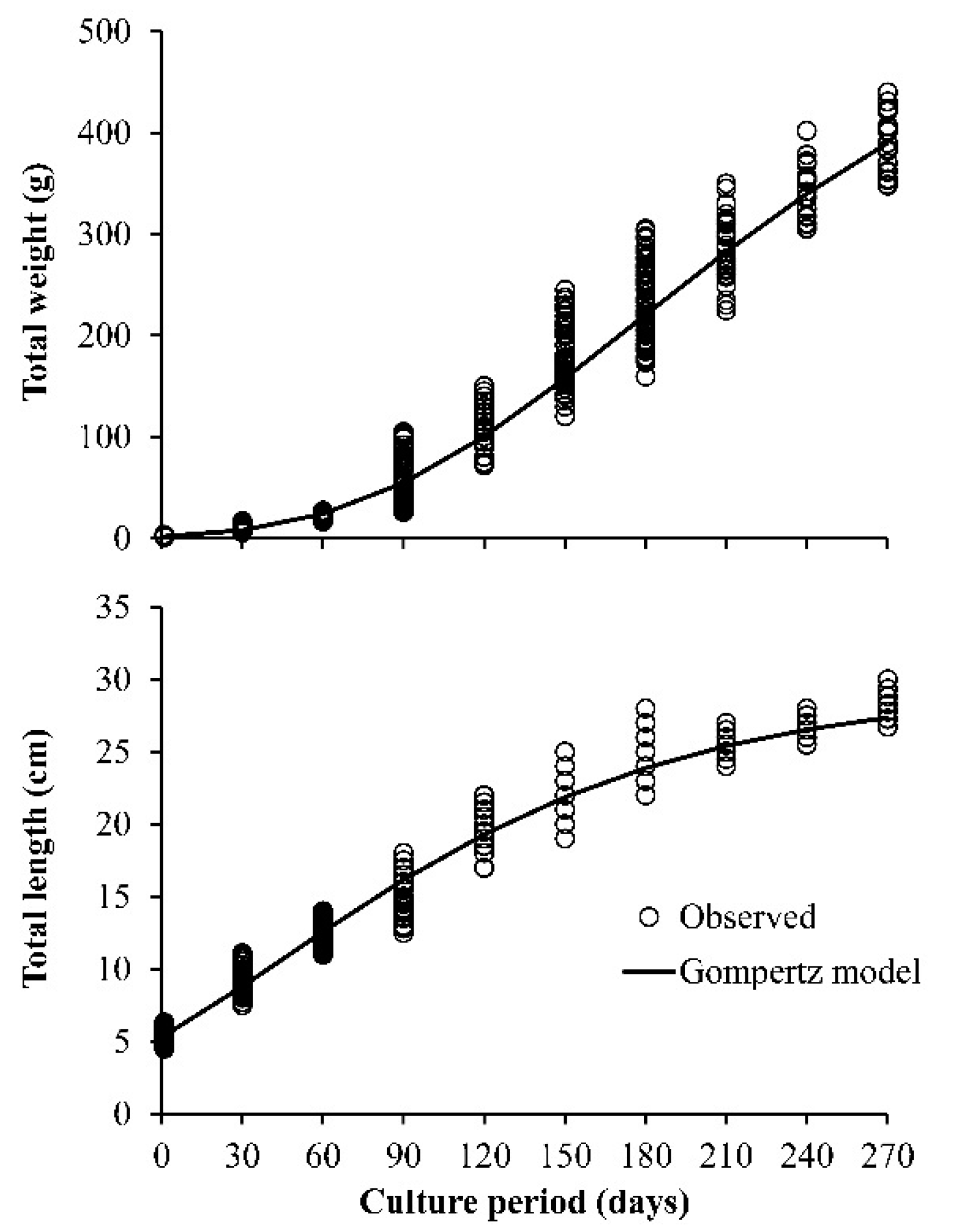
To find a correlation, the joint confidence intervals for L and K were estimated based on likelihood profiles and chi-square distribution [18]. The confidence interval was defined as all values that satisfy the following inequality:
2 ( L ( Y | θ ) L ( Y | θ b e s t ) ) < χ 1 ,   1 2 ,
where L ( Y | θ b e s t ) is the log likelihood of the most likely value of θ, and χ 1 ,   1 2 is the value of X2 with two degrees of freedom at the confidence level of 1-α. Thus, the confidence interval at 95% of the value θ covers all values that are twice the difference between the log likelihood of a θ given and the log likelihood of the best estimate of a θ given one that is less than 5.99.

3. Results

According to observed length data (Figure 1A), the proposed candidate models must be asymptotic because the sizes clearly reached an asymptote around 200 days. The standard deviation was not observed to increase or decrease with the days (Figure 1B). Instead, the standard deviation increased and then decreased. Here, the constant variance should be proposed considering a balance from the beginning and late ages.
In the case of weight, the most likely candidate models should be asymptotic, more likely a sigmoid (Figure 2A). Here, the variability at age is observed to increase with days (Figure 2B), then it was possible to use the criterion of depensatory variance. Obviously, the criterion of compensatory effect does not fit.
Comparing the growth models of the length and weight data with the four variance criteria, it was observed that the lowest BIC was obtained with the Gompertz model using the observed variance (Table 1). The second place was obtained for constant variance in length and depensatory for weight, according to the observed raw data (Table 1).
The trajectories of variance with depensatory and compensatory criterion for length or weight are presented in Figure 3. Adjusted Gompertz growth curves for length and weight are shown in Figure 4. Although the trajectories (length vs. weight) look different, the same model was selected as the best model to describe them.
As the Gompertz model fitted with observed variance was the best model, the parameters for this model and this criteria variance are presented in Table 2. For length, the L did not show a significant difference, even when the depensatory criterion was used. In the weight data, a significant difference was observed among the four criteria. The K value with the observed sigma in length data was only different from that of the compensatory criterion, while in the weight data, the K values were different among the five criteria. The inflection point (t*) was not different from that observed against the other three criteria in the length data, while in the weight data, a significant difference was observed among the four criteria.

4. Discussion

In previous studies of reared fish growth analyses, the constant variance was the criterion used. However, in the present study, the observed variance was the most appropriate to parametrize the three different fitted models. The approach taken in the present study of using the observed variance is novel in fish growth literature. Considering the variability at age, previous analyses have attempted to improve the parametrization of the models [19]. Despite the novelty of the proposed method by reference [19], it has a caveat: it works with constant variance. Other approaches to contrast the constant variance have been tested, including depensatory [7] and compensatory [6] approaches. However, no observed variability at age was tested in reared fishes before this study.
A new challenge in parametrizing growth models is to consider the observed variability at age. The innovation proposed in the present study uses the observed variance instead of using the constant variance. Computing the values of σ i 2 through the optimization of σ 2 led to the best interpretation of the size at age. However, this cannot be observed if the variance is assumed as constant (under the conventional method or unconventional approach). The observed variance has the advantage of demonstrating intrinsic variability of the size at age that cannot be observed if the objective function is solved (as traditionally occurs) based on the conventional constant-variance or the monotonically increasing/decreasing approach.
Considering the variance of the length raw data (Figure 1B) could lead researchers to expect that the model is configured to a constant variance (stable over time). However, it was interesting to observe the differences with respect to the criteria of observed variances. On the other hand, the variance of the weight raw data (Figure 2B) could lead to the use of depensatory variance. Once again, the criteria of the observed variances was the best method to parametrize the models.
Differences in the estimated model parameters were not clearly observed (Table 2) in the length data, while in the weight data, the differences were clear. In other words, relying on the confidence intervals for the model parameters might lead to the conclusion that there the error structure is unimportant because it shows similar growth curves. However, fitting two of the most common size data in the scientific literature of cultured fishes allowed us to show that using the observed variance yields robust results, i.e., in both cases, the observed variance produced the most plausible fits.
Although the objective of the present work was not to select the best model using the MMA but to test differences in the hypothesized variance structure, we found that the Gompertz model using the observed size–age dispersion was the most plausible model. The models chosen at the beginning were coincident with the variance observed as the best technique for parameterization of the models, since the lower value of the BIC was for that criterion in the three models used. It is worth mentioning that, according to the two types of data used (length and weight), it was observed that the variability of the size at each age had a different performance. For the length data, the standard deviation had a distribution that balanced the differences at the beginning and end of the analyzed age period, as mentioned by reference [2]. This enables the analysis of the parameterization of the models using the constant variance criterion, as is also demonstrated by the BIC values that placed it second. In other words, if the observed sigma had not been used, the constant variance criterion would have been the best error structure, indicating the depensatory and compensatory criteria with a negligible percent of evidence in its favor. On the other hand, the weight data have a sigma distribution with a tendency to increase as the age increases (depensatory). The values of the BIC place the depensatory criterion second. Therefore, if the observed variance had not been used, the depensatory criterion would have been the best, the criteria of constant variance would be far away and the compensatory criterion would be farther away. Despite recognizing the variability of sizes at the same age, no criteria should be assumed to plot the dispersion of variance at each age. In our study, we examined the same species growing under the same culture conditions. However, when analyzing two types or sizes (weight and length), each presents a different distribution of size variability at the same age.
We anticipate that this work will introduce a biological structure within a statistical analysis to find biologically important solutions. As mentioned by [20], considering the structure of the standard deviation of length or weight for each age or age classes will result in a better approximation of the growth parameters represented by the collected data. The growth is the result of anabolism (the process of building up body substances) and catabolism. The respiration rate (proportional to anabolism), in turn, is usually proportional to the surface area. Such general principles lead to differential equations for growth processes that are generally applicable to many species, including fishes. A growth equation is any model where weight or length (dependent variable) is calculated using time as the predictor (independent variable). Growth functions are usually analytical solutions to differential equations that can be fit to the growth data. The sigmoidal or curvilinear shape of the growth trajectory indicates that linear regression is not suitable to describe growth unless only small portions of the curve are considered. For this reason, nonlinear growth functions are the best means of estimating the growth of fishes. For a long time, fish growth under culture conditions has been described by increasing weight over the culture period. Recently, researchers [10,11] have shown that the growth-fitted model is a more informative way to describe the growth patterns of cultivated fish. A model fitted to the specific culture conditions allows accurate interpolation of the weight at any time in the observation range and not just when the data were obtained. Interpolations or extrapolations are not possible without fitting a model. If an aquaculturist knows the anticipated growth curve of a species under reared conditions, they can adjust the feeding regime. Feed is the most important expense in industrial aquaculture, so the estimation of appropriate growth parameters will improve culture management.

5. Conclusions

Using the observed variance in the present study was the best method to parametrize the three commonly used individual growth models (von Betalanffy, logistic, and Gompertz) using size-at-age data (length weight) for cultured fishes. In particular, this study used the spotted rose snapper as a study case. The information criterion indicated that the observed standard deviation yielded the most plausible models. We therefore conclude that, whenever possible, the observed error structure should be used to conduct robust estimates of individual growth parameters.

Author Contributions

Data curation, E.A.A.-N.; formal analysis, S.G.C.-V., E.A.A.-N. and G.R.-D.; investigation, S.G.C.-V. and E.A.A.-N.; methodology, S.G.C.-V., E.A.A.-N. and G.R.-D.; supervision, E.A.A.-N.; writing—review and editing, L.M.-C., E.A.-M. and Á.J.B.A. All authors have read and agreed to the published version of the manuscript.

Funding

This research received no external funding.

Institutional Review Board Statement

The authors followed the international and national code to preserve the wellbeing of animals under investigation.

Informed Consent Statement

Not applicable.

Acknowledgments

We are indebted to the Santiago Rocha from “Laboratorio Acuicola ALAPSA” and Bernardo Quintero for access to spotted rose snapper growth data. We also thank Edgar Alcántara from CIBNOR-Guaymas Applied Ecology and Fisheries lab for improving the figures.

Conflicts of Interest

The authors declare no conflict of interest.

References

  1. Beverton, R.J.H.; Holt, S.J. On the Dynamics of Exploited Fish Populations; Ministry of Agriculture, Fisheries and Food; Fisheries Investigations: London, UK, 1957. [Google Scholar]
  2. Schnute, J.; Fournier, D. A New Approach to Length–Frequency Analysis: Growth Structure. Can. J. Fish. Aquat. Sci. 1980, 37, 1337–1351. [Google Scholar] [CrossRef]
  3. Sainsbury, K.J. Effect of Individual Variability on the von Bertalanffy Growth Equation. Can. J. Fish. Aquat. Sci. 1980, 37, 241–247. [Google Scholar] [CrossRef]
  4. Letcher, B.H.; Coombs, J.A.; Nislow, K.H. Maintenance of phenotypic variation: Repeatability, heritability and size-dependent processes in a wild brook trout population. Evol. Appl. 2011, 4, 602–615. [Google Scholar] [CrossRef] [PubMed]
  5. Luquin-Covarrubias, M.A.; Morales-Bojórquez, E.; González-Peláez, S.S.; Hidalgo-De-La-Toba, J.Á.; Lluch-Cota, D.B. Modeling of Growth Depensation of Geoduck Clam Panopea globosa Based on a Multimodel Inference Approach. J. Shellfish. Res. 2016, 35, 379–387. [Google Scholar] [CrossRef]
  6. Félix-Ortiz, J.A.; Aragón-Noriega, E.A.; Castañeda-Lomas, N.; Rodríguez-Domínguez, G.; Valenzuela-Quiñónez, W.; Castillo-Vargasmachuca, S. Individual growth analysis of the Pacific yellowlegs shrimp Penaeus californiensis via multi-criteria approach. Lat. Am. J. Aquat. Res. 2020, 48, 768–778. [Google Scholar] [CrossRef]
  7. Restrepo, V.R.; Diaz, G.A.; Walter, J.F.; Neilson, J.D.; Campana, S.E.; Secor, D.; Wingate, R.L. Updated estimate of the growth curve of Western Atlantic bluefin tuna. Aquat. Living Resour. 2010, 23, 335–342. [Google Scholar] [CrossRef] [Green Version]
  8. Aragón-Noriega, E.A.; Mendivil-Mendoza, J.E.; Alcántara-Razo, E.; Valenzuela-Quiñónez, W.; Félix-Ortiz, J.A. Multi-criteria approach to estimate the growth curve in the marine shrimp, Penaeus vannamei Boone, 1931 (Decapoda, Penaeidae). Crustaceana 2017, 90, 1517–1531. [Google Scholar] [CrossRef]
  9. Castillo-Vargasmachuca, S.G.; Ponce-Palafox, J.T.; Muñoz, E.A.; Rodríguez-Domínguez, G.; Aragón-Noriega, E.A. The spotted rose snapper (Lutjanus guttatus Steindachner 1869) farmed in marine cages: Review of growth models. Rev. Aquac. 2016, 10, 376–384. [Google Scholar] [CrossRef]
  10. Baer, A.; Schulz, C.; Traulsen, I.; Krieter, J. Analysing the growth of turbot (Psetta maxima) in a commercial recirculation system with the use of three different growth models. Aquac. Int. 2010, 19, 497–511. [Google Scholar] [CrossRef]
  11. Ansah, Y.B.; Frimpong, E.A. Using Model-Based Inference to Select a Predictive Growth Curve for Farmed Tilapia. N. Am. J. Aquac. 2015, 77, 281–288. [Google Scholar] [CrossRef]
  12. Katsanevakis, S. Modelling fish growth: Model selection, multi-model inference and model selection uncertainty. Fish. Res. 2006, 81, 229–235. [Google Scholar] [CrossRef]
  13. Katsanevakis, S.; Maravelias, C.D. Modelling fish growth: Multi-model inference as a better alternative to a priori using von Bertalanffy equation. Fish Fish. 2008, 9, 178–187. [Google Scholar] [CrossRef]
  14. Von Bertalanffy, L. A quantitative theory of organic growth. Hum. Biol. 1938, 10, 181–213. [Google Scholar]
  15. Ricker, W.E. Growth rates and models. In Fish Physiology. Bioenergetics and Growth; Hoar, W.S., Randall, D.J., Brett, J.R., Eds.; Academic Press: London, UK, 1979; pp. 677–744. [Google Scholar]
  16. Gompertz, B. On the nature of the function expressive of the law of human mortality, and on a new mode of determining the value of life contingencies. Philos. Trans. R. Soc. Lond. 1825, 115, 513–583. [Google Scholar] [CrossRef]
  17. Burnham, K.P.; Anderson, D.R. Model Selection and Multimodel Inference: A Practical Information-Theoretic Approach; Springer: New York, NY, USA, 2002. [Google Scholar]
  18. Venzon, D.J.; Moolgavkar, S.H. A Method for Computing Profile-Likelihood-Based Confidence Intervals. Appl. Stat. 1988, 37, 87. [Google Scholar] [CrossRef]
  19. Chen, Y.; Fournier, D. Impacts of atypical data on Bayesian inference and robust Bayesian approach in fisheries. Can. J. Fish. Aquat. Sci. 1999, 56, 1525–1533. [Google Scholar] [CrossRef]
  20. Curiel-Bernal, M.V.; Aragón-Noriega, E.A.; Cisneros-Mata, M.Á.; Sánchez-Velasco, L.; Jiménez-Rosenberg, S.P.A.; Parés-Sierra, A. Using Observed Residual Error Structure Yields the Best Estimates of Individual Growth Parameters. Fishes 2021, 6, 35. [Google Scholar] [CrossRef]
Figure 1. Row length data. (A) Length at age and (B) observed variability at age (solid line) and tendency (dashed line).
Fishes 06 00060 g001
Figure 2. Row weight data. (A) Weight at age and (B) observed variability at age (solid line) and tendency (dashed line).
Fishes 06 00060 g002
Figure 3. Standard deviation (sigma) curves.
Fishes 06 00060 g003
Figure 4. Growth curves of the Gompertz model fitted with the observed variance.
Fishes 06 00060 g004
Table 1. The Bayesian information criterion (BIC) for each of the three models and the four residual structures.
VariableResidual StructureVBGMLogisticGompertz
LengthObserved171117711668
Constant185218291811
Depensatory267319471867
Compensatory300120112022
WeightObserved441146954403
Constant512751995199
Depensatory467448544669
Compensatory5953117685939
Table 2. Parameters and 95% confidence intervals (CI) for the Gompertz model with different residual error structures. L is the asymptotic length, W is the asymptotic weight, t* is the inflexion point of the sigmoid curve, and k represents the coefficient of growth.
Length Weight
CriterionOptimum (CI)SignificanceOptimum (CI)Significance
L (cm) W (g)
Observed29.44 (29.25–29.64)a578 (570–586)a
Constant29.79 (29.44–30.19)ab403 (398–409)b
Depensatory29.23 (28.99–29.47)a507 (493–521)c
Compensatory30.25 (29.64–30.94)b1738 (1707–1776)d
k (days−1) k (days−1)
Observed0.01168 (0.01143–0.01194)a0.00993 (0.00988–0.00999)a
Constant0.01138 (0.01090–0.01188)ab0.02320 (0.02240–0.02420)b
Depensatory0.01179 (0.01154–0.01204)a0.01054 (0.01046–0.01061)c
Compensatory0.01056 (0.00980–0.01133)b0.00340 (0.00329–0.00341)d
t* (days) t* (days)
Observed46.2 (45.5–46.9)ab176.3 (175.8–176.9)a
Constant47.3 (46.2–48.3)a165.3 (163.9–166.7)b
Depensatory45.0 (44.4–45.7)ab161.6 (161.0–162.2)c
Compensatory44.8 (43.4–46.2)ab386.2 (384.7–387.7)d
Publisher’s Note: MDPI stays neutral with regard to jurisdictional claims in published maps and institutional affiliations.

