1. Introduction
Magnetic field measurements can be performed with a variety of sensors characterized by very broad ranges in terms of sensitivity, robustness, dynamicity, linearity, reliability, speed, simplicity, and cost. The state-of-art sensors in terms of sensitivity are based on the superconductor quantum interference devices (SQUIDs), which surpass the sensitivity level of
. The main drawback of SQUIDs is their need for cryogenics. Optical atomic magnetometry constitutes another technology that in some implementations—particularly in the so-called Spin-Exchange-Relaxation-Free (SERF)—may compete with SQUIDs in terms of sensitivity. It also enables the construction of relatively simple and robust sensors with sensitivity at the
level and below, including miniaturized devices, and implementations with a high-frequency response. Optical atomic magnetometers (OAMs) do not require cryogenics. On the other hand, they are commonly based on spectroscopy in high quality vapor cells illuminated with laser sources, both features that render them expensive and not easily integrable in solid state devices. When these extreme performances are not required, fluxgate technology offers an eligible alternative, on the basis of which different grades of sensors are produced with a rather wide range of sensitivities and costs. When sensitivities of the order of
are sufficient, beside the low-cost fluxgate sensors, solid-state technology now offers extremely cheap and easy-to-use devices based on the magnetoresistive effects. The magnetoresistive effect (discovered and first studied by Lord Kelvin [
1,
2]) in its giant [
3], tunnel [
4], and anisotropic [
5] occurrences, can be profitably used to measure fields of several tens of micro Tesla, that is, of the order of the geomagnetic field, with typical sensitivities in the
range and bandwidth extending up to kHz, or—depending on the implementation—to MHz and beyond [
6]. Devices based on magneto-resistance (MR) with sensitivity levels attaining
above 1 kHz have been reported [
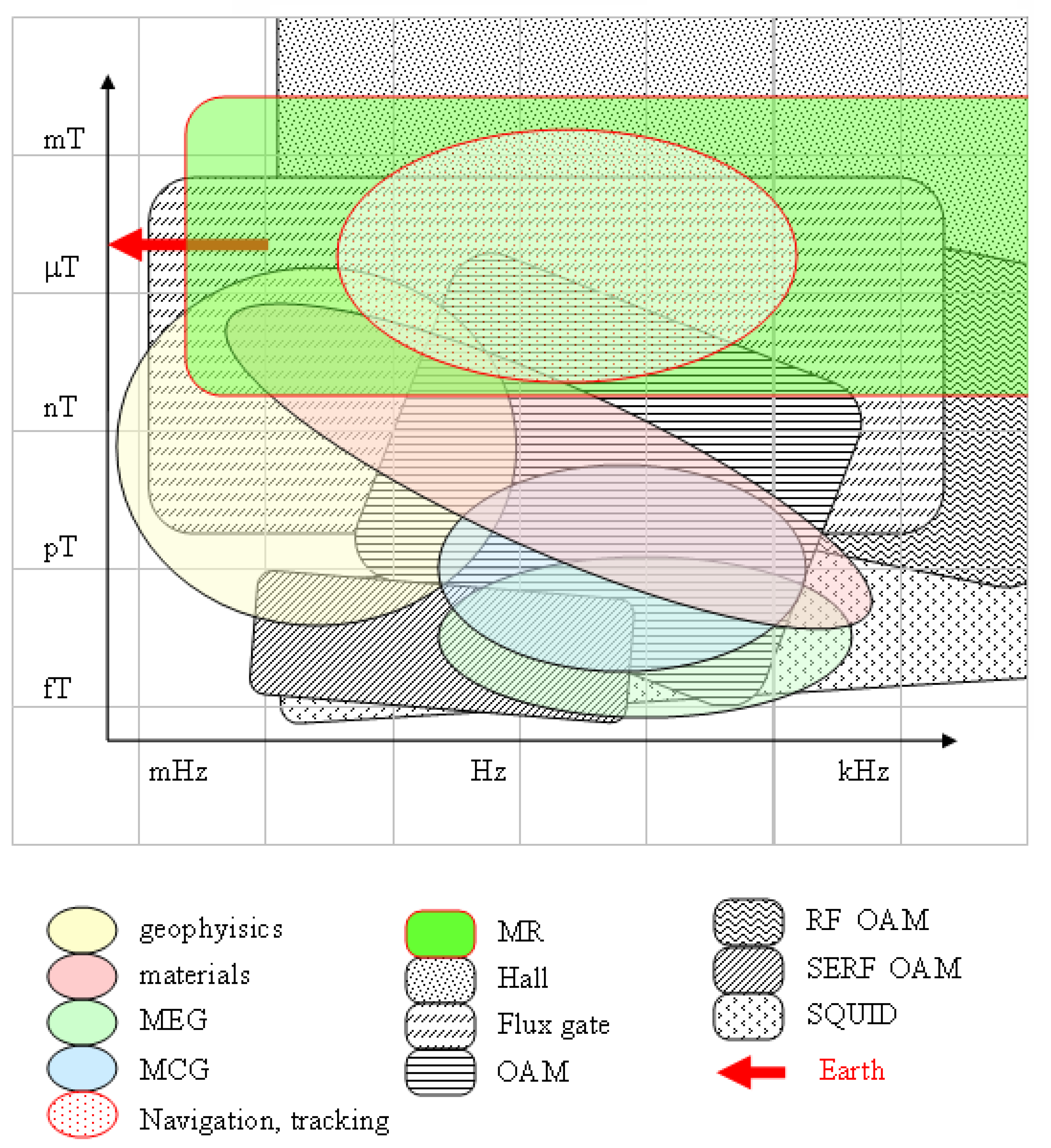
7]. The magnetoresistive sensors (similarly to SQUIDs and fluxgates, and in contrast to typical OAM magnetometers) are vectorial in nature, that is, respond to single components of the magnetic field: an assembly of three orthogonally oriented sensors enables complete measurement of the magnetic field vector. Other popular solid state sensors are based on the Hall effect: their sensitivity and accuracy is worse than MR and they are more commonly used to roughly estimate (or rather just to detect) relatively strong fields. A synthetic, rough overview of the technologies available and of the accessible bandwidth and sensitivity intervals for magnetometric measurements is provided in
Figure 1.
The success of MR technology is also related to its easy integration with silicon-based electronic devices. Integrated circuits (ICs) containing one or more magnetoresistive elements have recently become very popular, and their cost has decreased by orders of magnitude over the last decade, thanks to large-scale production: nowadays two- or three-axis devices are widely used as sensors for electronic compasses, such as those contained in smartphones and drones. Other applications for these cheap sensors include virtual and augmented realities, navigation, non-destructive evaluation, and various industrial activities [
6,
8,
9]. Modern MR ICs contain not only magnetoresistive sensors but also signal conditioning and DAQ electronics, together with special reset circuits that facilitate the MR use and improve reliability and reproducibility of their response, as well as circuitry for digital data transfer.
We focused our attention on a family of ICs designed for Inter-Integrated-Circuit (I2C) protocol transmission of 3D magnetic data, which allows for an acquisition and data transfer rate as fast as 200 readings (3 data per read) per second. Due to the typical presence of a single sensor per user, in most cases these ICs have a static (not re-configurable) I2C address. Some devices do, however, have a re-configurable address. In the case of the IC used in our prototypes, two address configuration pins (for a maximum of four chips per bus) are available. This limitation leads us to develop control-interface circuits with a parallelized architecture, when a sensor array is needed. At the cost of the obviously heavier circuitry, such an approach brings the second (but not secondary) advantage of accelerating the data acquisition and making it simultaneous throughout the sensor set.
The aim of our work is to acquire, at a relatively high rate (hundreds of samples per second), magnetometric data sets that can be elaborated to reconstruct the position of magnetic field sources, that is, to track their spatial co-ordinates and the angles of their orientation. In the frequent case of a simple source like a magnetic dipole [
10,
11,
12], the tracking procedure provides three spatial coordinates and three components of the magnetic dipole. As soon as the measurement is performed in an external field (such as the geomagnetic field, which can be assumed homogeneous over the volume of the sensor frame), three more field components have to be worked out, making a total of
tracking data to be extracted per measurement. These 9 data contain redundant information in the case of repeated measurements, because both the modulus of the dipole moment and the modulus of the ambient field can be assumed to be constant. This means that rotations of the dipole around its direction and rotations of the sensors around the ambient field do not cause field variations: these rotations correspond to
blind co-ordinates. In other terms, if it can be assumed that the intensity of the magnetic source and/or of the environmental field are constant, the number of freedom degrees (and hence of the fitting parameters) would be reduced from 9 down to 8 or 7.
The information about the two blind co-ordinates could be retrieved using a non-dipolar source (e.g., a set of two rigidly connected dipoles) and by complementing the environmental magnetic field with a measurement of the gravitational field. We will not address these possible improvements in this paper. The use of non punctual sources, with the introduction of multipolar terms that break the dipole symmetry, has been successfully attempted and reported in the literature [
13].
Similarly, the system could be used to track two or more dipolar sources, located arbitrarily with respect to each other [
14,
15]. In this case, the enhancement in the source’s degrees of freedom would require more computing resources and an increase of the minimum number of sensors.
The ability to track objects with an adequately fast time response is a challenging and intriguing achievement, with important implications in several areas of research and applications. In particular, tracking methods based on magnetometric measurements offer a minimally invasive methodology and have been studied/proposed in a variety of applications, including medical diagnostics [
16], the tracking of vehicles [
17], biology [
18], and robotics [
19].
Further possible applications may arise in other diverse areas, also depending on the precision and the speed that can be achieved, such as body part tracking (eye, tongue, hand, finger), human-computer interfaces, virtual and augmented reality, and so forth.
Several approaches have been proposed to deal with the inverse problem of reconstructing the field source parameters from the field measurement (see e.g., Reference [
20] and references therein). Depending on the application, the requirements in terms of accuracy, precision, robustness and speed of the tracking procedure may change, and different methodologies can be applied.
2. Setup Overview
We have designed and built an interface circuit capable of operating arrays made of up to eight three-axis MR sensors, which can be differently disposed and grouped within the space.
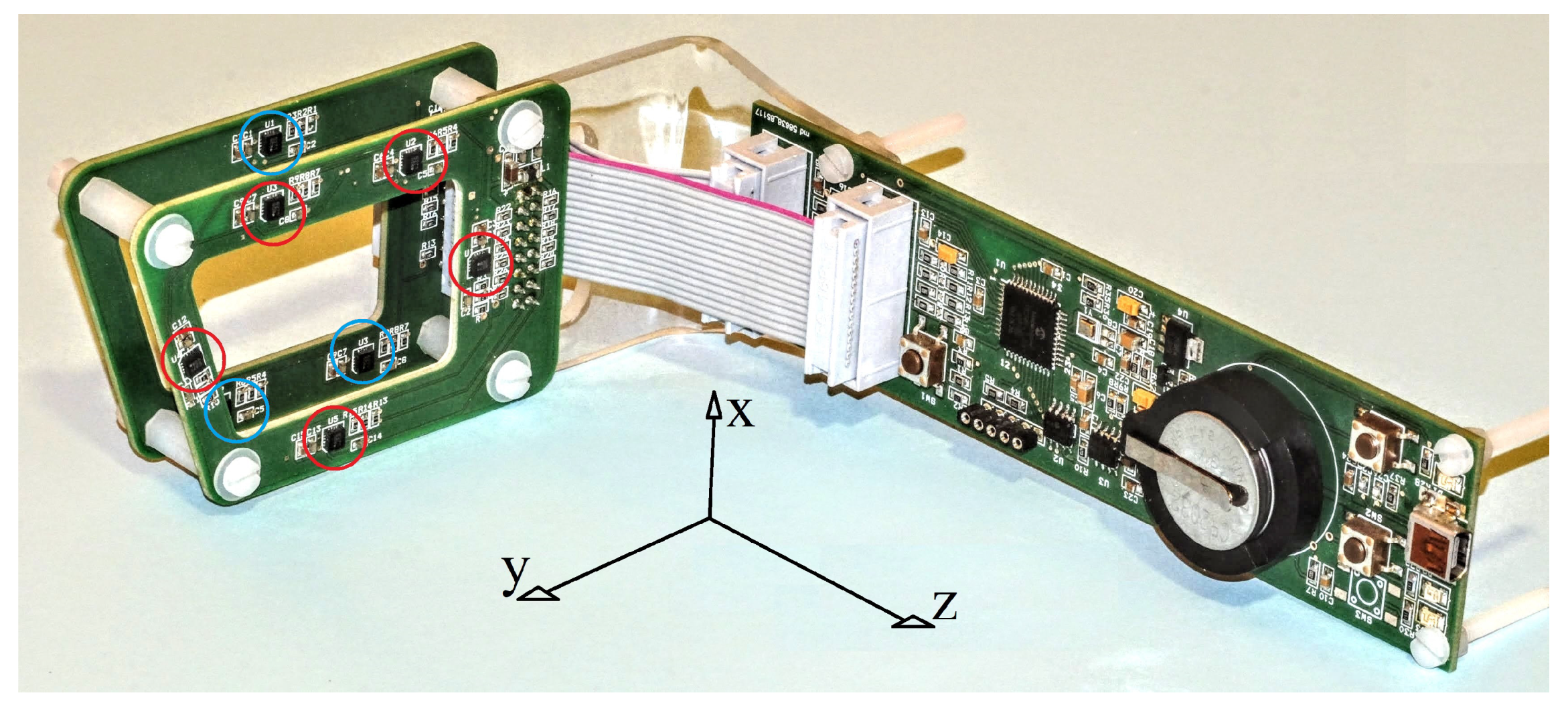
A picture of a sensor array and related interface electronics is shown in
Figure 2. A printed circuit board (PCB) hosting a micro-controller, Electrically Erasable Programmable Read-Only Memory (EEPROM), internal and external supply circuitry and a USB interface is connected to two sensor-PCBs, which can host 4 + 4 or 5 + 3 IC sensors (as shown in that
Figure 2). Each sensor has a dedicated I
2C bus for communicating with the micro-controller. The limited number of address-bits available makes some degree of parallelization necessary. We opted for a fully parallel architecture (one I
2C bus for each IC) that –at the expense of a slightly heavier circuitry—brings several advantages, among which—simultaneous measurements; simpler firmware; and no need to transmit data over the bus along the conversion (this avoiding a possible source of noise). Hence the microcontroller may send commands (and receive data) simultaneously to (and from) the eight sensors. The data can be either immediately transmitted to the computer or stored on an EEPROM for subsequent download. The second option is used when acquiring data for the calibration procedure (see
Section 5 below). Details of the functionalities available and consequent possible operations are provided in the next sections. These are designed in view of producing fast (real time) tracking devices with a high throughput rate (100 trackings per second in the current implementation) and precision (sub-millimetric spatial- and 2 degree angular-resolution).
3. Sensor Specifications
The Isentek IST8308 IC [
21] is a three-axis magnetometer based on the anisotropic magnetoresistance effect, whose main characteristics are reported in
Table 1. The chip implements reset, temperature compensation and analogue-to-digital conversion circuitry, and communicates trough an I
2C port. Both on-demand and continuous data outputs can be queried. The maximum data acquisition rate is 200 Sa/s, and different kinds of internal filters can be activated to improve the signal-to-noise ratio at the expense of the effective bandwidth. Sensitivity and offset have non-negligible deviations from ideality (zero offset and maximum count at full-scale field), so that a calibration is necessary (see
Section 5). These parameters may also change with time and (slightly) with temperature, so that an adequate measurement accuracy can be maintained at the cost of repeated calibrations. It is worth noting that the temperature compensation circuitry helps reduce this problem, since the effects of typical daily environmental temperature drifts can be neglected. In our implementation, a temperature sensor has been included, so that the user knows both the temperature at which the calibration data were collected and the current temperature: when the deviation exceeds a threshold level, an alert is provided, making renewed calibration advisable. A data-consistency analysis is also available in order to highlight the need to re-calibrate the unit, as discussed at the end of
Section 5.
4. Scalability
The system developed aims to simultaneously measure the environmental field and the field generated by a small, closely located magnetic source (dipolar magnet). The finite dynamic range of the sensors makes it necessary to deal with field contributions of comparable intensities. This condition should be fulfilled at least on a sensor subset providing a number of independent data sufficient to localize the magnet, that is, not smaller than the number of freedom degrees of the system.
Good operating conditions can be identified as those in which the dipole generates fields on the sensors ranging from 1/10 to 10 times the ambient one. Thus, keeping in mind the typical environmental field value of some tens of T, the dependence of the dipolar field, and the magnetization values of permanent magnets (about 1T/ for the neodymium devices used), one finds that the best condition is fulfilled when the sensor-magnet distance is about 50 times larger than the linear size of the magnet. For example, a one cm3 magnet produces a field comparable to the Earth’s field at about a half-meter distance. The chip size being sub-millimetric, this rule of thumb applies when scaling down the system size as long as the sensor-magnet distance remains much larger than the sensor size (e.g., magnets as small as 1 mm in size can be used at a distance of about 5 cm from the sensors).
Of course, according to the tracking accuracy required, the sensor positions must be known with an adequate level of precision. In our case, the latter is determined by the PCB mount and is sub-millimetric. However, determination of the sensor positions can be improved on the basis of magnetometric data analysis [
22], and in some of our preliminary prototypes this kind of procedure was found to be crucial to guaranteeing the reliability of the tracking algorithms.
5. Sensor Calibration
MR sensors have a relatively accurate response in terms of linearity, but suffer from significant offset and variable gain. Moreover, both gain and offset may vary with changes in temperature and in time. In addition, unpredictable values are found after powering up the device.
An important improvement has been introduced on the basis of a pulsed field-cycling technique. This reset field pulse technique has also been studied to improve the ultra-low frequency performance of MR devices [
23]. Modern magnetoresistance ICs contain apposite inputs to apply reset pulses (strong current pulses flow into a conductor built in the proximity of the magnetoresistive element, in order to re-magnetize its components in an appropriate and reproducible way).
In more integrated devices the current pulses are produced internally and the reset field cycle is automatically applied at the restart. The reset operation leads the sensor to work properly (reasonably low offsets and reasonably ideal gains along all the axes); nonetheless whenever good accuracy is required, some sort of calibration procedure [
24] is advisable or necessary. In fact, the final offset value is substantially non-zero, and the gain may differ by several percent among the sensors contained in a single IC. An accurate evaluation of the offsets and gains makes it possible to convert the raw data into field measurements, so as to overcome these non-idealities.
Our setup includes apposite parts devoted to facilitate the calibration procedure in the hardware, firmware, and software. Similarly to what is described in Reference [
24], the calibration procedure is accomplished by recording many data (simultaneously for all the 3D sensors of the array), while rotating the system freely and randomly in a (nominally) homogeneous field. In this measurement, each sensor detects the magnetic field vector
as it moves on a spherical surface centered in the zero-field point of a Cartesian co-ordinate system: whenever the quantities
do not span a spherical surface, this can be due to non-zero offsets, to unequal gains, and to non-linear terms in the sensors’ response. In the hypothesis of a linear response, the quantities measured describe an off-center ellipsoid rather than a centered spherical surface: the displacement of the center is caused by the offsets, while the eccentricity is due to the gain anisotropy.
It is worth noting that literature reports similar calibration procedures based on static measurements [
25]. It is indeed possible to build a tri-axial field generator, finely calibrate it with the help of a scalar magnetometer and then use it to produce a rotating field of an assigned intensity. The latter can, in turn, be applied to calibrate vectorial sensors such as tri-axial magnetoresistive devices.
An optimization procedure is used to determine offsets and gains for all the sensors, and to save those values for subsequent data conversion. As described below (see
Section 6), this kind of calibration measurement is more favorably performed with no cable connection. The optimization is usually done over data sets containing several hundreds of measurements (a maximum of N = 2000 measurements is set by the EEPROM size), with the minimized quantity being
where
are the raw data; the indexes
both run from 1 to 3 and denote the three Cartesian components;
k is the sensor index running from 0 to
,
are the offset vectors to be determined;
are elements of triangular matrices (to be determined);
n denotes the measurement index (running from 1 to N); and
is the ambient field modulus. The latter can be assigned arbitrarily, or from an independent measurement performed by scalar sensor (e.g., an atomic magnetometer) if quantitative field and dipole-moment estimations are required.
The elements are ideally equal for (the inverse gains), while the off-diagonal elements are ideally zero for . In contrast, the diagonal elements can be different from each other if the gain is not isotropic, and the off-diagonal elements could be non-zero, in the case of possible small misalignments (imperfect orthogonality) of the three axes.
Let the optimal offsets and conversion matrices be given by
and
, respectively, and let’s define
that is, the
ith component of the field in the position
of the
kth sensor, as obtained from the sensor’s output
in the
nth measurement.
Once the offsets are removed and the response has been made isotropic, further calibration is necessary to refer all the sensors to one co-ordinate system. To this end, the data recorded in the calibration measurement mentioned are compared to each other. One sensor (let it be the 0th one) is selected as a reference one, and a rotation matrix is determined for each sensor with
…
by minimizing the vector differences between the field measured by that sensor and the reference one. In our implementation the rotation matrices are defined in terms of Euler angles, and the minimized quantities are:
where
are rotation matrices defined by the three angles
to be determined for each
…
.
In conclusion, each of the K sensors requires the determination of nine parameters (three offsets, three gains, three orthogonality-imperfection-compensation terms) for the conversion of the recorded values into magnetic induction vectors and each sensor (apart from the reference one) requires the determination of three rotation angles. The whole set of calibration parameters ( in the case considered, of sensors) is saved at the end of a calibration procedure and made available to perform the conversions in the subsequent measurements.
Both the minimizations of
f (Equation (
1)) and
g (Equation (
3)) are not critical in terms of convergence, and the calibration result is systematically reliable. Different algorithms can be used in order to execute the two tasks. In the current software implementation we are using the simplex (Nelder Mead) [
26] routine, which is available among the Labview libraries.
Once the calibration parameters have been determined, a field estimation referenced to a unique Cartesian frame is available. This enables an additional procedure to check the validity persistence of the calibration parameters. This validation is performed by comparing the field components measured by the
K sensors in the homogeneous field with their median value. In particular, for each sensor, the software evaluates the quantity
where
denotes the
ith component of the field as measured by the
kth sensor at the
nth measurement in a set of
N, and
denotes the median value of the
ith component of the field measured by the
K sensors at the
nth measurement. The presence of anomalously large
values produces an alert, and the user can disregard the data from the corresponding sensor(s) in the subsequent tracking, or decide to perform a new calibration.
6. Power Supply
The circuit is normally supplied through the USB port, however it is possible to start it in a battery-supply mode, in order to acquire and store the calibration data with no cable constraints. To this end, there is a button to connect the battery, and a button to start the calibration measurement. When the calibration measurement starts, a circuit maintains the battery connection. During this self-supplied operation, a flashing LED denotes acquisition. At the end of the acquisition, the self-supplied mode is maintained for a 30 s, during which the operator can connect the cable. In this manner, the circuit remains supplied, and no reset pulses are applied. This feature is designed to guarantee that the data acquired accurately describe the sensor response, since the latter could be modified in the case of an IC reboot, due to the automatically applied reset pulses.
7. Parallel I2C Buses
Apart from the above mentioned problem arising from the fixed I2C address (a feature that characterizes many types of MR ICs), it is advantageous to parallelize the communication with sets of ICs, both to accelerate the global data acquisition rate and to enable simultaneous (i.e., mutually time-consistent) measurements. We have studied and developed a simple but effective circuit, enabling both parallel data reading from the sensors and fast composite data transmission to a PC. The electronics developed may communicate (for hardware configuration and data transfer purposes) with eight () chips at once, thus providing up to magnetometric data per reading. The data transfer rate is limited either by the sensor throughput rate over the I2C bus or by the composite data transmission rate over the USB port: in the present implementation a rate as high as 100 Sa/s (2400 data/s) has been demonstrated, while 200 Sa/s (4800 data/s) is the limit set by the IC specifications. Concerning the USB communication, this represents a potential bottle-neck. Its speed is machine-dependent and may vary unpredictably for example, with the number of processes running in the computer, and particularly with the presence of other connected interfaces.
8. Firmware
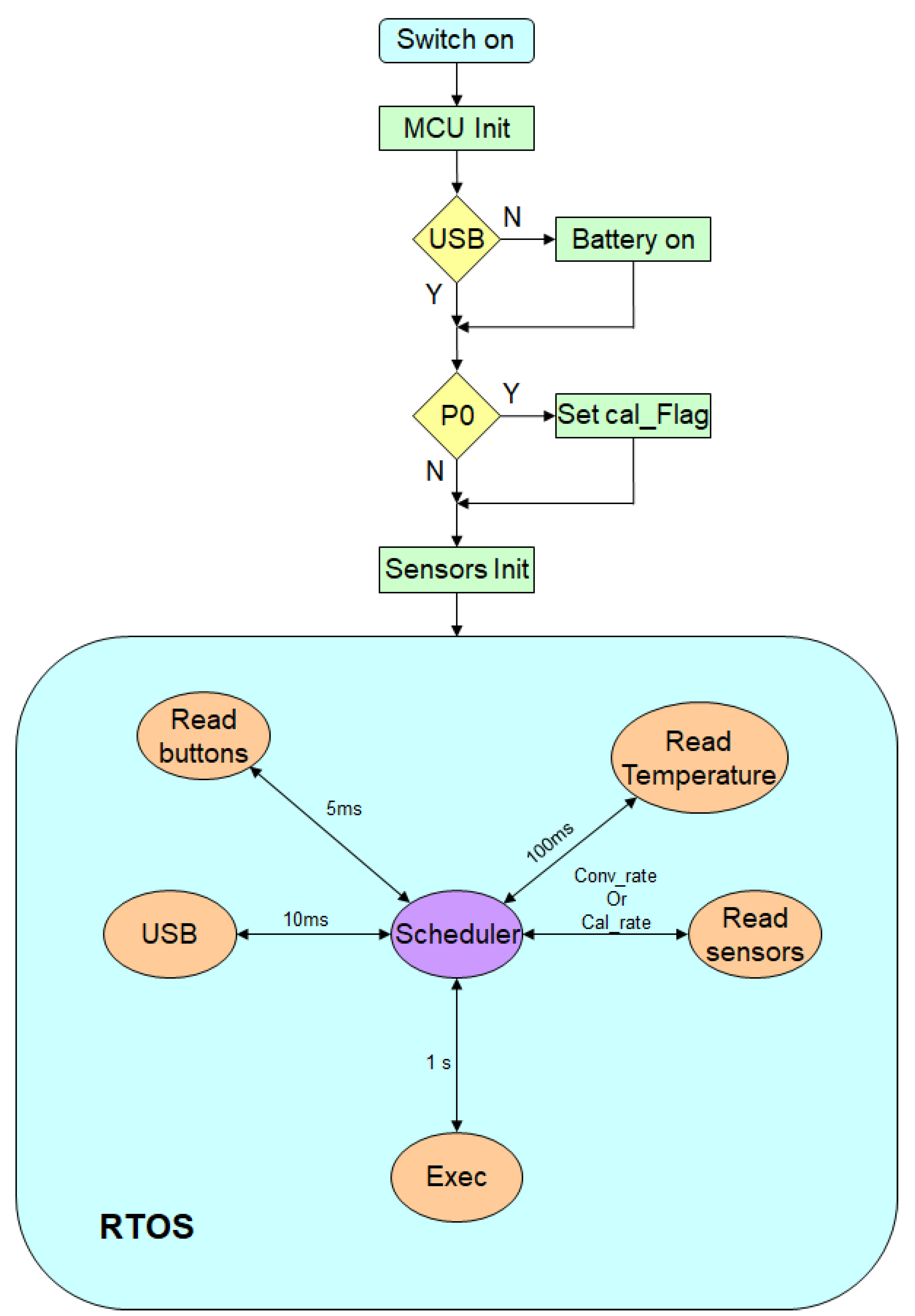
An overview of the firmware principle of operation is represented in
Figure 3. When the system starts up, the peripherals of the microcontroller are configured and the variables used (MCU Init) are initialized. In particular, among the peripherals configured, it is worth mentioning the ADC converter which measures the supply voltage and the timer for the real time operating system (RTOS) described below. In addition, a map is built of the sensors that are actually connected. The latter is then used when the data are transferred from the parallel I
2C buses to the on-board memory or to the USB interface, as described in
Section 7.
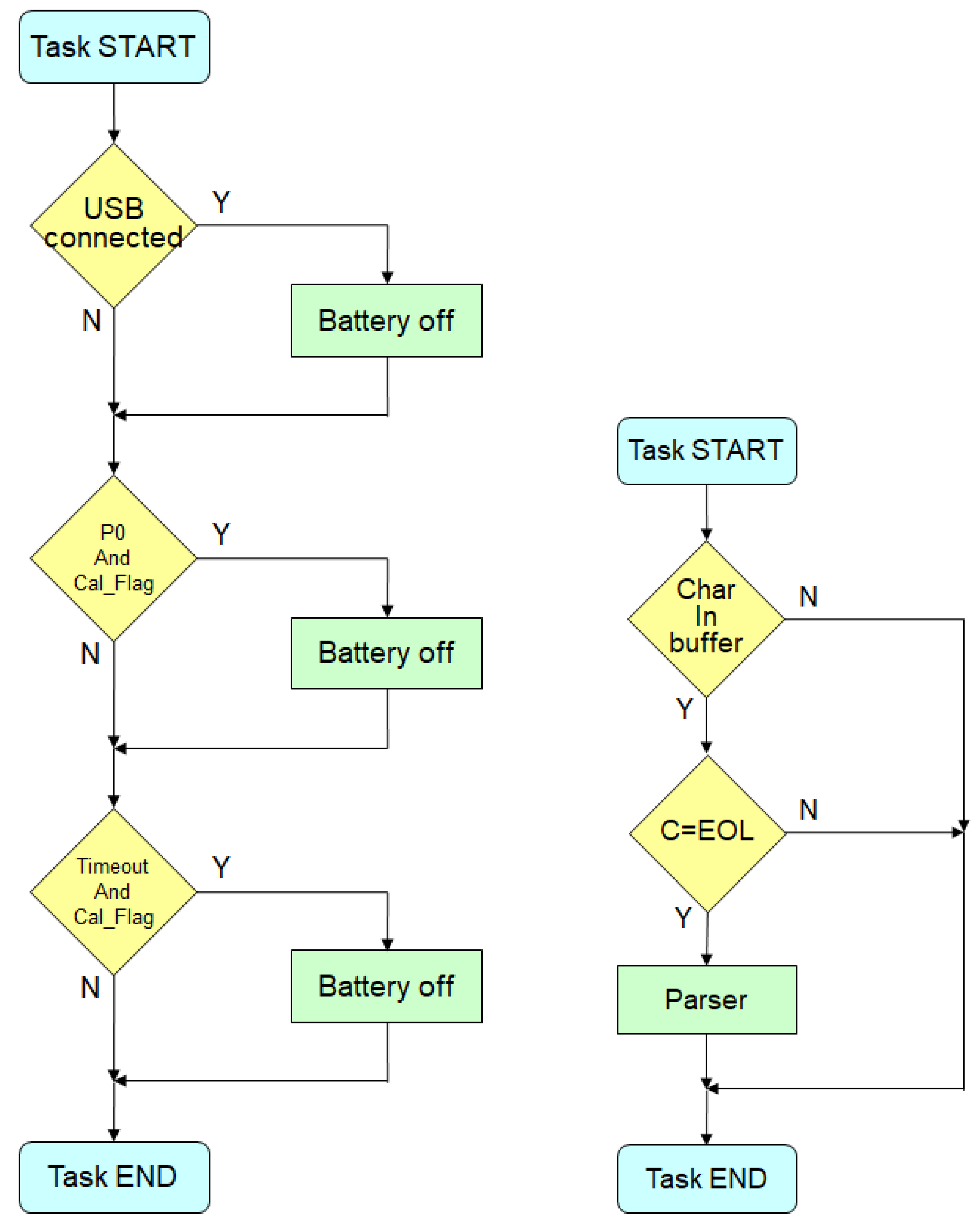
Subsequently, a test is performed to verify whether the system has been started by connecting the USB cable or by pressing the power button: in the second case a switch (MOSFET transistor) is closed, in order to maintain the battery power supply when the power button is released by the user.
At the same time, whether or not the system calibration button (P0) was also pressed during the power-up phase it is also evaluated; in this case a flag variable called cal_Flag is set to True. This flag is used during the operation of the RTOS. The next operation (Sensor Init) is the initialization of the sensors that have been detected and included in the sensor map.
Now the RTOS can start. A scheduler establishes the execution sequence and times of the various programs (tasks) within an iterated cycle. During this cycle the scheduler evaluates –for each task– whether it is time to run it, on the basis of the time elapsed after the last execution: individual time intervals are defined for each task.
The tasks to be performed are:
Reading the state of the buttons (Read buttons) (every 5 ms)
Granting communication between the module and the PC via a USB interface (USB) (every 10 ms). If the buffer contains a character, this is added at the end of a string variable. If this character is a line termination character, the string variable is analyzed by a subroutine (Parser) and, if it is recognized as a valid command, such command is executed.
Performing other operations (every 1 s). These operations consist in testing whether the USB cable has been connected then disconnecting the battery from the system to prevent unnecessary discharge; if the P0 button is pressed during a calibration procedure, the system is switched off; the same happens after a preselected period of time following the end of the system calibration.
Reading the MR sensors: the period is determined by the or variable
Reading the temperature sensor (every 100 ms)
The flowcharts of two significant tasks are represented as an example in
Figure 4.
9. Data Transfer
The data transfer can be performed both in ASCII format (useful for debugging) and in binary format. The measurement can be executed both one by one (on demand) and continuously. In the second case, a “start-conversion” command is sent, and a continuous data flux is transferred (the DAQ rate has been previously set and can be as large as 200 Sa/s) until a “stop-conversion” command is sent. Under these conditions the binary transmission is compulsory to prevent data overflow. A particular transmission protocol has been designed to detect transmission errors. As seen in
Section 3, the data are two-byte signed integers. However, the 14 bit resolution makes it impossible for some values to be generated. We use this feature to implement a one-byte transmission check. The values are transmitted after having been added to
(in order to make all of them positive) and after having doubled the result (so as to make all the data values even). Under this condition, neither the most significant byte nor the least significant one can be “FF”. This
reserved “FF” value is used as an end-of-line marker in the USB communication. The data received are then truncated at the “FF” byte, and the whole data set is disregarded whenever “FF” does not occur after
significant bytes. This feature improves the system reliability, making it robust with respect to data-transfer misalignments.
10. Data Elaboration
The computer program that controls the device is written in LabView. It contains several units designed to
Initialize the communication
Select the sensor settings (dynamic range, filters, acquisition rate)
Check the temperature
Download the raw calibration data from the EEPROM
Analyze the calibration data and infer the conversion parameter set
Start the measurement
Convert the raw data into magnetic values
Analyze the magnetic data to track the magnetic source
Show and save the tracking output
The first operations are made at the start or on demand (particularly those described in
Section 5), while the last two tasks are performed online and require accurate programming to prevent data overflow with consequent data loss or delayed system response. Particular care must be devoted to the data analysis program, which is in charge to infer the magnet position and orientation from the magnetometric measurements. Details of this problem will be extensively provided elsewhere, while here we briefly summarize the methodologies applied to this end.
The software implemented to extract tracking data from magnetometric data is based on a standard best-fit procedure using a Levenberg-Marquardt algorithm [
11,
27,
28,
29]. This best fit procedure inputs the sensor positions
as independent variables and the magnetic fields measured as corresponding dependent variables. The position
of the dipole vector
, and the ambient field
are the fitting parameters. The latter are then estimated on the basis of a model function considering the superposition of a homogeneous and a dipolar term:
where
are the relative positions of the sensors with respect to the dipole. The fit output consists of 9 values, representing three spatial co-ordinates of the dipole, three dipole moment components, and three background field components (we are neglecting the redundancy mentioned in the Introduction). The issues and advantages related to possibly reducing the number of fitting parameters—in particular to avoid the redundant determination of
—will be discussed in a forthcoming paper. Here we simply note that an independent measurement of
could be performed with an additional sensor kept at a large distance from the dipole. However, this solution would require an increase of the assembly size and would reduce the system robustness with respect to environmental field inhomogeneities. The need to determine 9 co-ordinates renders it evident that the rule of thumb discussed in
Section 4 should apply for at least three 3D sensors, with obvious advantages in terms of accuracy and reliability when a larger number of sensors are close enough to detect the inhomogeneous field generated by the dipole. Assuming that the magnet moves slowly with respect to the acquisition rate, every fit output is profitably used as a guess for the next evaluation [
14]. As is known, a reliable guess helps to accelerate the convergence of non-linear functions such as those used in the present case.
To date, a last-step-output guess has proved to work efficiently in tests with sources moving at a speed of a few cm/s and rotating at a few rad/s. More advanced guessing, based on the analysis of a longer tracking history, could be developed for faster magnetic sources and will be assessed in future work.
We verified that an ordinary personal computer with a single last-track guess is capable of running the best-fit procedure in a time shorter than the 10 ms acquisition time, so as to provide an estimation of the dipole position and orientation before a new data set is acquired, thus substantially achieving real-time functionality.
11. Results
In this section, we report a few examples of tracking results obtained with the system described and provide a preliminary characterization of its performance. All these data are obtained with a neodymium magnet 0.5 mm in thickness and 2 mm in diameter as a dipolar source, using the prototype shown in
Figure 2. In this case (as visible in
Figure 2) the array contains 3 + 5 sensors on two parallel PCBs displaced by 16 mm from each other, along the
z direction. Hereinafter the
z positions refer to the 3-sensors PCB, that is, the
plane is defined as that containing the 3-sensor PCB, while the 5-sensor PCB lies on the
mm plane. The magnet can be slowly driven by means of a gear-motor to follow a circular trajectory 10 mm in radius, around the
z direction.
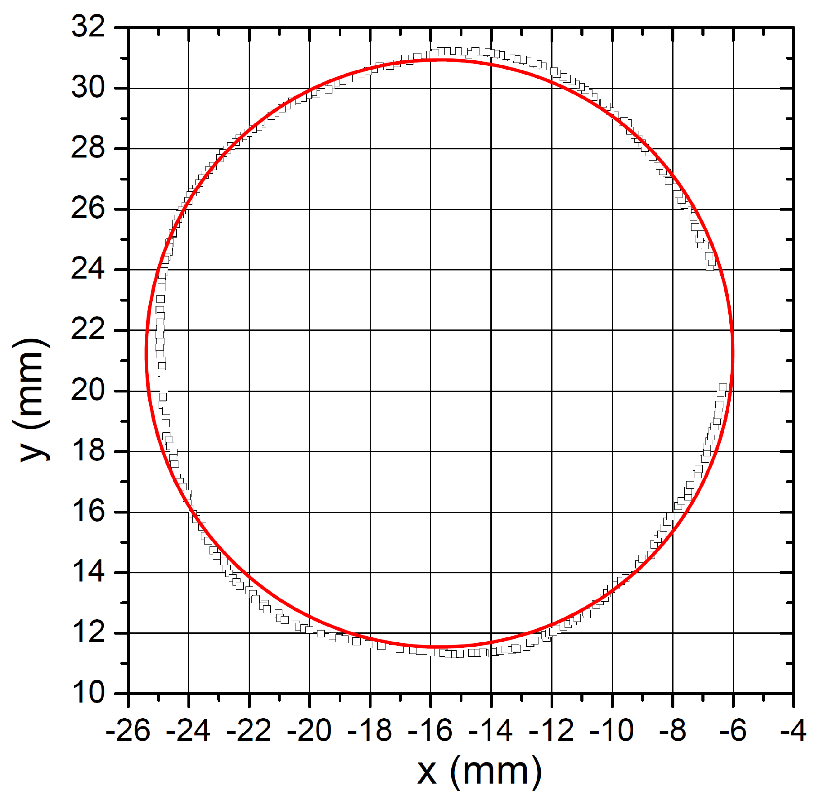
Figure 5 shows a reconstructed trajectory as it is obtained with the sensor array in static condition and the dipole (which is radially oriented) that rotates on the
mm plane. Imperfect parallelism between the sensor plane and the trajectory plane can make the trajectory projection slightly elliptic. However, a simplified model is sufficient to appreciate the performance of the system. With a simple circular model, we obtain a best fitting trajectory (see the red line in
Figure 5), corresponding to a RMS error as low as 0.4 mm over a 21 mm diameter.
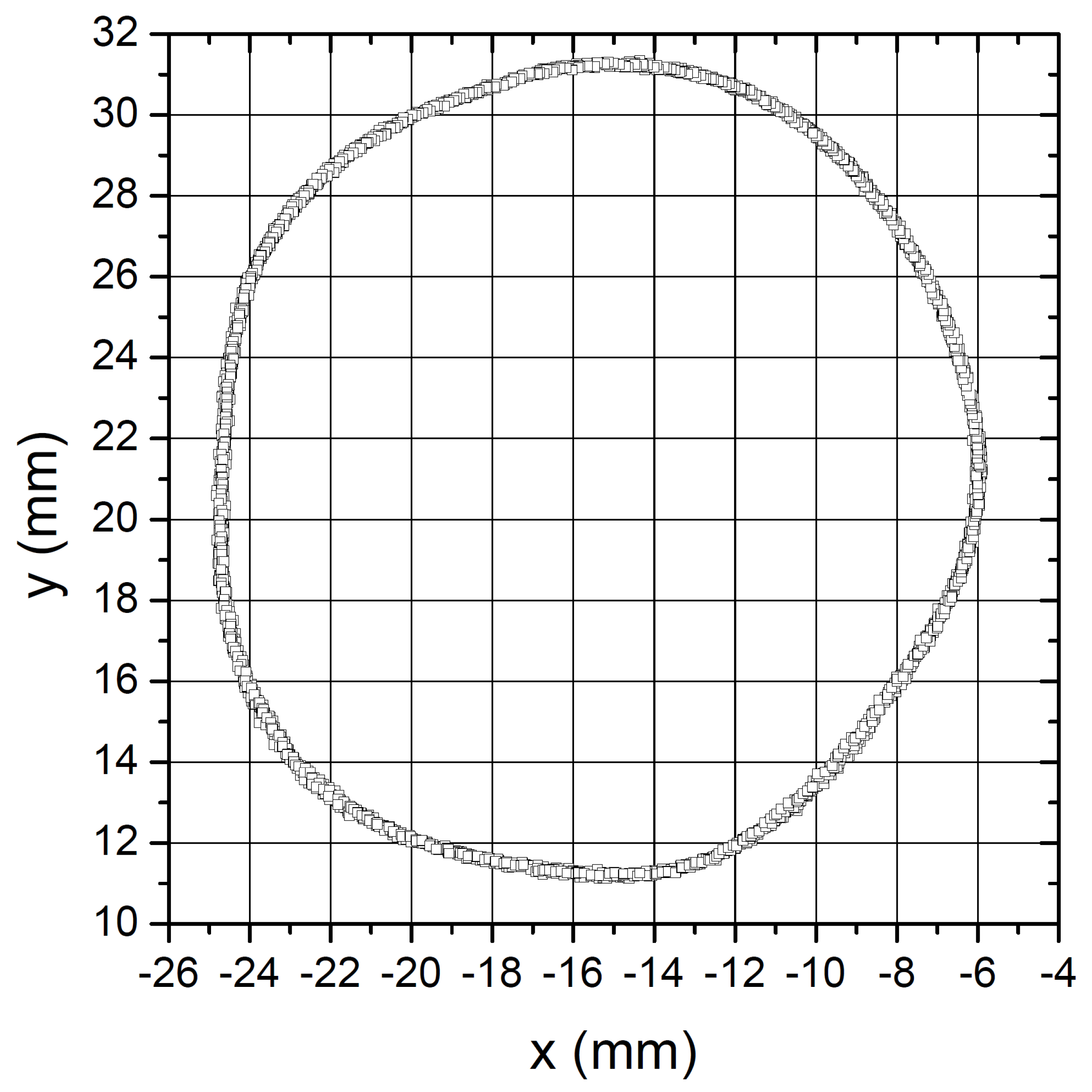
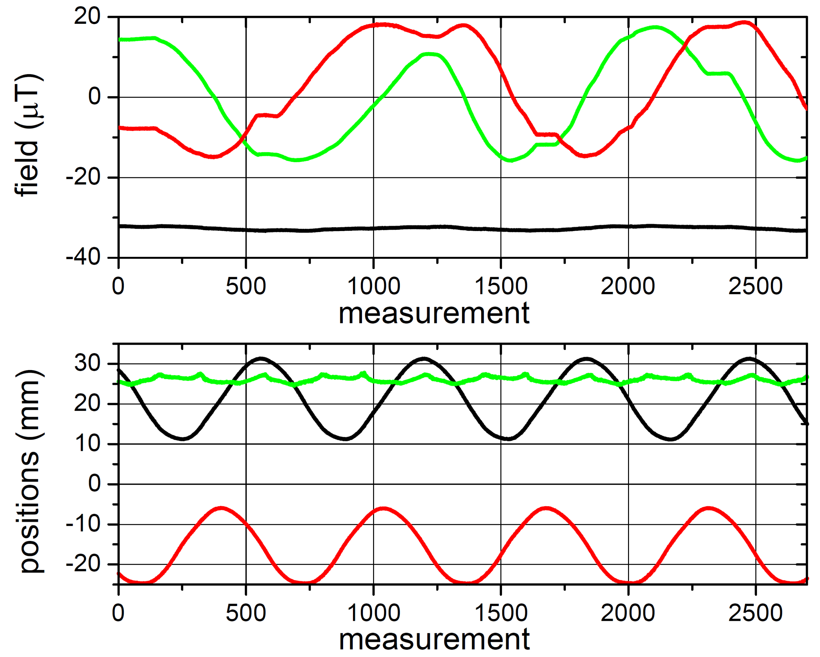
Figure 6, upper plot, shows a reconstructed trajectory obtained with the magnet performing a similar circular trajectory on the
mm plane. This time, the sensor array, which is rigidly assembled with the magnet driver, is held in the hand and moved freely, to test the robustness of the measurement with respect to the reorientation in the environmental magnetic field.
The motion applied to the assembly is approximately a rotation (about one turn backward and forward) around the
x axis. In this case, the system measures the environmental field with significantly changing components, whose values are represented in the middle plot of
Figure 6, as evaluated throughout the tracking procedure. Finally, the bottom plot shows the corresponding time evolution of the position co-ordinates. The figure proves that the reconstructed trajectory is negligibly disturbed by the array being in motion. The experiment is performed in a “normal” room containing furniture with ferromagnetic frames, computers, and other sources of potential magnetic interference.
Preliminary quantitative estimates of the position uncertainty are based on the variance of the 3D position detected—under static conditions, we measure a root-mean-square (RMS) of 131 μm when the magnet is held still on the z axis, at mm. Under these conditions, the relative RMS of the environmental field measured and of the dipole modulus are and , respectively.
The same kind of estimation, performed when the assembly is hand-held and freely rotated, gives μm and . In short, the position tracking is robust and sub-millimetric both when the array is kept static and when it is randomly reoriented with respect to the environmental field. The small variance of the dipole modulus estimations indicates that the system has a good degree of robustness with respect to ambient field variations. In addition, the environmental field inhomogeneities typical of normal working rooms do not constitute a problem. In contrast, the tracking system fails when magnetized devices get too close to the sensor array.
We notice an unexpectedly large variance in the dipole modulus estimation when the magnet moves with respect to the sensor array. For instance, in the case of the trackings in
Figure 5 and
Figure 6, we achieved
values of about 7.6% and 9.8%, respectively. These large values could be ascribed to small uncertainties in the positions of the sensors as well as to non-linearities in their responses. Despite this large variance in the dipole estimation, the quality of spatial tracking in
Figure 6 is comparable to that in
Figure 5: notably the greater uncertainty in the dipole vector determination is not associated with a significant degradation of the position tracking.
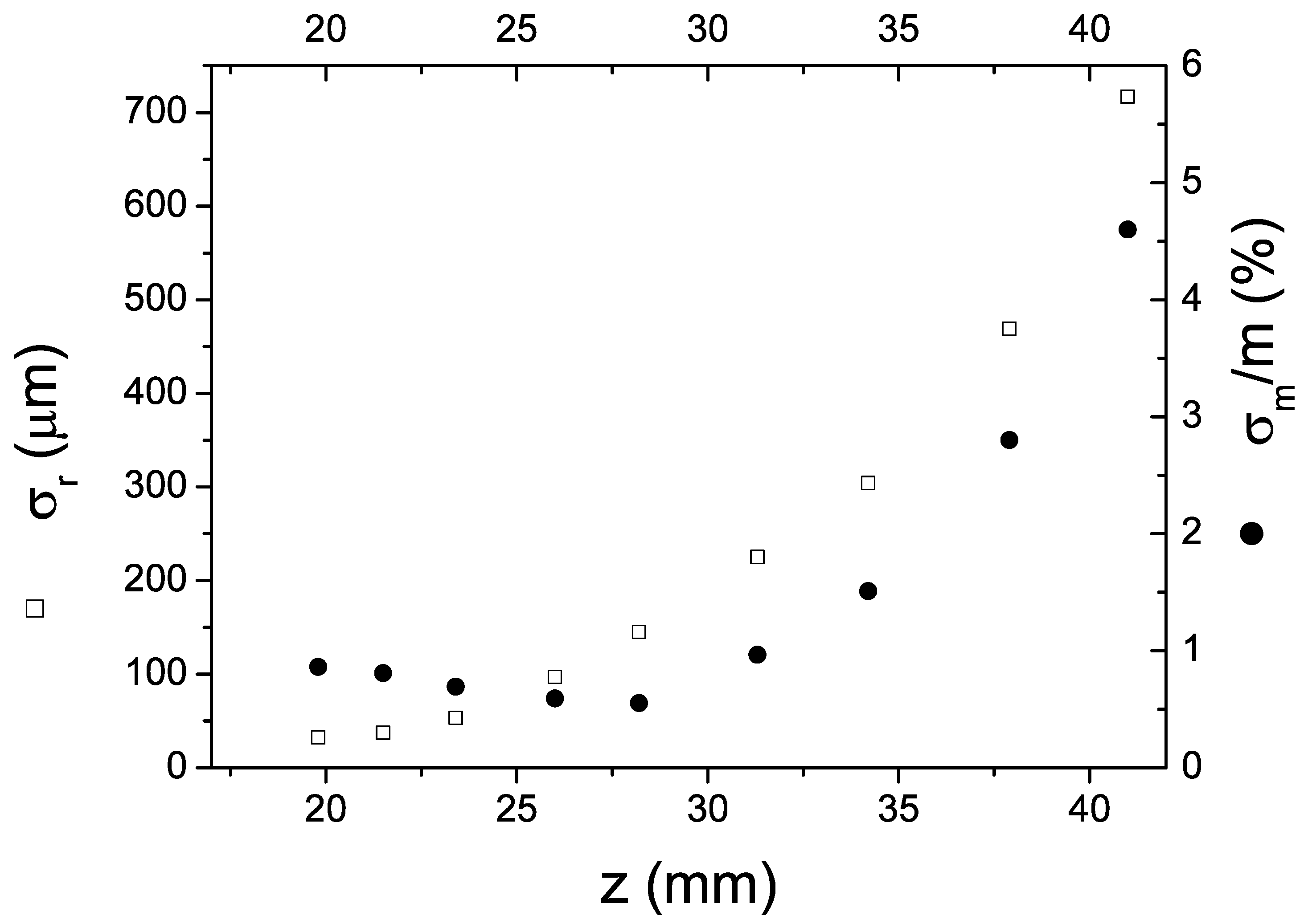
As expected, the tracking performance with a given magnet drops dramatically when it is displaced too far from the sensor array, making the dipole field comparable with the system noise, or too uniform over the array size. This behavior is effectively confirmed by the data plotted in
Figure 7. This figure shows the absolute position error (RMS of the reconstructed position) and the relative RMS of the dipole modulus as a function of the
z co-ordinate of the magnet, that is, at increasing distances from the array.
Concerning the speed, we proved that the system can acquire and track continuously at the maximum sampling rate (currently set by the firmware at 100 Sa/s) on a standard personal computer (e.g., on an i5-7400 CPU, 3 GHz, 64 bit).
12. Conclusions
We have built and tested cheap and reliable hardware based on commercial magnetoresistive sensors that, after appropriate calibration procedures, provides a set of 24 magnetometric measurement data at a rate as high as 100 Sa/s. The hardware contains a microprocessor enabling immediate data transfer to a personal computer, which in turns executes data elaboration to extract multidimensional (from 7D to 9D) spatial and angular co-ordinates of the magnetic source with respect to the sensor array and of the latter with respect to the ambient field. The tracker is scalable in size and may be of interest for various kinds of applications, ranging from medical diagnostics to virtual and augmented reality.
13. Patents
The subject of this work, in virtue of its interesting potentialities and of its demonstrated performance in terms of precision and speed achieved, constitutes part of the contents of a recent patent application [
30].

 ,
, 


