Analyzing the Effects of Tactical Dependence for Business Process Reengineering and Optimization


School of Engineering and the Built Environment, Anglia Ruskin University, Bishop Hall Lane, Chelmsford CM1 1SQ, UK
*
Author to whom correspondence should be addressed.
Designs 2020, 4(3), 23; https://0-doi-org.brum.beds.ac.uk/10.3390/designs4030023
Submission received: 30 May 2020
/
Revised: 1 July 2020
/
Accepted: 6 July 2020
/
Published: 7 July 2020
Abstract
:Implementing business and manufacturing process reengineering is challenging and poses major issues. The dependence issues between process functions during the implementation phase are the main reason for the high failure rate of process reengineering. The incompetence in identifying the dependence makes existing business process reengineering approaches static for modern business and manufacturing process structures. This paper has implemented a new process reengineering approach called the Khan–Hassan–Butt (KHB) methodology that incorporates the process interdependence algorithm to identify the dependence issues. The KHB method is a hybrid process reengineering approach to identify dependence issues before implementing changes; thus significantly reducing the failure rate of implementing business process reengineering. The KHB method has been implemented in a Bangladesh fabric manufacturing facility. The mapping and verification of the process have been completed using the WITNESS Horizon 22.5 simulation package. The case study has investigated the fabric production process and identified the dependence issues between each function and suggested changes to optimize the process. The outcome has shown significant improvement in production output and process efficiency.

1. Introduction
Business process reengineering (BPR) is a strategic tool for managing, analyzing, and designing workflows as well as business processes within an organization [1]. BPR has established itself as a comprehensive management tool for the development of business processes [2]. In recent years, much work has been done to study factors that influence the implementation and performance of the BPR [3]. The Hammer and Champy’s BPR methodology (Business system diamond), Davenport’s and Short’s Methodology, process analysis and design methods (PADM) framework, and Jacobson’s methodology (objective-oriented methodology of BPR) explain the core process and objective of BPR [4,5,6,7,8,9,10,11,12,13,14,15,16,17,18,19,20]. Hammer and Champy describe the reengineering objective as “achieving dramatic improvements by redesigning the fundamental business process” [21]. PR identifies the process as the main subject to be reengineered to reduce costs and inventory assumptions [22]. On the other hand, Davenport and Short described BPR as a consistent performance of the task to accomplish the business goal [23]. They derived reengineering processes in terms of organizational goals through optimizing processes and subprocesses to increase productivity. The PADM framework defines the analytical process and design methods of BPR [4]. PADM framework identifies the goal of the reengineering process and technical boundaries as the most critical task to be accomplished. It provides a framework to reduce complexity, nonvalue adding steps, and improve control of variances between business functions [4,5,6]. Jacobson’s objective-oriented method identifies the object orientation of a company in terms of products, processes, and services [4,22]. Jacobson defines BPR in two steps, reverse or backward engineering, to develop the existing process and forward engineering to design a process of new product or service [4,22,23]. Apart from these four methods, other proposed methodologies do not address the change in the core process of BPR. Most of them consider factors that influence BPR in terms of the management perspective that can instigate risks [7,8,9,10,11,12,13,14,15,16,17,18,19,20]. In terms of organizational culture, process reengineering represents tools and technique for management by bringing significant changes in the operations procedures [1].
With the development of PR protocols, the need to identify their failure factors also became important. These failure factors represent the rigidity of processes against changes for successful implementation of management strategies to achieve improvements. The failure factors are considered to be the main reason for the high failure rate of BPR methods. The failure factors vary based on the types of organizations and tasks needed to implement changes. The inability to identify the failure factors is a major strategic limitation of the existing BPR methods. Most of the current BPR methods do not have a contingency plan to solve the problems that occur because of the dependencies between tasks leading to the establishment of a different set of failure factors [7,8,9,10,11,12,13,14,15,16,17,18,19,20,24]. Although the failure factors are dependent on the task, there are some common factors such as cultural, structural, strategic, and people, which can be investigated regardless of the task [25,26,27,28,29,30]. The rigidity to change management and cooperation are the main cultural failure factors of BPR as these create obstacles on the way of BPR implementation. PR requires the coordination of people, processes, and technology to set a clear vision and values [29]. In most organizations, the main reason for failure to harmonize the integration of crucial success factors is management rigidity for bringing changes. Furthermore, the lack of communication initiates cross-functional dependence and rationale that are reciprocal to each other [4]. Magutu, Nyamwange, and Kaptoge [30] derived unsuccessful cooperation of manufacturing and human resources, notably large working groups and the practice of collaboration, as success or failure factors of BPR.
The tactical dependencies of BPR arise during the implementation phase and could either increase the efficiency or create obstacles [4,5]. Different methodologies of BPR reveal that some degrees of dependency exist in every step and substep of a reengineering process [1,30,31,32,33,34,35,36,37,38]. The dependence issues can drive the BPR effort towards success or failure [39]. In the manufacturing process, the dependence issues can be termed as process interdependence (PI). They are cross-functional and have a significant impact on organizational performance and productivity [4,5,30]. Based on the structure of the organization and manufacturing process, the tactical dependencies issues can be formed in three different types, i.e., pooled interdependencies, sequential interdependencies, and reciprocal interdependencies [5,11]. The first type exists in the process functions and is initiated separately.
Furthermore, they may not be dependent on each other in terms of execution. These types of processes have blind dependence on the performance of every unit. The second type of interdependencies defines dependencies issues, while the performance of one section impacts the performance of the overall process. Manufacturing and production processes are sectors where sequential interdependencies exist. In the third type, dependence issues arise when the output of a department becomes the input of the subsequent department. In a business organization and process, reciprocal interdependence defines dependence aspects. Reciprocal and sequential interdependencies sound almost similar; there are differences in terms of performance and impact on the overall process [5].
Although the existing BPR methodologies are capable of developing a solution, they are limited as they only consider required changes for an organization and do not include evaluation of the current process [4,40]. For example, the PADM framework does not incorporate process evaluation but uses the strategic business context to design the reengineered model. In the existing BPR models, the improvement of the procedure is the main focus, and the key performance indicators are improved incrementally [30,31,32,33,34,35,36,37,38]. However, the identification and integration of dependence issues can result in a better outcome. The main four methods of BPR do not have an identification process of the dependence issues between department and section; thus making the implementation of BPR more vulnerable to the interdependent problems that arise because of the reciprocal and sequential interdependencies in a process. Most of the BPR methodologies do not consider continuous process improvement (CPI) [5]. Apart from the PADM framework, all other methods become static during the implementation phase because of a lack of a contingency plan for CPI. One of the most significant limitations of the existing BPR methods is that they are not well-structured and do not follow a step-by-step procedure [30,31,32,33,34,35,36,37,38]. Most of the current BPR methods explain BPR in terms of the organization, not in terms of types of organization and processes [30,31,32,33,34,35,36,37,38]. The sparse structure is one of the most vulnerable characteristics of the existing BPR methods. Different research and BPR methods show the reengineering process of an organization, both service and production [7,8,9,10,11,12,13,14,15,16,17,18,19,20,41,42,43]. However, they do not have a competitive structure to reengineer the manufacturing/production process. Taken together, these factors make the existing BPR methods vulnerable to failure. Most of the BPR methods use IT as a primary tool for improvement without any proper strategy of using the right technology in the right place [40,44,45]. Without proper evaluation and a contingency plan of continuous improvement, it will be hard to achieve consistent results [23]. Automation and software development tools do not take into consideration the dependence issues to visualize the business and process model [44]; this adds another layer of challenges that stems from the inability to accurately identify interdependent factors, dependencies, issues. Dependence issues can exist between the processes from the beginning of the BPR initiation. They may also arise when a change is made in one section of a process. None of the existing BPR methods is well-structured to identify dependence issues, and these are considered to be the reason for a 70–80% failure rate of the existing BPR methodologies [40,44].
Research has revealed that 67% of the business leaders use existing BPR methods as tools for BPR projects in an organization [40,44] even though they experience a failure rate of 70–80%. The existing BPR methods are not competent enough to decrease this failure rate as they do not have a core process and strategic plan to identify and face the critical dependencies issues during the development plan [4,5]. Thus, problems occur due to intricate structures, dependencies between the departments, and lack of resources. All the discussed BPR methods have two significant limitations. First, none of them has a step-by-step procedure and implementation process for an entire organization. Second, the methods do not have a contingency plan or process that can consider and identify the dependence issues of BPR [45]. These issues can be solved by establishing a process that is structured and can take into consideration the interdependency issues of different sections within the manufacturing process. In our previous research, we proposed and discussed a combinational approach of structured data-driven process reengineering method and an interdependence algorithm known as the Khan–Hassan–Butt (KHB) method. The method utilizes simulation tools and can be applied to business processes as well as manufacturing processes [4,5].
One of the major problems with real-life optimization is the prevalence of uncertain data. There could be many reasons for data uncertainty including measurement errors, lack of knowledge, and implementation errors in a real process set-up [46]. There are approaches to deal with data uncertainty e.g., stochastic and robust optimization. In stochastic optimization (SO), the most important assumption is that the probability distribution is required to be known and estimated. On the contrary, robust optimization (RO) does not ascertain the probability distribution as known functions [47,48]. The computational tractability made the RO a very popular method for uncertain data sets and problem types. RO is used in different fields such as management, engineering, healthcare, and finance [46]. In addition to RO and SO, simulation-based optimization techniques are also quite popular for process optimization [49]. Among the simulation-based optimization methods, the statistical ranking and selection (R/S) method is commonly used for known problems and alternatives. In this method, simulation is used to measure the system’s performance [49]. A heuristic method is used to speed up accuracy and to solve problems. The main goal of heuristic methods is to find solutions faster than traditional methods. In a heuristic method, a local optimal is used and it is considered as a close approximation for the final solution instead of the optimal value [50]. Apart from these methods, there are stochastic approximation and derivative-free optimization methods as well. These methods are applied in the optimization process where the derivatives are not available or uncertain [51]. One of the main limitations of these simulation-based models is their inability to instill a dynamic behavior for a model to represent the existing process [52]. Another problem is the complexity that arises due to uncontrollable parameters between the real-world and the simulation models. The statistically estimated parameters make it more complex to determine the objective function [53]. The KHB method uses simulation as an IT tool for mapping and analyzing the process. It includes a verification step to verify the simulation model with real-world data. It uses a process interdependent algorithm (PIA) that identifies areas of interdependency (Section 2). The data set collated from a manufacturing process is extremely large and requires processing to extract actionable information. To remedy this issue, the KHB method utilizes a data filtration process (DFP) to filter the large data set into a small number of convenient parameters. One of the main features of the KHB method is that it identifies the interdependence factors from the process itself and filters them into actionable information using the DFP (Section 2). Much work has been done for optimizing process (manufacturing) using a simulation-based optimization technique in different sectors such as operations, management, engineering, and manufacturing [54]. For example, Dengiz and Akbay optimized the production line of PCB manufacturing facilities by 12% through an investigation into the effect of batch size push-pull [55]. They used simulation and regression metamodeling analysis to optimize the batch size problem. On the other hand, Syberfeldt and Lidberg used the cuckoo search to optimize real simulation-based manufacturing [56,57]. They identified different optimization problems and used a metaheuristic algorithm to optimize machine utilization by 15% [56]. These examples show the applicability of simulation-based optimization techniques for manufacturing.
The interdependencies between functions can be modeled based on their types. In our previous research, we identified and optimized the reciprocal interdependence between the functions of a production process using a data-driven process and PIA [5]. We used the KHB method to optimize the production process of ACME valve manufacturing. The production process was previously optimized and validated by other researchers. They made use of an expert mechanism that can identify bottlenecks and recommended resources accordingly for optimized processing [58]. A comparison between the expert mechanism and the implemented KHB method showed an increase of 20% in output using the same amount of resources [5]. This shows the superiority of the KHB method over traditional bottleneck and optimization approaches. In this research, we have used the KHB method in a sequentially interdependent production line to identify the impact of dependence issues. The PIA used in the KHB method identifies the dependence data of the process based on specific boundary conditions that can have a positive or negative impact on the process. The data filtration process (DFP) filters the dependence data into actionable information based on the positive and negative impact on the process; thus, the changes to optimize the process becomes more accurate and efficient. The main contribution of the work is the effective implementation of the KHB method to identify sequential interdependency within the process for its optimization and failure rate reduction in an established Bangladesh garment manufacturing facility as a case study.
2. Methodology
This research aims to implement the KHB method in a Bangladesh garment manufacturing facility. The methodology will explain how the interdependencies are overlooked in a conventional optimization approach and make the process optimization vulnerable to failures in the long run. It will provide a step-by-step procedure for identifying dependence issues, and how the new hybrid process reengineering approach (KHB method) can integrate the dependence issues to reduce failure percentage.
KHB Methodology
The KHB methodology is the integration of data-driven process reengineering (DDPR) and process interdependence algorithm (PIA) [4,5]. The KHB method incorporates process reengineering data analytics as an approach of hybrid process reengineering for both business and manufacturing processes. The KHB method can integrate dependence issues of process reengineering and is capable of providing better output as well as decreasing the failure percentage. The structure of the KHB is shown in Figure 1 [5].
The KHB methodology shown in Figure 1 comprises five main steps. The first step of process identification represents the operation management of the process. It is intended for two purposes. Firstly, to provide a generic model for process mapping and verification. Secondly, to provide hypotheses and equations for process verification and reengineering. Process mapping starts with gathering quantifiable and quality data that is the backbone of the process to represent a formal structure of the existing process flow. The process is mapped from the collected data of the business process or manufacturing shop floor. This section identifies a process based on the layers and steps, workstation or department capacity, lead time or delivery time, idle time, or the set-up time of the process.
In the verification process, the collected data is compared with previous data for accuracy. However, in this research, we have used simulation packages as IT tools and experimentation platforms before implementation and showed the verification process by comparing the simulation data and actual process data. Process verification is the identification process to find out if there is an error in the process mapping as wrong data and structures will provide wrong information of the process, which may propagate failure to the reengineering initiatives.
Once the process verification is done, the reengineering phase starts with the identification of dependence issues between workstations or departments that can be termed as process interdependencies of the process. The methods are designed for identifying reciprocal and sequential interdependence which are common in business and manufacturing processes. The KHB method uses structured data analysis through the process interdependence algorithm (PIA) to determine the dependence issues. The reengineering section identifies the dependence issues and uses them as decision-making tools for optimizing the performance. In the process of identifying the PI, the structured data are filtered based on some boundary conditions. The boundary condition used in this work is as follows.
- Interdependent if changes affect any of the similar factors between two sections (idle%, busy%, block%, number of operations/transaction), and increase the number of operations.
- Interdependent if changes affect any of the similar factors between the sections (idle%, busy%, block%, number of operations/transaction), and decrease the number of operations.
- Not interdependent if changes affect any of the similar factors between the sections (idle%, busy%, block%, number of operations/transaction), and the number of operations is unchanged.
- Not interdependent if the changes do not affect any of the similar factors (idle%, busy%, block%, number of operations/transaction), and the number of operations is unchanged.
The defined boundary conditions help in filtering the data using PIA. The data used in this research are structured data. The PI identifies the data set and information that has a significant impact on the process. However, this impact can be either positive or negative. The boundary condition is the decision-making criterion that separates the negative and the positive impact; thus filters the data that contains the information of changes required to optimize the operation of the process. This filtered data set can be implemented directly for increasing process efficiency and is termed as smart-structured data (SSD). The filtration process from the PI data set is described in Figure 2.
Figure 2 represents the data filtration process, along with the identification of interdependent and not interdependent factors. The PIA uses the structured data from and the four boundary conditions: a, b, c, and d. The boundary condition separates the interdependent (conditions “a” and “b”) and not interdependent (conditions “c” and “d”) factors. The interdependent factors are again filtered based on conditions “a” and “b” to measure the positive and negative impact. The positive data sets are the factors that can be implemented directly to increase the process efficiency.
Once the interdependence data is filtered to SSD, the next step is the pilot run of the process to validate the accuracy and efficient use of resources. The pilot run process is the bridge between the reengineered model and implementation. In this section, the output of the small scale implementation or simulation Ns is compared with the existing model output Nr. And the validated output and factors are suggested for final implementation. Once the changes are implemented, the evaluation process compares the output of the reengineered and existing model. The process analysis is the analysis of the reengineered model for further development to decide by the management. In this section, management decides whether they stop the reengineered process and standardized the implementation or go for a further cycle for continuous improvement process (CIP) based on available factors such as resources.
All these steps of the KHB method have been used to conduct a case study in a garment manufacturing facility in Bangladesh with the aim to identify interdependencies and reduce the failure rate of the BPR method that can optimize the process flow and increase productivity.
3. Case Study
The KHB method is implemented and validated using a garment manufacturing facility in Bangladesh as a case study. The fabric manufacturing company is a 100% export-oriented facility and exports all categories of ready-made garments (RMG) for men, women, and children sportswear over 29 countries. It has two separate sections for fabrics and ready-made garments. The current production capacity of ready-made garments (RMG) is 130,000 pcs/d. It has national and international recognition from OEKO-Tex, organic cotton standard (OCS), ISO 9001-2008, SEDEX, and BSCI.
The data was collected directly from the shop floor, and the process was mapped based on process identification and structured data. The production line data were structured and used for process identification and mapping without any modifications. The process flow of the studied tubular fabric production process is described in Section 3.1. The implementation of the KHB method for the production line reengineering and optimization is described in detail in the subsequent sections based on the KHB methodology.
3.1. Process Identification
This case study identified the finishing process of fabric manufacturing for the experiment and case study model. The whole process is sequentially interdependent as one section must accomplish something before the next section can do its task. The finishing section has different units from squeezing wet fabrics to shipment of finished goods. There are two types of fabrics produced in the finishing section, i.e., tubular fabrics and open fabrics. The tubular fabrics are tubular in shape and produced based on the required diameter for different garments wear. The tubular fabrics are cut open to open fabrics for customization of garments wear that requires stitches. The tubular fabrics are cut open in the squeezing section for the open production line.
The finishing section has two separate production lines for tubular and open fabrics. The tubular and open fabric production lines are entirely independent and are not cross-functional. For validation and implementation, the tubular section has been analyzed in this case study. The finishing process is identified based on the operations and has five different parts as follows.
- Dewatering section (P);
- Quality inspection wet (Q);
- Drying section (R);
- Quality inspection drying (S);
- Compacting section (T).
The process identification based on the data and working procedure is shown in Figure 3.
The dewatering section initiates the first function of the finishing section by receiving wet fabrics and trolleys from a stock buffer. It has two machines with a similar cycle time of 60 min/250 kg fabrics. The quality inspection takes a sample from the squeezed fabrics and examines them for any unwanted marks or discoloration and diameter. The cycle time is relatively low as it takes only one sample from similar types of fabrics coming from the same machine. The cycle time for both sections was decreased and increased by up to 20% to track the changes in idle%, busy%, number of operations. The drying section pulls fabrics from the tub stock buffer. There are three machines for drying sections where hot air at 70–80 °C is blown to dry the fabrics. It has a straightening and unloading section integrated with the machine. The dry fabrics are quality inspected for color and diameter by taking the sample from trolleys. After quality inspection, the fabrics are pushed to the tub dry buffer from where they are pulled by the compacting machines. There are three compacting machines which compact the fabrics and send them for packaging. The packaging is not part of the finishing section as compacted fabrics go for final quality check and weight and then packed in the offline quality inspection area.
3.2. Process Mapping, Data Collection, and Analysis
The finishing section produces an average of 9200 kg/1380 min. The production line runs for 24 h with one hour of break time. The tubular trolley can hold a maximum of 300 kg of wet fabrics. In the tubular section, the process starts with receiving fabrics from the stock buffer. The dewatering machines squeeze the wet fabrics. There are two dewatering machines with similar cycle time. They maintain a speed of 4–5 m/min depending on the diameter and thickness of the fabrics. The squeezed fabrics go to the stock area for quality inspection. After the quality inspection, the drying section dries the fabrics with three drying machines. The drying machine blows air at a temperature of 70–80 °C. The process has a rolling speed of 10 M/60 s. The dry fabrics go for second quality inspection for color, diameter, and % of shrinkage. The process has a 2–3% of wastage. The drying process is an integrated process where it is required to straighten the fabrics that take an average of 2 min and another 2 min to offload from the machines. The straightening and unloading processes are fixed and integrated with the drying process. The compacting machine has a straightening and unloading section combined with the system similar to the drying machine. It compacts the dried fabrics. During the compacting, the tubular fabrics are checked for quality online and sent directly to packaging for shipment.
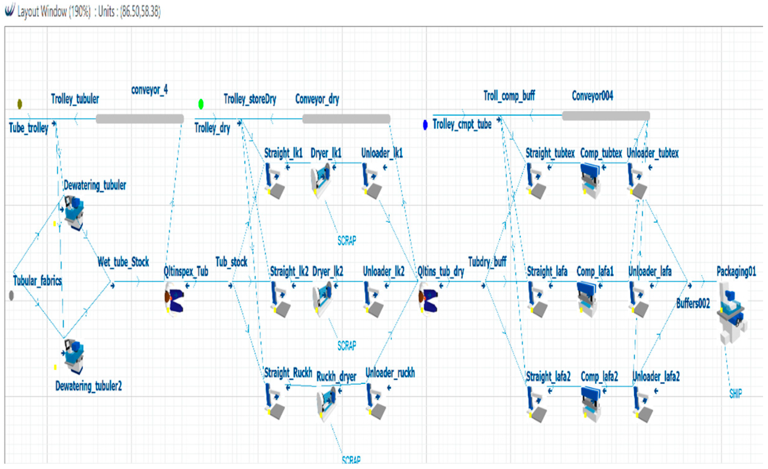
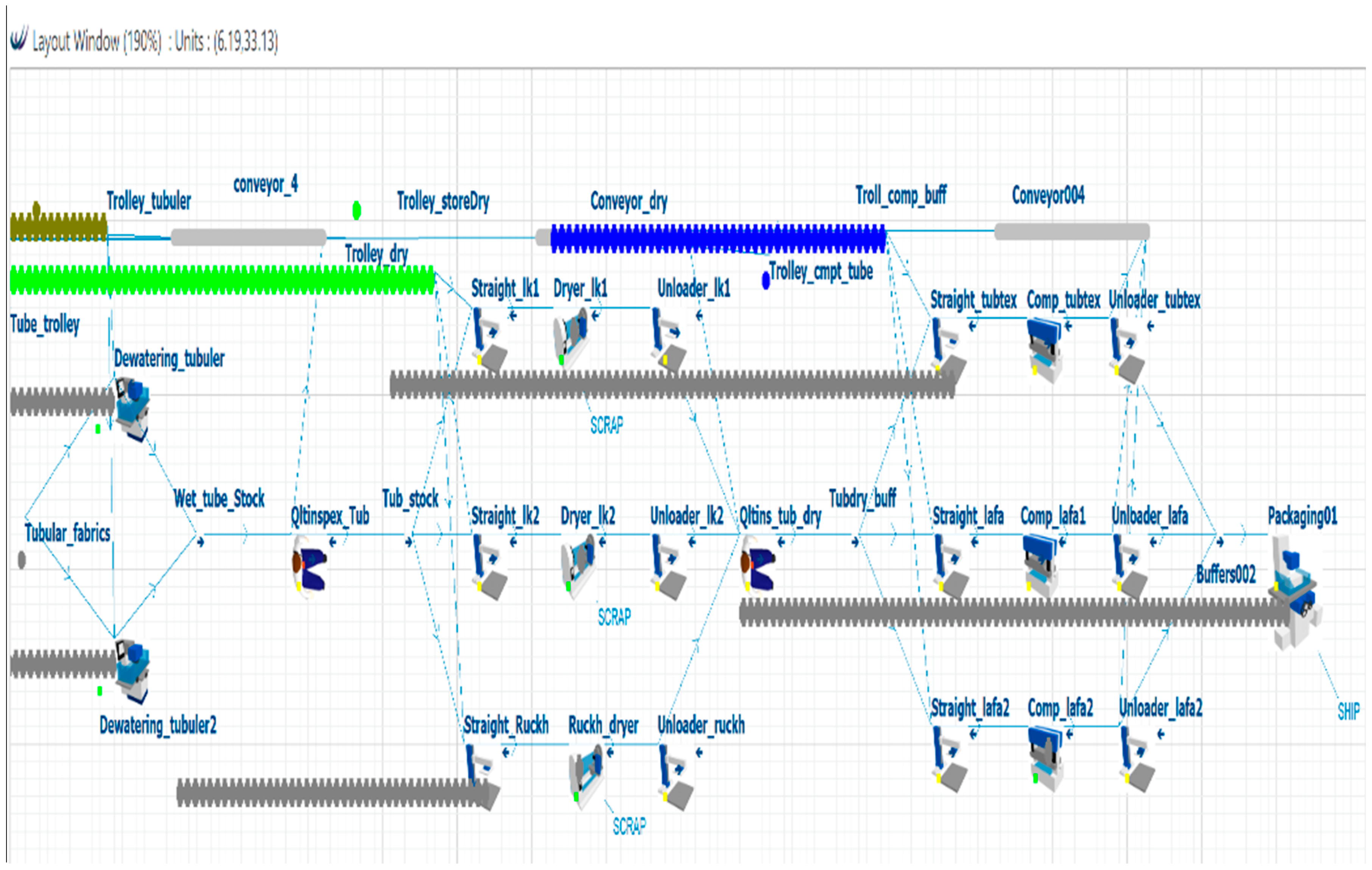
The process mapping and the data were collected from the shop floor for three weeks of production. The analysis and comparison of the past six months’ data with the collected data ensured the accuracy and efficiency of the data. The WITNESS Horizon 22.5 simulation package was used to map the process. Figure 4 represents the process mapping of the tubular fabric finishing process. The capacity of the production line is measured using a continuous flow of raw materials.
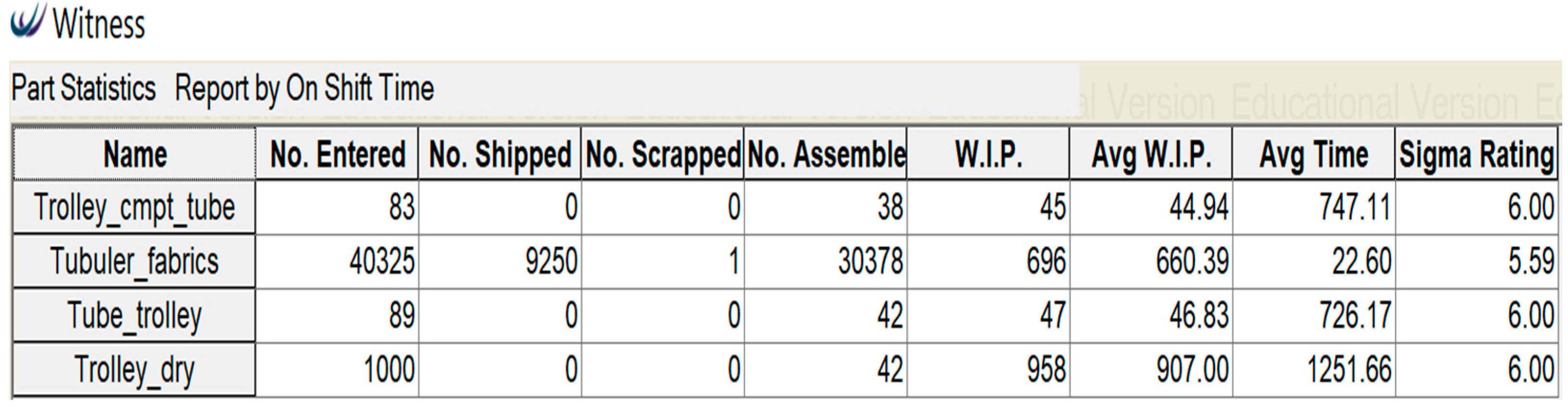
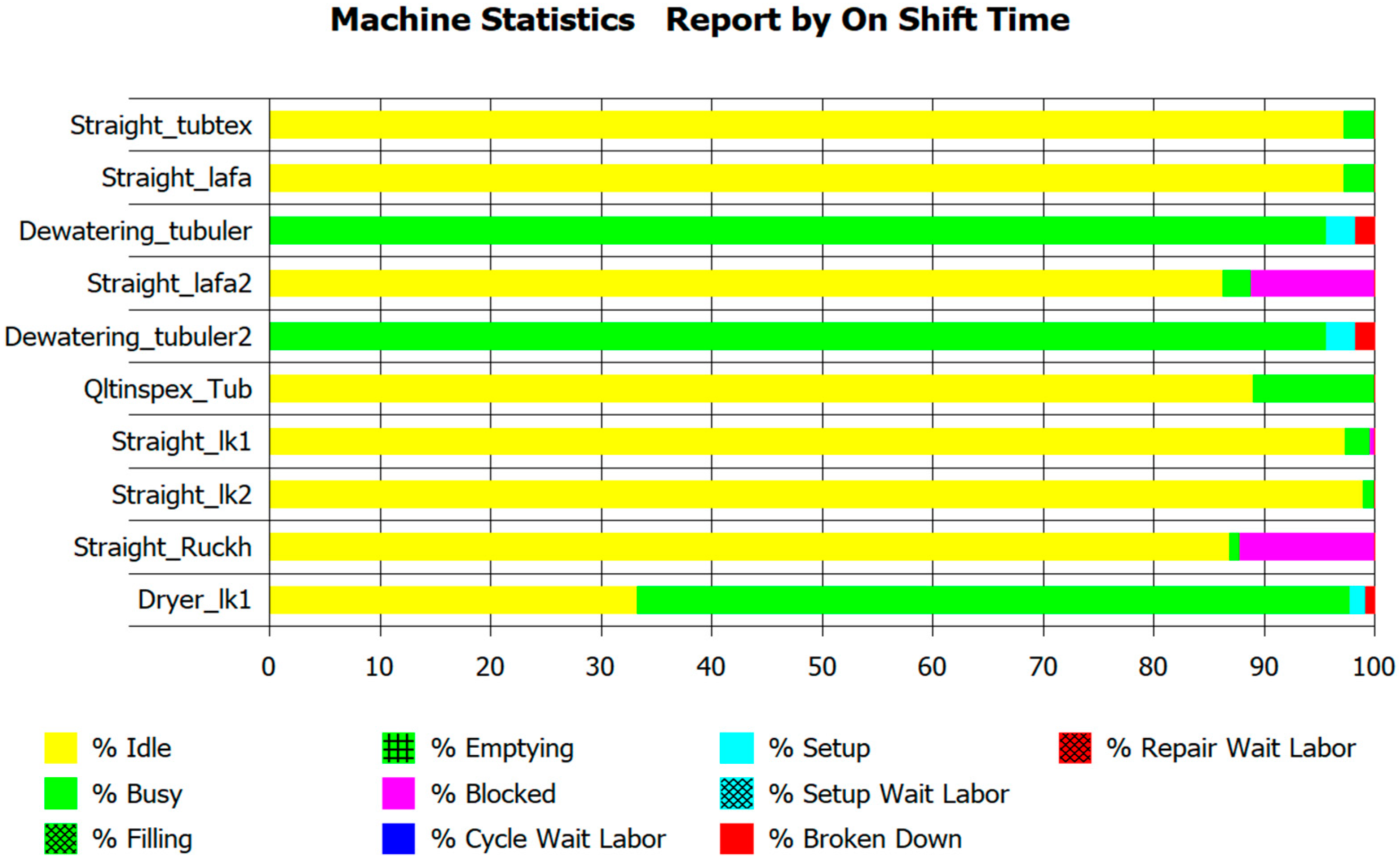
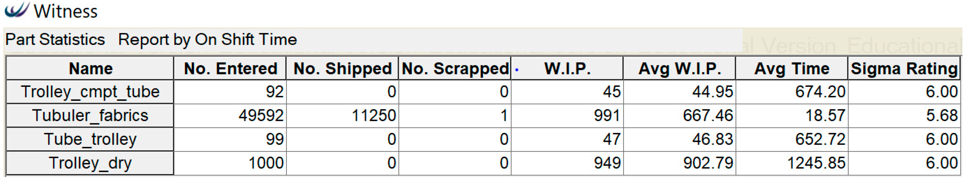
The maintenance, set-up, and break down time were calculated from the shop floor data and compared with the previous data to ensure accuracy. Some of the maintenance takes place once every two weeks. To get accurate data for the breakdown, set-up, and maintenance, the calculated data were compared with the past six months’ data, and an average was taken for the simulation. The tubular production line produces an average of 9200 kg/d, according to the recent six-month data. The witness model output of the tubular production line is shown in Figure 5. Figure 5 shows the daily production as no shipped and working in progress (W.I.P) information for the trolley and tubular fabrics. It also shows the average W.I.P and time for a day (1380 min) of operation. The simulation model has a production of 9250 kg/1380 min or a day of operation. The difference between the average and the calculated data was within 5% of set-up and breakdown time. Figure 6 shows the machine statistics for different time parameters of the production line.
3.3. Process Verification
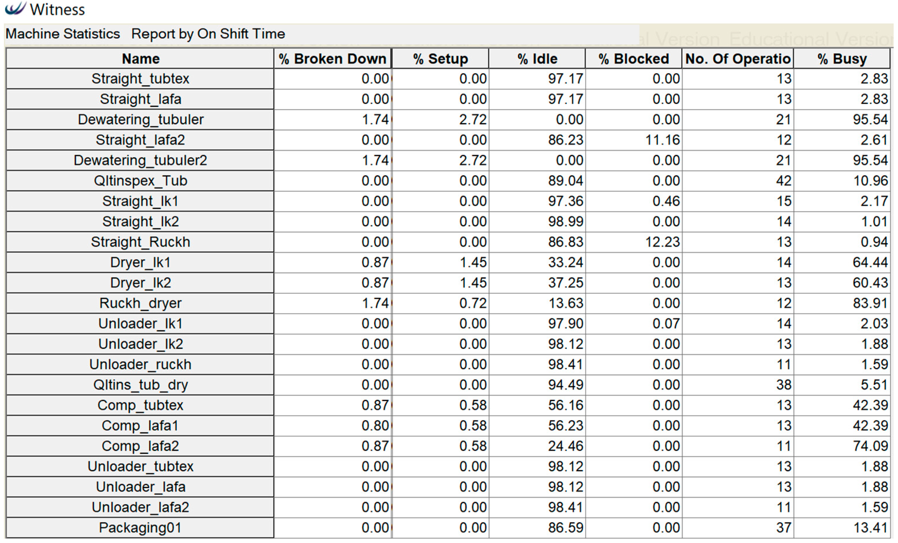
The simulation model is designed based on the machine set-up and operations data collected from the shop floor. The process can be verified by analyzing the flow of parts and output. The average data was used for setting up breakdown and maintenance time. The simulation model provided the production of 9250 kg/d, which is close to the average of 9200 kg. The production line starts with the dewatering and finishes with the compacting section. For verification of the process, the output of the compacting section is calculated for the actual production line and simulation model. Figure 7 represents the idle percentage, blocked percentage, busy percentage, no of operations for all the machines, and set-up for the finishing process.
In Figure 7,
- Comp_lafa1 busy time, Ccb1 = 42.39%
- Comp_lafa2 busy time, Ccb2 = 74.09%
- Comp_tubtex busy time, Ccb3 = 42.39%
- Rc = Process run time = 1380 min
- Comp_lafa1 Cycle time, Ccc1 = 45 min
- Comp_lafa2 Cycle time, Ccc2 = 90 min
- Comp_tubetex Cycle time, Ccc3 = 45 min
Then, the number of operations of comp_lafa1
- or,
- or,
Number of operations of comp_lafa2
- or,
- or,
Then, the number of operations of comp_tubtex
- or,
- or,
Total production from the compacting section from the simulation model = Ncp1 + Ncp2 + Ncp3 = 9250 kg
In the actual model, the total production average for the compacting section was as follows.
- Comp_lafa1 = 3200 kg;
- Comp_lafa2 = 2800 kg;
- Com_tubtex = 3100 kg.
The average production of the actual production line is 9200 kg. The difference is 0.54%. Thus, the simulation model can be verified as representing the exact model.
3.4. Reengineering Phase
In our previous research, we have shown the operational efficiency of the KHB method over traditional bottleneck optimization methods [5]. The main objective of this research is to identify the importance of PI for both optimization and operational efficiency. In this case study, the bottleneck is identified but not used for optimization; instead, dependence issues are identified using PIA. Furthermore, interdependencies are identified between all the workstations as the production process has sequential interdependencies. The bottleneck is determined to show the differences with the KHB method and explain dependence issues that are not covered by the traditional bottleneck approaches of optimization. The detailed analysis is done following the optimization method (KHB) described in Section 2.
3.4.1. Process Interdependencies
The process has been identified and mapped in Section 3.1, Section 3.2 and Section 3.3. For determining the interdependencies, the cycle time for each of the workstations is analyzed. The tubular fabric production has sequential interdependencies. The output of one workstation is used as the input for the consequent workstation as there is no subassembly in the process; thus, changes in one workstation have an impact on the entire process. The objective of finding interdependencies is to identify their impact and make changes accordingly. In the reengineering process, this interdependence is the dependence issue and causes failure to the BPR project as it cannot be identified with existing methods. The KHB method shows that these interdependencies that cause failure can be used to optimize the process better compared to the bottleneck approach if determined appropriately; thus, the KHB method identifies the dependence issues using PIA that streamlines the process and reduces the failure percentage. PIA filters out the data that affect the process in terms of cycle time, number of operations, busy%, idle%, block% of the machine, and use them for making changes to optimize the process. Cycle time of each workstation was decreased and increased by up to 20% to identify the impact and interdependencies of the subsequent workstation. The process interdependencies of the tubular production line are described in the next section.
3.4.2. Interdependence Factors between Workstations and Data Filtration
For identification of interdependencies between the workstations, cycle time has been used to track the impact of change on the entire process. In the simulation model, the cycle time is increased and decreased by 20%. The effect has been identified between all the workstations as interdependencies and stored as interdependent data sets. The optimization process followed the interdependencies as changing parameters. The boundary condition used for interdependence identification and optimization is provided in Section 2, and interdependence identification data are presented in Table 1, Table 2 and Table 3. Table 1 and Table 2 represent the interdependence relationship between P, Q, R, S, T. In Table 1 and Table 2 the interdependence relationship is presented by X ∩ Y, where (X, Y) = function of a process. The intersection indicates the common impact factors between two functions. X ∩ Y represents the set of interdependence between X and Y.
The tubular production line has five different workstations from the dewatering to compacting sections. The PI is identified for each of these workstations. Between the dewatering (P) and quality inspection (Q) section, the interdependence is recognized as the number of operations (Table 2). For decreasing the cycle time, the number of operations increases for both dewatering and quality inspection. The changes in the cycle time of the dewatering section have a significant impact on the entire process. Table 1 and Table 2 show the parameters interdependent and not interdependent between the dewatering and all other workstations. Table 1 determines that the current capacity of the drying section does not impact the dewatering section output. However, the dewatering section has a significant impact on the number of operations of the drying section, as shown in Table 1. The number of operations needs to be increased for increasing the overall performance.
A similar trend is found between the dewatering and drying sections. Table 2 shows that the dewatering (P), and quality inspection dry (S) are not interdependent. It implies that at current capacity, changes will not impact the output of “P” and “S”. Table 2 identifies that the number of operations is the interdependency between dewatering (P) and Compactor (T). At current capacity, changes in S will not impact the total output without making any changes in P as T P is an empty set as of Table 2. A similar analysis is done for all the sections for identifying interdependence. The interdependencies, along with the bottleneck movement, are drafted in Table 3 in Section 3.4.3.
3.4.3. Interdependence and Bottleneck Movement of the Process
The bottleneck of the process is identified to show the differences with the movement of interdependencies. The initial bottleneck of the process is the dewatering section which moves along with modification of the process. Table 3 shows the progress of the bottleneck of the entire process for a change in cycle time and resources; however, the interdependencies show the differences for a similar amount of change and support. From Table 3, it can be seen that the bottleneck of the process moves from the dewatering to compacting sections, compacting to dewatering and dewatering to compacting consequently. The traditional bottleneck approach does not consider the impact on the entire process for a change in a particular section. If we consider the interdependency from Table 3, P is interdependent with Q and S. Similarly Q is interrelated with S, R, and T. It shows that there are areas that are overlooked in the bottleneck approach. These overlooked issues are the dependence issues of the production process, which increase the failure percentage of the BPR project if not solved during the implementation phase.
Table 3 shows the interdependence between all the sections of the tubular fabrics finishing. It indicates that the bottleneck of the process cannot go through all the parameters that need to be considered to identify all the problems of the production process. The P is interdependent with Q, R, and S with the number of operations and idle% of machines; thus, any changes in P will affect Q, R, and S. While decreasing the cycle time of the drying section according to the interdependence will not affect the production. Preferably the process can produce similar output for a reduced capacity of the drying section until it matches the number of operations completed by the dewatering section. Similarly, for the other section, any modifications will affect the process, according to Table 3.
3.4.4. Optimization and Validation
The optimization for the tubular production line has been done considering the interdependencies. The reengineering process followed the dirty slate approach; thus, only implemented the changes possible within the available resources and considered the optimization of production within the current capacity without adding any additional machines. The process could not go beyond the capacity for validation of the process required to suggest the changes that can be implemented. The reengineering and adjustments made are based on the existing process capacity, so the production cannot go beyond 12,000 kg/d. The optimization model is shown in Figure 8. The modifications are made only in terms of cycle time, increased buffer capacity, and trolley management. No change in machine set-up was made. Figure 9 shows the output of the optimization model based on interdependence factors. The optimized output is 11,250 kg for 1380 min of operations. The data in Figure 9 indicates a 21.6% increase in the number of operations compared to the existing model output data in Table 4. The optimization model also has less production average (Avg) time (18.57) for tubular fabrics.
3.5. Implementation
The suggested changes based on Table 1, Table 2 and Table 3 are implemented through the modification of parameters in Table 4.
Table 4 represents all the modifications made based on the interdependence described in Table 3. The modified value provided an output of 11,250 kg. For the validity of the interdependence, the changes were suggested according to Table 3 and Table 4. The dewatering section’s cycle time was decreased by increasing the rolling speed by 5–10% based on the thickness of the fabrics. The changes are implemented mainly in the operations such as the arrangement of similar types and color of fabrics in machines which increased the busy% by decreasing cleaning time.
The trolley number was increased and fixed for loading and unloading to modify the blockage time. The modified set-up, cycle time, and set-up time provided an average production of 10,880 kg/d for seven days of operation, which is an 18% increase from the average output before implementing the reengineering process. The average production is 3.4% lower than the simulated output. The optimization can be done by identifying the PI between two side-by-side workstations or between all the workstations. The latter analyzes the process more precisely; thus, the accuracy will be higher, and the failure percentage will shrink. The process that has reciprocal interdependence should follow the former approach as reciprocal interdependence exists in two side-by-side processes. In the current case study, the fabric production process has a sequential interdependence, and the interdependencies are measured between all the workstations or functions. The interdependence functions have identified significant differences if changes were to be implemented based on the bottleneck approach. The KHB method has identified significant limitations of both existing BPR and bottleneck based optimization approaches. The reengineering and optimization of the tubular fabric production process were limited by the availability of resources, especially machine cost. The reengineering done in this process can be termed as backward engineering. The forward engineering which analyzes the prospect of designing a new process such as a new machine set-up, adding a subassembly line, and a new machine can bring more agility in the process and production capability. The implementation of changes based on interdependencies provided an output of 18% higher than the average production of the process. There is a difference of 3.4% between the optimized simulated process and optimized actual production output. The factors behind this difference are identified as the differences in set-up, idle, and break down percentage between the simulation and actual model. More precise and real-time data acquisition can make the analysis more accurate by identifying the factors affecting them.
4. Discussion and Analysis
BPR emphasizes the transition between business processes and functions in terms of existing process improvement and new process design [59]. Reengineering can be characterized in two ways i.e., reverse engineering (reengineering the existing process) and forward engineering (designing a new process) [60]. The former reconstructs and improves the existing process based on the process data and identification whereas the latter produces a new model to replace the existing one. It is critical to weigh the pros/cons of both approaches to ensure that they align with the strategic goals of the organization. BPR concepts have evolved over the years and different researchers have contributed to their development [61]. Another set of protocols similar to the reverse and forward engineering is called dirty and clean slate reengineering [62,63]. The dirty slate identifies the existing process, critically analyzes, and examines it to produce an improved output. However, some BPR methodologists argue against this approach and use BPR to bring radical changes rather than gradual improvements [64,65]. The clean slate approach is more in-line with the thinking of the BPR proponents as it brings about radical changes by fundamentally rethinking the business process in question [62]. However, it is an extremely expensive endeavor for an organization. To remedy this issue, some researchers support the use of a hybrid model that can consider radical and incremental changes for optimization [65,66]. The hybrid approach takes people as well as technology into account and enables the process to perform better. One of the disadvantages of this approach is that technology increases the expenditure as the enabler of BPR [65]. Keeping this in mind, the optimization done in this work through the KHB method is based on reverse engineering or dirty slate reengineering as resources were a limiting factor. This approach is beneficial for organizations seeking to optimize their processes through incremental improvements without having to deploy significant resources.
The optimized production line using the KHB method (employing dirty slate reengineering) has provided an increase of 18% in the output. The KHB method identified the dependence factors of the process using the PIA and filtered them using the DFP to identify the areas and actionable information capable of enhancing the performance of the process. In this research, we have identified all the possible dependence factors between all the functions and filtered out the SSD using the DFP. By identifying the PI, all the functional and cross-functional dependence factors of the process have been highlighted. These cross-functional dependence factors create problems as they are not identified through traditional BPR methods and thus increase the cost of the initiatives. KHB method not only identified these issues but also identified their impact on the process. Furthermore, it helped in suggesting the factors that only have a positive impact on the process for optimization. These provide the KHB method with an advantage over existing BPR methodologies that do not consider process interdependence. The bottleneck of the production line moved from the dewatering section (P) to the compacting section (T), compacting (T) to dewatering (P), and dewatering (P) to compacting, (T) consequently (Table 3). Traditional BPR and bottleneck approaches do not consider the impact on the other sections for a change in a particular section. If we consider the interdependency movement from Table 3, P is interdependent with Q and S. Similarly Q is interdependent with S, R, and T. The interdependencies between other sections showed in Table 3 indicates that the bottleneck of the process cannot go through all the dependence parameters that need to be considered to identify all the problems within the production process. Table 3 indicates that P is interdependent with Q, R, and S with the number of operations and idle% of machines, thus any changes in P will affect Q, R, and S. Similarly, for the other sections, any changes will affect the interdependent section accordingly as shown in Table 3. It shows the movement of the bottleneck of the entire process for fixed cycle time and resources; however, the interdependencies show the differences for a similar amount of resources. It shows that there are areas that are overlooked if we follow the bottleneck approach. These overlooked issues are the dependence issues of the production process, which creates a problem if not solved in the long run.
In the current case study, there is a 3.4% difference between the simulated output and the implementation results. The discrepancies are based on the set-up and breakdown times of the machines. As the utilization of the machines increased in terms of processing operations, there was a difference in set-up time and breakdown maintenance; thus the machines’ busy time was slightly lower and idle time was slightly higher than the suggested output. One more reason was the human error during the breakdown maintenance. We considered a +/−5% error and inventory was arranged considering these possible discrepancies [67,68]. It is evident that the difference is lower than the considered error which shows the effectiveness of the employed methodology.
5. Conclusions
In this research, the KHB method was followed to increase the average production output of the tubular fabric production line in an established Bangladesh fabric manufacturing company. The limiting factor was the availability of resources; therefore, the changes and improvements were made by modifying the process parameters. The company’s average production was 9250 kg/d, and upon implementation of the KHB method, the average production went to 11,250 kg/d. This number was achieved through a verified simulation model that showed an increase of 21.62%. However, the practical implementation resulted in an average output of 10,880 kg/d, which is an increase of 18% compared to the average production before optimization showing a difference of 3.4% which is widely acceptable for production processes. This clearly indicates the positive impact of the proposed changes. The KHB method is capable of identifying the most effective changes based on the interdependence and the filtered SSD to increase productivity and to meet customer demands.
The modern manufacturing and production processes require agility to deliver a heavily customized product especially in the RMG sectors where the production mainly follows the just-in-time (JIT) production process [69]. The reengineering methods of bringing changes based on order can provide sufficient suggestions needed to achieve the desired results. However, the PI is often overlooked in such cases which is a challenging prospect when it comes to optimization. PI reduces the risk of making the wrong decision by identifying factors that either increase or decrease the efficiency of the process. This consequently leads to a reduction in failure percentage of reengineering processes and optimization initiatives. One of the major advantages of the KHB method is its structured approach using PI and DFP to identify and implement changes for optimization. This makes it a more attractive option for reengineering initiatives compared to traditional bottleneck and optimization approaches.
Author Contributions
M.A.A.K. conceptualized the idea, defined the methodology, investigated and wrote the first draft of the manuscript; J.B. investigated, visualized, review & edited; H.M. visualized and reviewed; H.S. Investigated, reviewed and edited the manuscript. All authors have read and agreed to the published version of the manuscript.
Funding
This research received no external funding.
Conflicts of Interest
The authors declare no conflict of interest.
References
- Hammer, M.; Champy, J. Reengineering the corporation: A manifesto for business revolution. Bus. Horiz. 1993, 36, 90–91. [Google Scholar] [CrossRef]
- Ghanadbashi, S.; Ramsin, R. Towards a method engineering approach for business process reengineering. IET Softw. 2016, 10, 27–44. [Google Scholar] [CrossRef] [Green Version]
- Kumar, M.S.; Harshitha, D. Process Innovation Methods on Business Process Reengineering. Int. J. Innov. Technol. Explor. Eng. 2019. [Google Scholar] [CrossRef]
- Khan, M.A.A.; Butt, J.; Mebrahtu, H.; Shirvani, H.; Alam, M.N. Data-Driven Process Reengineering and Optimization Using a Simulation and Verification Technique. Designs 2018, 2, 42. [Google Scholar] [CrossRef] [Green Version]
- Khan, M.A.A.; Butt, J.; Mebrahtu, H.; Shirvani, H.; Sanaei, A.; Alam, M.N. Integration of Data-Driven Process Re-Engineering and Process Interdependence for Manufacturing Optimization Supported by Smart Structured Data. Designs 2019, 3, 44. [Google Scholar] [CrossRef] [Green Version]
- Cao, G.; Clarke, S.; Lehaney, B. A critique of BPR from a holistic perspective. Bus. Process Manag. J. 2001, 7, 332–339. [Google Scholar] [CrossRef]
- Chen, L.; Liu, B. A workflow model supporting dynamic BPR. In Proceedings of the Sixth International Conference on Grid and Cooperative Computing (GCC 2007), Los Alamitos, CA, USA, 16–18 August 2007. [Google Scholar]
- Davenport, T.H. Process Innovation Reengineering Work through Information Technology; Harvard Business School Press: Massachusetts, MA, USA, 1993. [Google Scholar]
- Eftekhari, N.; Akhavan, P. Developing a comprehensive methodology for BPR projects by employing IT tools. Bus. Process Manag. J. 2013, 19, 4–29. [Google Scholar] [CrossRef]
- Hussein, B. PRISM: Process Reengineering Integrated Spiral Model; VDM Verlag: Berlin, Germany, 2008. [Google Scholar]
- Hussein, B.; Bazzi, H.; Dayekh, A.; Hassan, W. Critical analysis of existing business process reengineering models: Towards the development of a comprehensive integrated model. J. Proj. Program Portf. Manag. 2013, 4, 30–40. [Google Scholar] [CrossRef]
- Hussein, B.; Hammoud, M.; Bazzi, H.; Haj-Ali, A. PRISM-process reengineering integrated spiral model: An agile approach to Business Process Reengineering (BPR). Int. J. Bus. Manag. 2014, 9, 134. [Google Scholar] [CrossRef] [Green Version]
- Sangers, J.; Hogenboom, F.; Frasincar, F. Event-Driven Ontology Updating; Erasmus University: Rotterdam, The Netherlands, 2013; p. 14. [Google Scholar]
- Măruşter, L.; van Beest, N.R. Redesigning business processes: A methodology based on simulation and process mining techniques. Knowl. Inf. Syst. J. 2009, 21, 267–297. [Google Scholar] [CrossRef] [Green Version]
- Mansar, S.L.; Reijers, H.A. Best Practices in business process redesign: A validation of a redesign framework. Comput. Ind. 2005, 56, 457–471. [Google Scholar] [CrossRef]
- Rao, L.; Mansingh, G.; Osei-Bryson, K.M. Buildingontology based knowledge maps to assist business process reengineering. Decis. Support Syst. 2012, 52, 577–589. [Google Scholar] [CrossRef]
- Musa, M.; Othman, M. Business Process Reengineering in Healthcare: Literature review on the methodologies and approaches. Can. Cent. Sci. Educ. 2016, 8, 20, ISSN 1918-7173 E-ISSN. [Google Scholar] [CrossRef] [Green Version]
- Hossain, A.; Alfarhan, M.A.; AL-Ghamdi, A. BPR: Evaluation of existing methodologies and limitations. Int. J. Comput. Trends Technol. 2014, 7, 224–227. [Google Scholar]
- Musa, M.A.; Othman, M.S.; Al-Rahimi, W.M. Ontology knowledge map for enhancing health care services: A case of emergency unit of specialist hospital. Theor. Appl. Inf. Technol. 2014, 70, 196–209. [Google Scholar]
- Bahramnejad, P.; Sharafi, S.M.; Nabiollahi, A. A method for business process Reengineering based on enterprise ontology. Int. J. Sci. Eng. Appl. 2015, 6, 25. [Google Scholar] [CrossRef]
- Holliday, I.; Kwok, R.C. Governance in the information age: Building e-government in Hong Kong. New Media Soc. 2004, 6, 549–570. [Google Scholar] [CrossRef]
- Davenport, T. Business Process Reengineering: Where its been, where its going. In Business Process Change, Reengineering Concepts, Methods and Technologies; Grover, V., Kettinger, W., Eds.; IGI Global: Hershey, PA, USA, 1998; pp. 1–13. [Google Scholar]
- Wang, H.; Gong, Q.; Wang, S. Information processing structures and decision making delays in MRP and JIT. Int. J. Prod. Econ. 2017, 188, 41–49. [Google Scholar] [CrossRef]
- AbdEllatif, M.; Farhan, M.S.; Shehata, N.S. Overcoming business process reengineering obstacles using ontology-based knowledge map methodology. Future Comput. Inform. J. 2018, 3, 7–28. [Google Scholar] [CrossRef]
- Al-Mashari, M.; Irani, Z.; Zairi, M. Business process reengineering: A survey of international experience. Bus. Process Manag. J. 2001, 7, 437–455. [Google Scholar] [CrossRef] [Green Version]
- Kruger, D. Application of business process reengineering as a process improvement tool: A case study. In Proceedings of the 2017 Portland International Conference on Management of Engineering and Technology (PICMET), Portland, OR, USA, 9–13 July 2017; pp. 1–9. [Google Scholar]
- Herzog, N.V.; Polajnar, A.; Tonchia, S. Development and validation of business process reengineering (BPR) variables: A survey research in Slovenian companies. Int. J. Prod. Res. 2007, 45, 5811–5834. [Google Scholar] [CrossRef]
- McAdam, R.; O’Hare, C. An improved BPR approach for o_ine enabling processes: A case study on a maintaining process within the chemical industry. Bus. Process Manag. J. 1998, 4, 226–240. [Google Scholar] [CrossRef]
- Belmiro, T.R.; Gardiner, P.D.; Simmons, J.E.; Rentes, A.F. Are BPR practitioners really addressing business processes? Int. J. Oper. Prod. Manag. 2000, 20, 1183–1203. [Google Scholar] [CrossRef]
- Qu, Y.; Ming, X.; Ni, Y.; Li, X.; Liu, Z.; Zhang, X.; Xie, L. An integrated framework of enterprise information systems in smart manufacturing system via business process reengineering. Proc. Inst. Mech. Eng. Part B J. Eng. Manuf. 2019, 233, 2210–2224. [Google Scholar] [CrossRef]
- Eke, G.J.; Achilike, A.N. Business process reengineering in organizational performance in Nigerian banking sector. Acad. J. Interdiscip. Stud. 2014, 3, 113. [Google Scholar]
- Jafari, S.M.; Jandaghi, G.; Mohammadi, Z. Investigating the Effect of Components Implementation of Reengineering Projects of business Processes on Their Success. J. Product. Manag. 2017, 10, 67–90. [Google Scholar]
- Asikhia, U.O.; Awolusi, D.O. Assessment of critical success factors of business process re-engineering in the Nigerian oil and gas industry. S. Afr. J. Bus. Manag. 2015, 46, 1–14. [Google Scholar] [CrossRef] [Green Version]
- Anand, A.; Wamba, S.F.; Gnanzou, D. A literature review on business process management, business process reengineering, and business process innovation. In Workshop on Enterprise and Organizational Modeling and Simulation; Springer: Berlin/Heidelberg, Germany, June 2013; pp. 1–23. [Google Scholar]
- Herzog, N.V.; Tonchia, S. An instrument for measuring the degree of lean implementation in manufacturing. Stroj. Vestn.-J. Mech. Eng. 2014, 60, 797–803. [Google Scholar] [CrossRef] [Green Version]
- Farughi, H.; Alaniaza, S.; Mousavipour, S.H. Presenting a Framework of Reengineering methodology for Organizational Diagnosis and Process Improvement (Case Study: Industrial Estate Company of Kurdistan). Inter. J. Manag. Acc. Econ. 2014, 1, 295–310. [Google Scholar]
- Pattanayak, S.; Roy, S. Synergizing business process reengineering with enterprise resource planning system in capital goods industry. Procedia-Soc. Behav. Sci. 2015, 189, 471–487. [Google Scholar] [CrossRef] [Green Version]
- Al-Thuhli, A.; Al-Badawi, M. Business process reengineering using enterprise social network. In World Conference on Information Systems and Technologies; Springer: Berlin/Heidelberg, Germany, 2018; pp. 925–933. [Google Scholar]
- Abdolvand, N.; Albadvi, A.; Ferdowsi, Z. Assessing readiness for business process reengineering. Bus. Process Manag. J. 2008, 14, 497–511. [Google Scholar] [CrossRef] [Green Version]
- Sungau, J.J.; Ndunguru, P.C. Business process reengineering: A panacea for reducing operational cost in service organizations. Indep. J. Manag. Prod. 2015, 6, 141–168. [Google Scholar]
- Hammer, M.; Stanton, S. How process enterprises really work. Harv. Bus. Rev. 1999, 77, 108–120. [Google Scholar] [PubMed]
- Chen, J.H.; Yang, L.R.; Tai, H.W. Process reengineering and improvement for building precast production. Autom. Constr. 2016, 68, 249–258. [Google Scholar] [CrossRef]
- Dewi, A.R.; Anindito, Y.P.; Suryadi, H.S. Business Process Reengineering on Customer Service and Procurement Units in Clinical Laboratory. Telkomnika 2015, 13, 644–653. [Google Scholar]
- Guimaraes, T.; Paranjape, K. Testing success factors for manufacturing BPR project phases. Int. J. Adv. Manuf. Technol. 2013, 68, 1937–1947. [Google Scholar] [CrossRef] [Green Version]
- Kasemsap, K. The roles of business process modeling and business process reengineering in e-government. In Open Government: Concepts, Methodologies, Tools, and Applications; IGI Global: Hershey, PA, USA, 2020; pp. 2236–2267. [Google Scholar]
- Gorissen, B.L.; Yanıkoğlu, İ.; den Hertog, D. A practical guide to robust optimization. Omega 2015, 53, 124–137. [Google Scholar] [CrossRef] [Green Version]
- Ben-Tal, A.; den Hertog, D.; de Waegenaere, A.; Melenberg, B.; Rennen, G. Robust solutions of optimization problems affected by uncertain probabilities. Manag. Sci. 2013, 59, 341–357. [Google Scholar] [CrossRef] [Green Version]
- Yanıkoğlu, İ.; Gorissen, B.L.; den Hertog, D. A survey of adjustable robust optimization. Eur. J. Oper. Res. 2019, 277, 799–813. [Google Scholar] [CrossRef]
- Moré, J.J.; Wild, S.M. Benchmarking derivative-free optimization algorithms. SIAM J. Optim. 2009, 20, 172–191. [Google Scholar]
- Yousefi, M.; Yousefi, M.; Ferreira, R.P.M.; Kim, J.H.; Fogliatto, F.S. Chaotic genetic algorithm and Adaboost ensemble metamodeling approach for optimum resource planning in emergency departments. Artif. Intell. Med. 2018, 84, 23–33. [Google Scholar] [CrossRef] [PubMed]
- Körkel, S.; Qu, H.; Rücker, G.; Sager, S. Derivative based vs. derivative free optimization methods for nonlinear optimum experimental design. In Current Trends in High Performance Computing and Its Applications; Springer: Berlin/Heidelberg, Germany, 2005; pp. 339–344. [Google Scholar]
- Prasetio, Y.M. Simulation-Based Optimization for Complex Stochastic Systems. Ph.D. Thesis, University of Washington, Seattle, DC, USA, 2003. [Google Scholar]
- Leiva, J.E.D. Simulation-Based Optimization for Production Planning: Integrating Meta-Heuristics, Simulation and Exact Techniques to Address the Uncertainty and Complexity of Manufacturing Systems; The University of Manchester: Manchester, UK, 2016. [Google Scholar]
- Amaran, S.; Sahinidis, N.V.; Sharda, B.; Bury, S.J. Simulation optimization: A review of algorithms and applications. Ann. Oper. Res. 2016, 240, 351–380. [Google Scholar] [CrossRef] [Green Version]
- Dengiz, B.; Akbay, K.S. Computer simulation of a PCB production line: Metamodeling approach. Int. J. Prod. Econ. 2000, 63, 195–205. [Google Scholar] [CrossRef]
- Syberfeldt, A.; Lidberg, S. Real-world simulation-based manufacturing optimization using cuckoo search. In Proceedings of the 2012 Winter Simulation Conference (WSC), Berlin, Germany, 9–12 December 2012; pp. 1–12. [Google Scholar]
- Yang, X.S.; Deb, S. Cuckoo search via Lévy flights. In Proceedings of the 2009 World Congress on Nature & Biologically Inspired Computing (NaBIC), Coimbatore, India, 9–11 December 2009; pp. 210–214. [Google Scholar]
- Mebrahtu, H.; Walker, R.; Dionysopoulos, T.; Mileham, T. Manufacturing performance optimization: The simulation—Expert mechanism approach. Proc. Inst. Mech. Eng. Part B J. Eng. Manuf. 2009, 223, 1625–1634. [Google Scholar] [CrossRef]
- Knuplesch, D.; Reichert, M. A visual language for modelling multiple perspectives of business process compliance rules. Softw. Syst. Modeling 2017, 16, 715–736. [Google Scholar] [CrossRef]
- Jacobson, I. The use-case construct in object-oriented software engineering. In Scenario-based design: Envisioning work and technology in system development; ACM Digital Library: Auckland, New Zealand, 1995; pp. 309–336. [Google Scholar]
- Bhaskar, H.L. Business process reengineering framework and methodology: A critical study. Int. J. Serv. Oper. Manag. 2018, 29, 527–556. [Google Scholar]
- Zuhaira, B.; Ahmad, N.; Saba, T.; Haseeb, J.; Malik, S.U.R.; Manzoor, U.; Balubaid, M.A.; Anjum, A. Identifying deviations in software processes. IEEE Access 2017, 5, 20319–20332. [Google Scholar] [CrossRef]
- Johansson, H.J.; McHugh, P.J. Pendlebury e WA Wheeler, Business Process Reengineering: Breakpoint Strategies for Market Dominance; Wiley & Sons: Hoboken, NJ, USA, 1993. [Google Scholar]
- Davenport, T.H.; Stoddard, D.B. Reengineering: Business change of mythic proportions? Mis. Q. 1994, 18, 121–127. [Google Scholar] [CrossRef]
- Jafari, M.; Bastani, P.; Ibrahimipour, H.; Dehnavieh, R. Attitude of health information system managers and officials of the hospitals regarding the role of information technology in reengineering the business procedures: A qualitative study. HealthMED 2012, 6, 208–215. [Google Scholar]
- Dassisti, M. HY-CHANGE: A hybrid methodology for continuous performance improvement of manufacturing processes. Inter. J. Prod. Res. 2010, 48, 4397–4422. [Google Scholar] [CrossRef] [Green Version]
- Briano, E.; Caballini, C.; Mosca, R.; Revetria, R. Using WITNESS™ Simulation Software as a validation tool for an industrial plant layout. In Proceedings of the 9th WSEAS International Conference on System Science and Simulation in Engineering (ICOSSSE’10), Wisconsin, WI, USA, 4 October 2010; pp. 201–206. [Google Scholar]
- Hamzas, M.F.M.A.; Bareduan, S.A.; Bahari, M.S.; Zakaria, S.; Zakaria, M.Z. Double-sided assembly line optimization using witness simulation. In AIP Conference Proceedings; AIP Publishing LLC: Mangalore, India, 2019; Volume 2129, p. 020151. [Google Scholar]
- Khan, M.A.A.; Mebrahtu, H.; Shirvani, H.; Butt, J. Manufacturing optimization based on agile manufacturing and big data. Adv. Transdiscipl. Eng. 2017. [Google Scholar] [CrossRef]
Figure 1.
Proposed Khan–Hassan–Butt (KHB) methodology.

Figure 2.
Data filtration process of the KHB methods.

Figure 3.
Process identification for tubular fabric production line.

Figure 4.
Map of the tubular fabric process in the WITNESS Horizon simulation platform.

Figure 5.
Mapped process output in the WITNESS simulation platform.

Figure 6.
Machine statistics for set-up, blocked, and breakdown time.

Figure 7.
Machine statistics for the finishing section.

Figure 8.
Optimization model.

Figure 9.
Tubular production line optimization data.


Table 1.
Interdependence between the dewatering, quality inspection, and Drying sections.
| Change Cycle Time | Workstations | Busy% | Number of Operations | Idle% | TO | Interdependent (Condition a, b) | Not Interdependent (Condition c, d) | Filtered Data (SSD)/Required Change |
|---|---|---|---|---|---|---|---|---|
| Interdependence between dewatering (P) and quality inspection (Q) | ||||||||
| Decrease | Dewatering (P) | Decrease | Increase | Unchanged | Increase | N | ||
| Quality inspection (Q) | Increase | Increase | Decrease | |||||
| Increase | Dewatering (P) | Unchanged | Decrease | Unchanged | Decrease | |||
| Quality inspection (Q) | Decrease | Decrease | Increase | |||||
| Dewatering (P) | Unchanged | Unchanged | Unchanged | No | ||||
| Decrease | Quality inspection (Q) | Decrease | Unchanged | Increase | ||||
| Dewatering (P) | Unchanged | Unchanged | Unchanged | No | ||||
| Increase | Quality inspection (Q) | Unchanged | Unchanged | Unchanged | ||||
| Interdependence Between dewatering (P) and Drier (R) | ||||||||
| Decrease | Dewatering (P) | Decrease | Increase | Unchanged | Increase | N | ||
| Drier (R) | Increase | Increase | Decrease | |||||
| Increase | Dewatering (P) | Unchanged | Decrease | Unchanged | Decrease | |||
| Drier (R) | Decrease | Decrease | Increase | |||||
| Dewatering (P) | Unchanged | Unchanged | Unchanged | |||||
| Decrease | Drier (R) | Decrease | Increased | Increased | ||||
| Dewatering (P) | Unchanged | Unchanged | Unchanged | |||||
| Increase | Drier (R) | Increase | Increase | Decreased | ||||
Table 2.
Interdependence between the dewatering, quality inspection dry, and compacting sections.
| Change Cycle Time | Workstations | Busy% | Number of Operations | Idle% | Interdependent (Condition a, b) | Not Interdependent (Condition c, d) | Filtered Data (SSD)/Required Change |
|---|---|---|---|---|---|---|---|
| Interdependence between dewatering (P) and quality inspection dry (S) | |||||||
| Decrease | Dewatering (P) | Decrease | Increase | Unchanged | |||
| Quality inspection Dry (S) | Increase | Unchanged | Decrease | ||||
| Increase | Dewatering (P) | Unchanged | Decrease | Unchanged | |||
| Drier (R) | Increase | Unchanged | Decrease | ||||
| Dewatering (P) | Unchanged | Unchanged | Unchanged | ||||
| Decrease | Quality inspection Dry (s) | Increase | Unchanged | Decreased | |||
| Dewatering (P) | Unchanged | Unchanged | Unchanged | ||||
| Increase | Quality inspection Dry (s) | Increase | Unchanged | Decreased | |||
| Interdependence between dewatering (P) and compacting (T) | |||||||
| Decrease | Dewatering (P) | Decrease | Increase | Unchanged | N | ||
| Compactor (T) | Increase | Increase | Decrease | ||||
| Increase | Dewatering (P) | Unchanged | Decrease | Unchanged | |||
| Compactor (T) | Decrease | Decrease | Increase | ||||
| Dewatering (P) | Unchanged | Unchanged | Unchanged | ||||
| Decrease | Compactor (T) | Decreased | Increased | Increased | |||
| Dewatering (P) | Unchanged | Unchanged | Unchanged | ||||
| Increase | Compactor (T) | Increased | Decreased | Decreased | |||
Table 3.
Interdependence and bottleneck movement between sections of the finishing process.
| Bottleneck Movement | Interdependence Movement | Interdependent | Not. Interdependent | Interdependence Parameters | |||
|---|---|---|---|---|---|---|---|
| P-T | P∩Q, P′∩Q′, | Q∩R, Q′∩R′ | R∩S, R′∩S′ | S∩T, S′∩T′ | P∩Q, P′∩Q′, R∩S, R′∩S′ | Q∩R, Q′∩R′, S∩T, S′∩T′ | N, |
| n | |||||||
| N | |||||||
| B, N, i | |||||||
| T-P | Q∩P, Q′∩P′ | R∩Q, R′∩Q′ | S∩R, S′∩R′ | T∩S, T′∩S′ | R∩Q, S∩R, S′∩R′ T′∩S′ | Q∩P, Q′∩P′, R′∩Q′, | b, I |
| B, i | |||||||
| T∩S | B, i | ||||||
| i | |||||||
| P-T | P∩R, P′∩R′ | Q∩S, Q′∩S′ | R∩T, R′∩′ | P∩R, P′∩R′ R∩T, R′∩T′ | Q∩S, Q′∩S′ | N | |
| n | |||||||
| N | |||||||
| i | |||||||
| R∩P, R′∩P′ | S∩Q, S′∩Q′ | T∩R, T′∩R′ | T′∩R′ | R∩P, R′∩P′, S∩Q, S′∩Q′, | B, i | ||
| T′∩R′ | |||||||
| P∩S, P′∩S′ | Q∩T, Q′∩T′ | P∩S, P′∩S′, Q∩T, Q′∩T′ | |||||
| S∩P, S′∩P′ | T∩Q, T′∩Q′ | T∩Q | S∩P, S′∩P′, T′∩Q′ | i, I | |||
| P∩T, P′∩T′ | P∩T, P′∩T′ | N | |||||
| n | |||||||
| T∩P, T′∩P′ | T∩P, T′∩P′ | ||||||
Table 4.
Modification list of the tubular production line.
| Components/Sections | Existing Model | KHB Methods Suggested Factors and Output | Implementation and Output Achieved | |
|---|---|---|---|---|
| Trolley | Dewatering Section | 45 | 65 | 65 |
| Drying Section | 45 | 65 | 65 | |
| Compacting Section | 55 | 60 | 60 | |
| Cycle time (minute) | Dewatering Section | Dewatering_Tubular = 60 | 55 | 55 |
| Dewatering_Tubular2 = 60 | 55 | 55 | ||
| Drying Section | Dryer_Lk1 = 60 | No change | No change | |
| Dryer_Lk2 = 60 | No change | No change | ||
| Ruch_dryer = 90 | No change | No change | ||
| Compacting Section | Comp_tubtex = 45 | 40 | 40 | |
| Comp_lafa1 = 45 | 40 | 40 | ||
| Comp_lafa2 = 90 | 80 | 80 | ||
| Compensated Set-up time | Dewatering Section | Dewatering_Tubular = 52 | 40 | 40 |
| Dewatering_Tubular2 = 50 | 42 | 42 | ||
| Drying Section | Dryer_Lk1 = 90 | 70 | 70 | |
| Dryer_Lk2 = 90 | 75 | 75 | ||
| Ruch_dryer = 80 | 60 | 60 | ||
| Compacting Section | Comp_tubtex = 60 | 50 | 50 | |
| Comp_lafa1 = 60 | 50 | 50 | ||
| Comp_lafa2 = 70 | 55 | 55 | ||
| Total output | 9200 kg (avg) | 11,250 kg | 10,880 Kg | |
© 2020 by the authors. Licensee MDPI, Basel, Switzerland. This article is an open access article distributed under the terms and conditions of the Creative Commons Attribution (CC BY) license (http://creativecommons.org/licenses/by/4.0/).
Share and Cite
MDPI and ACS Style
Khan, M.A.A.; Butt, J.; Mebrahtu, H.; Shirvani, H. Analyzing the Effects of Tactical Dependence for Business Process Reengineering and Optimization. Designs 2020, 4, 23. https://0-doi-org.brum.beds.ac.uk/10.3390/designs4030023
AMA Style
Khan MAA, Butt J, Mebrahtu H, Shirvani H. Analyzing the Effects of Tactical Dependence for Business Process Reengineering and Optimization. Designs. 2020; 4(3):23. https://0-doi-org.brum.beds.ac.uk/10.3390/designs4030023
Chicago/Turabian StyleKhan, Md Ashikul Alam, Javaid Butt, Habtom Mebrahtu, and Hassan Shirvani. 2020. "Analyzing the Effects of Tactical Dependence for Business Process Reengineering and Optimization" Designs 4, no. 3: 23. https://0-doi-org.brum.beds.ac.uk/10.3390/designs4030023