Article

Comparison between Geostatistical Interpolation and Numerical Weather Model Predictions for Meteorological Conditions Mapping

by
Javier López Gómez
*,
Francisco Troncoso Pastoriza
,
Enrique Granada Álvarez
and
Pablo Eguía Oller
GTE Research Group, School of Industrial Engineering, University of Vigo, Campus Lagoas-Marcosende, 36310 Vigo, Pontevedra, Spain
*
Author to whom correspondence should be addressed.
Submission received: 18 December 2019 / Revised: 9 January 2020 / Accepted: 30 January 2020 / Published: 1 February 2020
(This article belongs to the Special Issue Resilience of Inland Transport Networks to Extreme Events)

Abstract

:
Mapping of meteorological conditions surrounding road infrastructures is a critical tool to identify high-risk spots related to harsh weather. However, local or regional data are not always available, and researchers and authorities must rely on coarser observations or predictions. Thus, choosing a suitable method for downscaling global data to local levels becomes essential to obtain accurate information. This work presents a deep analysis of the performance of two of these methods, commonly used in meteorology science: Universal Kriging geostatistical interpolation and Weather Research and Forecasting numerical weather prediction outputs. Estimations from both techniques are compared on 11 locations in central continental Portugal during January 2019, using measured data from a weather station network as the ground truth. Results show the different performance characteristics of both algorithms based on the nature of the specific variable interpolated, highlighting potential correlations to obtain the most accurate data for each case. Hence, this work provides a solid foundation for the selection of the most appropriate tool for mapping of weather conditions at the local level over linear transport infrastructures.

Graphical Abstract

1. Introduction

Weather conditions are a well-known factor that affects the security and behaviour of road infrastructures users. Between 1994 and 2012 on the United States, 16% of the annual fatalities caused by road accidents reportedly happened during adverse meteorological conditions [1]. Heavy rain and moderate or heavy snowfall increasingly raise driving accident risk [2,3] and injury risk due to such accidents [2], as they both modify the paving conditions and the general visibility. Wind speed magnitude has also been identified as a significant variable for car crash severity prediction, in addition to rainfall intensity during the 15 minutes previous to an accident [4]. Moreover, some results from [3] suggested that air temperature below a certain level may cause a relevant increase in car crash risk, although it is acknowledged that the number of results are not enough to be statistically significant. Harsh weather conditions also modulate the effects of light conditions on driving speeds [5], adding an indirect component to its influence on accident risks. Hence, an adequate characterisation of harsh or extreme weather conditions on the surroundings of road infrastructures is relevant to help prevent and mitigate damages caused to both the drivers and the infrastructure itself.
The use of automatic weather measurement stations is a common option for monitoring of local meteorological conditions. However, their installation and maintenance are costly, thus, their distribution may be scarce. Even more, access to real time data from those stations may be expensive, or not possible at all. An alternative approach is to use the output estimations provided by Numerical Weather Prediction (NWP) models. Usage of these meteorological deriving tools has widely extended over the last decades in multiple fields, from general forecasts and warnings provided by public services to prospecting studies on renewable energy sources [6,7].
NWP models may be divided between global-scale- and regional-scale-focused, according to the horizontal area they are intended to model. Two examples of global NWP models with an extended usage are the Global Forecast System (GFS) and the Integrated Forecast System (IFS). The former is developed and maintained by the National Oceanic and Atmospheric Administration (NOAA) of the United States, while the latter is developed and maintained by the European Centre for Medium-Range Weather Forecasts (ECMWF) and the French national meteorological service Météo-France. GFS is widely used, alone or coupled with other models, on a broad domain of fields. Few examples are large-scale atmospheric-ocean phenomena [8]; solar irradiation forecasts for photovoltaic energy production [9,10]; hydrological research [11]; climate change [12]; wind power production forecasts [13]; and, of course, meteorological analyses [14].
Global scale climate models provide a homogeneous source of meteorological data when the studied area and/or time period is too broad to implement in situ measurement campaigns, and no observations from automatic weather stations are available. However, the spatial resolution of such global models may be unsatisfactory for some applications. The highest resolution currently achieved by GFS is about 13 km, through its GFS sflux model [15]. For the IFS, the highest resolution provided by its high-resolution forecast deterministic model is about 9 km [16].
A common approach to adapt global models to local scale is to downscale global results using regional NWP models, also referred to as regional scale climate models [17,18]. This way, high resolution weather fields can be solved using low resolution boundary conditions, taking into account local scale features and details that the global NWP models cannot capture. Another option is to use interpolation tools, of which geostatistical interpolation tools are widely used, based on a comparative study included on [19]. Unlike NWP, which is based on solving physic equations by means of numeric simulation, geostatistical interpolation algorithms rely on statistical modelling of the spatial relationships between distant points.
The main scope of this work is to develop and test a methodology for selecting the most appropriate method for downscaling of global/regional weather data to the local level. It aims at evaluating and comparing the performance of two downscaling methods. The first one is a state-of-the-art regional NWP model, the Weather Research and Forecasting model (WRF). The second one is Universal Kriging (UK), a member of one of the most acknowledged geostatistical interpolation tools family (according to comparisons included on [19]), Kriging. Local estimation outputs from both algorithms are compared with local measurements obtained from eleven automatic weather stations located on the central area of continental Portugal. These results are analysed to identify the performance characteristics of both methods in order to perform a sensible selection of the appropriate tool for generating local scale meteorological condition maps over wide areas, without relying on potentially unavailable local measured data. The research work is developed within the frame of the GIS-based infrastructure management system for optimised response to extreme events on terrestrial transport networks (SAFEWAY) project [20], with one of its main scopes being the mapping of meteorological variables to characterise the weather conditions surrounding transport infrastructures (including extreme events).

2. Materials and Methods

The general workflow of the conducted research work is reflected on the structure of this section. First, the general structure and relevant features of the two downscaling algorithms are defined. Next, the best available data sources are selected (input weather data for downscaling, reference weather data for validation and auxiliary data). Afterwards, the particular operational conditions of the study (analysed area, temporal span and relevant variables) and the estimation datasets to be compared are defined. Finally, error metrics used for comparing estimation performance of said datasets are chosen.

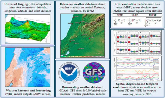
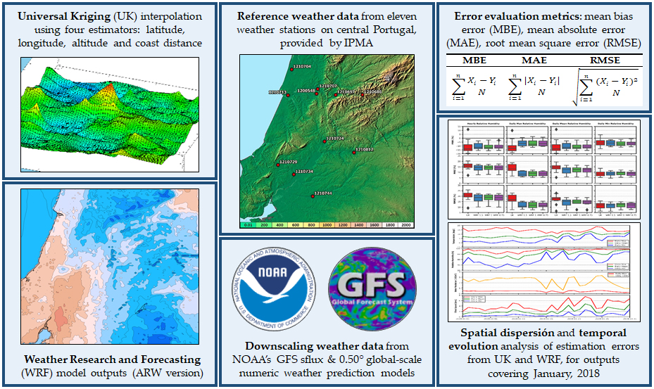
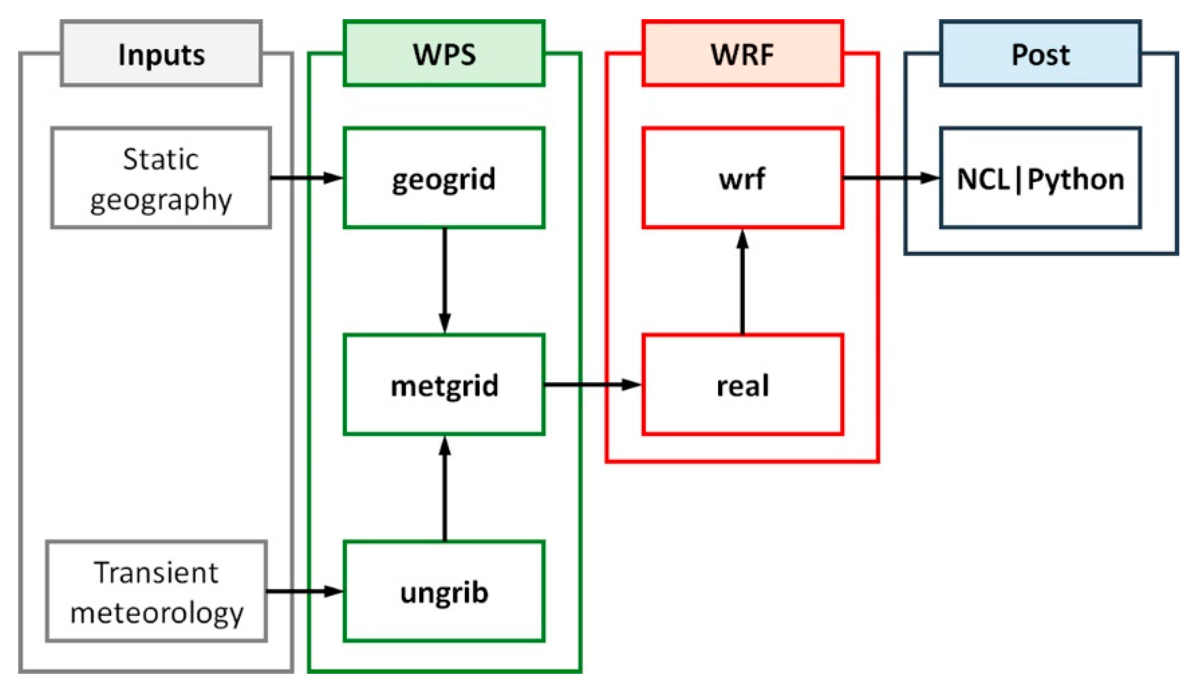
2.1. Downscaling Algorithms

The first chosen downscaling algorithm, belonging to the geostatistical interpolation tools field, is one member of the Kriging interpolation family. In particular, the Universal Kriging method is chosen, as it is a tool with which the authors have an extensive experience embodied on different published research works [21,22,23]. The Kriging term designates a set of geostatistical interpolation tools, of which Universal Kriging is one particular version. Given an unknown variable, all Kriging methods focus on estimating its local value at a given location (estimation point), based on local measurements on its surroundings (observation points). Relations between locations are based on the distance between each pair of points. Hence, Kriging interpolation is based on the assumption of autocorrelation between different measurements of the estimated variable. Said variable is usually a continuous field, although some variants make use of categorical fields. Kriging methods take their collective name from the geology and mining works of Krige [24], developed and formalised by Matheron [25]. Since then, Kriging has been adopted and widely used in other fields, such as radioactivity monitoring [26], building energy performance analysis [27] or meteorological data generation [28].
Depending on the assumptions about the statistical properties of the interpolated variable, (namely its general trend) different versions of Kriging are available. A more detailed explanation about said versions can be found in [19]. On this study, the chosen Kriging variant is Universal Kriging, using four predictors to estimate general trend: latitude, longitude, elevation taken from the mean sea level and horizontal distance taken from the nearest sea-land interface. Specialised R packages are used to build the implemented UK interpolation algorithm, including the definition of estimation and observation sets of points with defined predictors, the downloading of input weather data, the proper interpolation and the generation of output files.
The Weather Research and Forecasting model is one mesoscale NWP model widely used in conjunction with GFS, with a few examples being [9,10,12,13]. The Advanced Research WRF (ARW) [29] core version of WRF is maintained by the National Centre for Atmospheric Research (NCAR), and is mainly used for research studies. The other available core is the WRF Non hydrostatic Mesoscale Model (NMM), maintained by the National Centres for Environmental Prediction (NCEP). Some of the main differences between the ARW and NMM cores are their vertical levels systems, time integration methods, grid point conventions and conserved variables. In this study, version 4.1.1 of the ARW core is used. Hereinafter, the ARW core will be referred to as simply WRF, as the NMM core will no longer be mentioned.
A general outline of the WRF algorithm workflow can be seen in Figure 1. It can be divided in three main systems: the input data pre-processing modules (collectively referred to as the WRF Pre-processing System or WPS), the solver modules (the actual WRF model) and the post-processing and visualisation modules, along with other components not used on this study. More details about the WPS and WRF operation and underlying principles can be found on [30].
Default physic options for the 4.1 version are used on this study [30]. A hybrid vertical coordinate system is used: the bottom vertical layers follow the surface terrain, evolving into layers entirely defined by isobaric values for the top part of the atmosphere. WRF output files are processed using custom Python and NCAR Command Language scripts. Point measurements are extracted from the gridded result files at specific locations, retrieving meteorological values from the nearest grid point. Other python scripts are used to define WPS and WRF systems launch configuration, download input weather data, manage the general algorithm workflow and store intermediate outputs and log files.

2.2. Data Sources

Among the different input data required for both UK and WRF algorithms, the most relevant are observations of weather variables on a sufficient amount of points, which can be either real on-site measurements or reliable estimations obtained with other methods. For UK interpolations of a given variable, only two-dimensional (2D) inputs over a latitude-longitude defined grid are required for each interpolated moment, with the same elevation over the local ground surface. For WRF, however, a plethora of different weather variables are to be provided at a three-dimensional (3D) regular grid to properly model the regional atmospheric dynamics. These weather inputs provide the boundary and initial conditions for the atmospheric simulation. As any interpolation method has an intrinsic amount of error, a reference dataset of reliable measurements at a representative set of the estimated points is also required in order to measure the accuracy of the interpolated results.

2.2.1. Input Weather Data

The main weather data used in this study are two of the NOAA weather forecast products. Specifically, outputs from the Global Forecast System products GFS 0.5° (spatial horizontal resolution of 0.5°) and GFS sflux (horizontal resolution of ~13 km) are used as meteorological inputs for WRF and for UK algorithms, respectively.
The NOAA is one of the operational units belonging to the United States Department of Commerce. It is a scientific entity mandated to provide information and promote research focused on oceanic and atmospheric conditions. The NOAA’s Global Forecast System NWP model is developed and maintained by members of the NCEP. Various GFS products are available with alternative horizontal grid resolutions (among other differences). All GFS models have four daily executions at 00:00, 06:00, 12:00 and 18:00 UTC time, generating outputs up to 384 hours. Forecast output files have a temporal resolution of one hour for GFS 0.25 and sflux products for the first 120 hours, increasing to 3-hourly outputs beyond forecast hour 120 and up to forecast hour 384. For the GFS 0.5 and 1.0 products, the temporal resolution is three hours for all the forecast range. NOAA maintains a network of data servers inside the framework of the National Operational Model Archive and Distribution System (NOMADS) project. There, access is provided to both a long-term archive (file persistence lifespan of roughly two years) of some model outputs, and a short-term real time server (file persistence of 10 days) where all currently operated model outputs are published. For the long-term archive, only files containing results at every other three hours are available. More information about GFS products is available at [15,31].
For the current study, GFS 0.5° three-hour resolution outputs are retrieved from the long-term archive, and GFS sflux hourly results are downloaded from the short-term archive. Only the shortest possible term forecast files are considered for each cycle (e.g., the +03 forecast of the 06 execution cycle is used, instead of the +09 forecast of the 00 cycle). Both GFS 0.5° and sflux data are fed into the WRF and UK algorithms without any modifications to the values contained within the downloaded files. The only pre-processing of GFS sflux data is the extraction of relevant weather variables values for the points located inside the study area, as the UK algorithm is not capable of directly reading full GFS output files. For the GFS 0.5° files, they are directly ingested by the WPS module, without any external pre-processing. A detailed explanation about the WPS internal pre-processing operations can be found on [30].

2.2.2. Reference Weather Data

The reference institution for weather science in Portugal is the Instituto Português do Mar e da Atmosfera (IPMA), a public entity commissioned with promoting and coordinating scientific research and technologic development on both sea and atmosphere. Among other attributions, the IPMA holds the national authority role for the meteorological domain in Portugal.
IPMA maintains a network of 135 automatic weather stations over the continental and insular Portuguese territory, which yields an approximate density of one station per 667 square kilometres. For the central area of Portugal where this study is focused, 37 units are scattered along the districts of Coímbra, Castelo Branco, Leiria, Portalegre, Santarém and Lisboa. Almost all of them hold dry bulb air temperature, air relative humidity, global solar radiation, accumulated rainfall and mean wind sensors, with fewer measuring atmospheric pressure.
IPMA provides free access to the current weather conditions (only a few variables) over all the Portuguese territory on its web site. Historical data must be specifically requested, normally with a fee that depends on the amount of requested information. However, a sample dataset containing hourly measurements from 11 stations during a complete month is provided free of charge by IPMA, in the framework of the SAFEWAY project where this study is included.
Attempting to evaluate grid-output estimation algorithms using empirical measurements (such as weather stations) introduces a new issue: measurement points are prevalently scattered in an irregular pattern, with a lower point density on remote, unpopulated areas. Estimation algorithms such as WRF require defining a regular output grid, whose nodes coordinates may not match the irregular measurement locations. Trying to ensure this matching would usually require the estimation grid to have a spatial resolution close to the resolution used to define the measurement points coordinates, which is not feasible on most cases. To tackle this issue, most studies opt to fit point measurements into a regular, compatible grid using interpolation methods, such as Kriging [17,18,32]. Another option is to interpolate the estimation grid points to the measurement locations. The former approach introduces an artificial error level on the measurement reference dataset, while the latter increases the uncertainty of the estimation dataset. In this study, the latter option was chosen for WRF results, interpolating its estimations from WRF grid points to IPMA stations locations using a simple Nearest Neighbour method (i.e., assigning the value of the closest estimation grid point). A brief presentation of the distance errors between the IPMA measurement points and their nearest WRF estimation points is presented in the Section 2.4.

2.2.3. Auxiliary Data

Although weather observations are capital inputs for both downscaling algorithms, more data is required. For the UK algorithm, both latitude and longitude estimators are always known for well-defined observation and estimation points. Elevation from sea level and distance to nearest coast line, however, are not necessarily available when choosing estimation locations or when retrieving local weather measurements. These two required variables must be obtained from a digital elevation model and a geographic geometry model with enough spatial resolution, as they limit the resolution of the interpolation results. Here, altitude is measured using a public European elevation model provided by the European Environment Agency under the framework of the Copernicus programme [33], which has a 25 m resolution and a vertical accuracy of ±7 m RMSE (Root Mean Square Error). Coast distance is measured using a public European coastline dataset provided by the European Environment Agency [34], showing separation of land and sea at a 1:100,000 scale. Frontiers of inland water bodies that are not connected to sea are not included on this dataset.
For the WRF algorithm, static geographic data must be interpolated to the different model grids by the geogrid tool. These static data include soil categories, land use categories, terrain height, annual mean deep soil temperature, monthly vegetation fraction, monthly albedo, maximum snow albedo and slope categories [30]. For this study, the high resolution mandatory geographical data package provided in [35] is used. This is the standard geographical dataset used on operational WRF runs.

2.3. Study Operational Conditions

After selecting the downscaling algorithms and the input weather and auxiliary data sources, the specific conditions of the comparison test between UK and WRF must be defined. These are conditioned by the framework of this study, the SAFEWAY research project. Meteorological activities on said project are focused on the central Portugal region during years 2019-2021. This determines the relevant weather variables to be analysed, and restricts the geographic area and temporal interval of the study.

2.3.1. Studied Locations

Eleven locations across the Portuguese districts of Coimbra and Santarém were selected to perform the comparison between UK and WRF weather estimations. These locations correspond to the sites of the eleven IPMA automatic weather stations available on those districts, which were used to provide the reference weather data. Coordinates and relevant information about the chosen locations are shown in Table 1.

2.3.2. Temporal Span

Reference weather dataset provided by IPMA ranges from 1 January 2019, 00:00 to 31 January 2019, 23:00, with a resolution of one hour. The local GFS sflux results database fully covers this time span with hourly entries. For the GFS 0.5° files, the 18 cycle execution for 29 January 2019 is missing from the online NOMADS archive, as are all subsequent executions until the cycle 18 of 2 February 2019. This gap could be filled using longer-term forecast files from the last available execution. However, this would reduce the quality coherence between the sflux and 0.5° results. Instead, the last three days of January were removed from the analysed temporal range. Thus, the current study used hourly results from 1 January 2019, 00:00 to 28 January 2019, 23:00, both included. All hours mentioned thus far and henceforward are UTC.

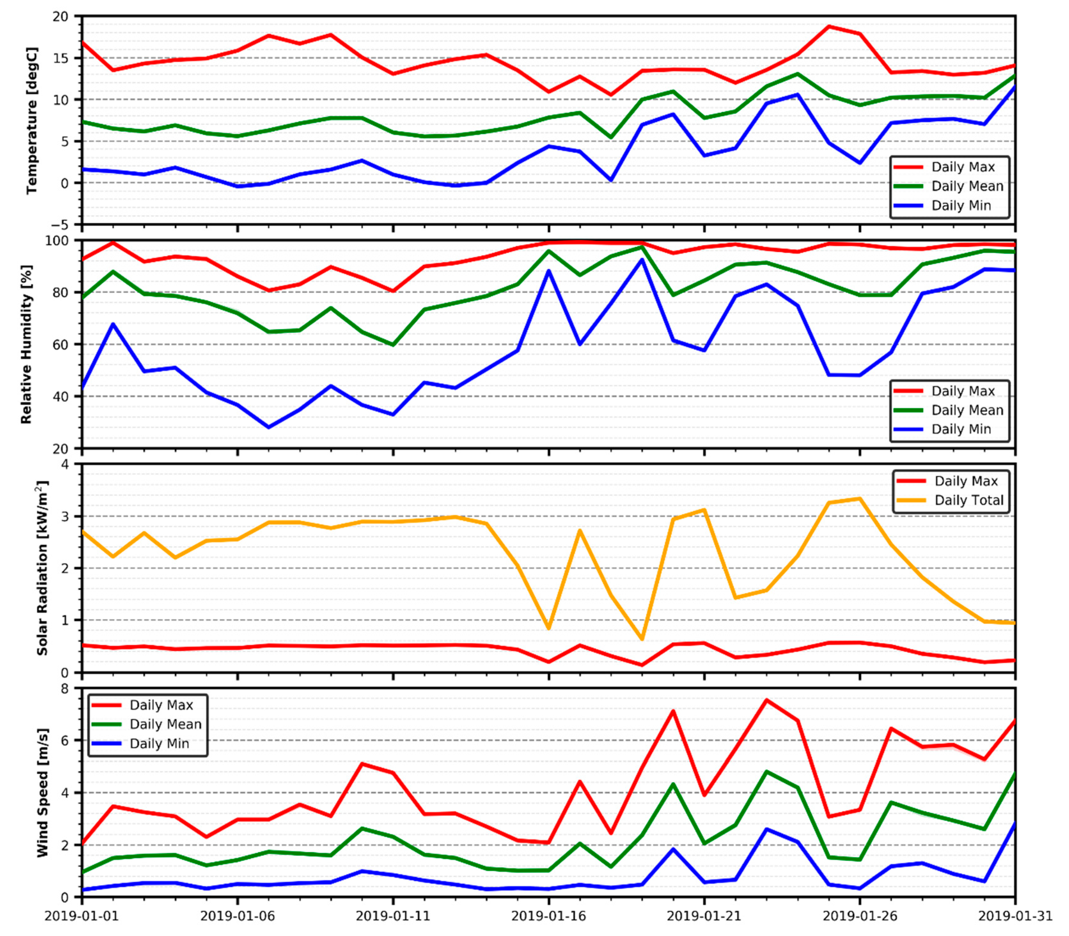
2.3.3. Weather Variables

Relevant weather variables for this study are selected based on three criteria: (i) the significance to fully characterise local atmospheric conditions; (ii) previous work from the authors regarding Kriging performance with meteorological data [21,22,23]; and (iii) the availability on the reference data acquired from the selected IPMA stations. According to the first two criteria, variables containing temperature, humidity, pressure, solar radiation, wind and rainfall information were selected. According to the last criterion, the analysis of pressure related variables is omitted due to such variables not being included on the provided reference datasets. Rainfall, although being a relevant weather variable as identified during the literature review, has to be discarded for this study. This is due to the small percentage of valid and not zero rainfall data available from the IPMA reference dataset: between the hours with no valid measurements, and the ones where the stations registered no rainy conditions, only a 11.9% of the total hours of the study span could be used to validate rainfall estimations. Wind direction is also discarded for a similar reason, having only a 24.9% of non-error measurement hours on the reference dataset. Wind speed, another relevant weather variable according to the literature review, was provided separately from wind direction on the reference dataset, and has a much higher percentage of valid measurements (77.7% of the total hours), thus, it was considered for this study.
The chosen variables are: air temperature, air relative humidity, global solar radiation and wind speed. With this set of variables, the study comprised a well-acknowledged relevant weather factor (wind speed) [4], a possibly relevant condition (air temperature) [3] and two not previously considered conditions (air humidity and solar radiation), which have nonetheless potential to alter road conditions. Temperature, humidity and wind speed variables are hourly mean averages, built from sub-hourly measurements or estimations. The solar radiation variable is an hourly total, integrated by sum of sub-hourly measurements or estimations. In addition to these hourly variables, more metrics based on daily aggregations of hourly values were also considered for the comparisons. Maximum, minimum and mean daily values were computed for temperature, humidity and wind speed. For global solar radiation, the minimum value is trivial. For this sole variable, the total daily amount of recorded radiation (a sum of hourly values) was used, in addition to the maximum daily value.
For the solar radiation variables, a filter was applied when computing errors between estimated and measured values in order to only consider hourly data between 07:00 and 19:00 (both included). Thus, the night radiation values are excluded from the calculations, since they ought to be zero for all estimated and measured datasets. The 07:00 and 19:00 limits are chosen after analysing the IPMA radiation measurements, to ensure that the compared hours comprise both dawn and dusk hours for all stations and days.

2.4. Compared Datasets

Four different datasets of estimation results were generated for comparing the performance between the UK and WRF algorithms, based on the achieved horizontal resolution. Three different datasets are built for the latter, all using GFS 0.5° files as weather data inputs. Only one dataset was built for the former, with the GFS sflux local database stored variables used as inputs.
For Kriging interpolation, it makes no sense to state an output spatial resolution, since UK results are not inherently limited to a specific discrete grid. Auxiliary data inputs, however, do have a spatial horizontal resolution of 25 m. Although it does not directly translate into an output resolution, said input resolution does have an influence on output errors.
For the WRF algorithm, a horizontal resolution must be defined for each of the nested interpolation meshes. In this study, a three nested meshes structure is defined for an adequate transition between the roughly 56 (north-south) – 39 (east-west) km resolution of the GFS 0.5° grid and the innermost output mesh. For each of these meshes, three different resolution options were tested, keeping a constant resolution ratio of 3 for each subsequent nesting (4 for the third set). A two-way nesting approach was used, thus, each nested mesh overwrites results of its parent mesh on the overlapped area. Meshes coordinates and resolutions are shown in Table 2, while UK estimation point locations (including related IPMA station codes) and WRF interpolation meshes can be seen in Figure 2.
Once both WRF estimation grids and IPMA reference points were well defined, distances between each measurement location and its nearest WRF estimation grid point were computed. These distances provide an indirect form of evaluating the error introduced when translating the reference locations to the estimation grid, as a direct estimation of said error was not possible due to not having local data measured on the exact grid points. Distances for the three different WRF meshes sets can be seen in Table 3. The maximum possible difference between estimation and measurement points would correspond to half of the diagonal size of a rectangle defined by the surrounding estimation grid points. Mean distances for the 11 locations were between 50.3% and 61.9% of this theoretical maximum.

2.5. Error Comparison Metrics

Estimated datasets quality is tested using different error metrics to evaluate deviations from the reference IPMA stations measurements. Based on previous studies carried out by some of the authors [21,22,23], three error metrics are chosen: the mean bias error (MBE), mean absolute error (MAE) and root mean square error (RMSE), whose definitions are shown in Table 4.

3. Results and Discussion

Differences between the reference IPMA dataset and the Kriging and WRF datasets are analysed by means of the three aforementioned error metrics, and results are presented using two different methods: first, the spatial variability between estimations performance on the 11 selected locations is explored using box-and-whisker plots; second, the evolution of the error performance during the study temporal span is studied using line plots. In addition, an analysis of the IPMA measured data is also included before the main results to check the general weather conditions.

3.1. Reference Ranges

A first look at the daily maximum, mean and minimum values of the IPMA dataset for each variable is provided in Figure 3, in order to identify the general weather conditions. This helps providing reference ranges of values, so differences between different error metrics can be properly evaluated. For global solar radiation, the minimum value is replaced with the total daily amount of radiation obtained.
Weather daily values show that the first 13 days are slightly colder, sunnier and with lower winds and more stable conditions than the rest of the study time span. Weather conditions fluctuations are high but not extreme, with a maximum difference between higher and lower temperatures of 16 °C for a given day between all locations. Mean temperature, humidity and wind speed values present a moderately cold, humid time period with weak winds. These values will be useful in the evaluation of metric error magnitudes on the following sections.

3.2. Spatial Dispersion Analysis

Box-and-whisker plots represent the mean estimation results variability for the eleven tested locations for each UK or WRF dataset. Median or 50th percentile (horizontal line inside boxes), 25th and 75th percentiles (bottom and top box closures) and differences between those two percentiles (inter-quartile range) are analysed and compared. All three 25th, 50th and 75th percentiles may be referred to as the main percentiles hereinafter. On the following figures, whiskers comprise values outside of the inter-quartile range but within 1.5 times such range. Outliers falling outside of whiskers are marked as black rhombuses.
MBE, MAE and RMSE results are plotted for each hourly variable and its related daily aggregations. As shown in Figure 4, all datasets tend to overestimate the temperature in all of its forms, although MBE values are much closer to zero for the daily maximum aggregation. The UK interpolation 25th percentile value is the lowest in all but the maximum temperature cases. Median, 75th percentile and inter-quartile range values are the highest for the UK dataset in the four temperature aggregations. Differences are less prominent between WRF datasets than between them and the UK results. WRF-1 has a slightly better performance than WRF-1.5 and WRF-0.75 regarding inter-quartile and 75th percentile values, while having higher 25th percentiles and similar medians.
Relative performances are similar for MAE and RMSE metrics. UK dataset now has higher main percentiles and median values, but its inter-quartile ranges are smaller than the ones of the other datasets. As for the WRF outputs, WRF-1 has again a smaller inter-quartile range but a slightly larger distance between top and bottom whiskers, while median values are similar in the three datasets.
While hourly and daily mean temperatures behave very similarly, maximum and minimum temperatures have large discrepancies in performance: main percentiles and median values are between two and five times higher for the minimum temperatures, while inter-quartile ranges differences can reach up to 26 times for the case of WRF-1.5. Maximum and minimum daily temperatures taken from Figure 3 help to evaluate the magnitude of the obtained errors: having a RMSE of ~1 °C (median values for the four estimation datasets) for the highest daily temperatures in the range of 20 °C is less significant than the RMSE of 3–5 °C for lowest daily temperatures, close to 0 °C for most of the days. Comparing maximum and minimum temperatures metrics, the hours with colder temperatures seem to produce the largest errors.
Overall, WRF datasets perform better than the UK one for the temperature variables, although differences vary between metrics and aggregations. Based on median, main percentiles and inter-quartile range values, the best temperature estimations are provided by WRF-1, with WRF-1.5 and WRF-0.75 being technically tied on the second position, close to first.
MBE results from Figure 5 reveal the global tendency of all estimation datasets to underestimate relative humidity. As with temperature, differences between humidity WRF-1 and WRF-0.75 datasets are smaller than when comparing them against the UK results. However, the WRF-1.5 results performance is now more separated from the other WRF datasets, especially for inter-quartile ranges and 75th percentiles. Medians are similar for the three WRF outputs, and also for UK for the daily minimum values.
Performance patterns are again similar between MAE and RMSE, also showing the same trend as MBE: UK performing notably worse than WRF-1.5, WRF-0.75 and WRF-1 (ranked in that same decreasing order of performance) for hourly values and the two first daily aggregations, while differences are much less obvious for daily minimum humidity values. While all WRF datasets have similar values for medians and 75th percentiles, the 25th percentile values are higher for the medium resolution one, meaning less estimation values have a lower error for this dataset.
Although differences between maximum and minimum humidity errors do exist, they are not as significant as for temperature. The largest variations appear between daily mean and minimum metrics for the WRF-0.75 dataset. Taking into account the mean humidity measured values of 70–90% for most days from Figure 3, the median RMSE values of about 15% obtained are relatively high. RMSE errors are similar between maximum and minimum daily values for all the WRF datasets (about 12.5%), but the latter are more relevant when compared to the measured high and low humidity values (40–70% for most days for the minimums, 80–100% for all days for the maximums).
UK dataset estimations show the worse general performance when all aggregations and metrics are taken into account. WRF-0.75 is arguably better than WRF-1 for daily minimum errors, while it is worse for daily minimums, yielding a comparable performance for hourly and daily maximums and mean values. As with temperature, there is no clear best dataset for the humidity variables. However, both WRF-1.5 and WRF-0.75 have arguably better performance than the medium resolution dataset.
Unlike temperature and humidity variables, Figure 6 shows a marked distinction between UK and WRF performance regarding solar radiation bias errors. While all three WRF datasets have a clear tendency to overestimate hourly and daily radiation, UK estimations show negative MBE median values, although they are closer to zero than the WRF datasets. WRF-1 has better 25th percentile value for daily highest radiation results and worse for hourly and daily totals. Differences are smaller between WRF-1.5 and WRF-0.75, with WRF-1 having a slightly worse performance.
For MAE and RMSE, hourly radiation performance variations WERE smaller than the ones showed for MBE, with the best performance median-wise being achieved by WRF-1 for MAE, and by UK for RMSE. Variations WERE larger for the daily maximum radiation results, where UK had the lowest median and 25th percentile but the highest inter-quartile range values. WRF-0.75 had the best performance for the three WRF datasets in all error results. For the daily total radiation, variations between datasets were lower, closer to the ones achieved for hourly radiation.
The daily sum of solar radiation is not directly comparable to the other two radiation variables. Comparing hourly and daily maximum results, the latter variable had a worse overall performance, especially for the UK dataset inter-quartile ranges, which doubled their values. Variability between datasets also increased when comparing those two variables. Nevertheless, even the worst median error value (daily maximum radiation of ~0.095 kW/m2 RMSE for WRF-1) was only 20% of the daily maximum measured radiation, ~0.5 kW/m2 for most days as taken from Figure 3. For the daily total radiation, reference values were 2–3 kW/m2 for most of the month, with the lowest achieved value being 0.6 kW/m2. Compared to these values, the median errors of less than 0.5 kW/m2 for all metrics were also less significant.
Results for solar radiation variables showed many differences when compared to temperature and relative humidity, and this was also true when choosing the best and worst overall performance datasets. In this case, the UK estimations outperformed the results from the three WRF datasets, while WRF-0.75 showed better results than its coarser counterparts.
Wind speed estimations shown in Figure 7 followed the same pattern as with temperature and humidity in regard to MBE results: the four compared datasets shared the common trait of overestimating both hourly wind speed results and its daily aggregations. The lesser bias was achieved by UK median results for the four wind speed variables, although its 75th percentile value was higher than the WRF datasets for the daily minimum results. Differences between UK and WRF datasets were much less pronounced for that same aggregation variable. Median and inter-quartile range MBE values were similar between WRF datasets.
MAE and RMSE results show the same general pattern as MBE, with UK performing notably better in all but daily minimums. Median values were again similar for all WRF datasets. The most remarkable difference with bias errors was that UK inter-quartile ranges were more similar to the WRF ones in both hourly and daily mean and minimum results.
Variability between different wind speed aggregations was not salient. The largest differences were between daily maximums and the rest of speed variables, but they were not as notable as with minimum temperatures or maximum solar radiation. All datasets performances were more similar for hourly and daily mean speeds, and also for the other two variables for the UK dataset. Reference measured values of 3–6, 1–4 and 0.5–1.5 m/s for maximum, mean and minimum speeds can be assumed for the most days (taken from Figure 3), despite the large variability for the second half of the month. Taking this into account, it can be stated that UK has a worse performance with weak winds, as the achieved median minimum speed values around ~1 m/s RMSE are more relevant than the ~1.2 m/s RMSE maximum speed values when compared to their respective reference values. The same cannot be as clearly stated for WRF datasets, as their median maximum wind values are larger (about 2.5 m/s RMSE) and hence more significant.
Overall, UK wind speed estimations achieved the best scores for the analysed results, surpassing its WRF counterparts performance for all wind metrics on hourly and daily maximum and mean values. Although it had the worst performance for daily minimum wind speed, its performance in that variable was close to the WRF datasets. No WRF dataset performed substantially better than others in all wind variables.

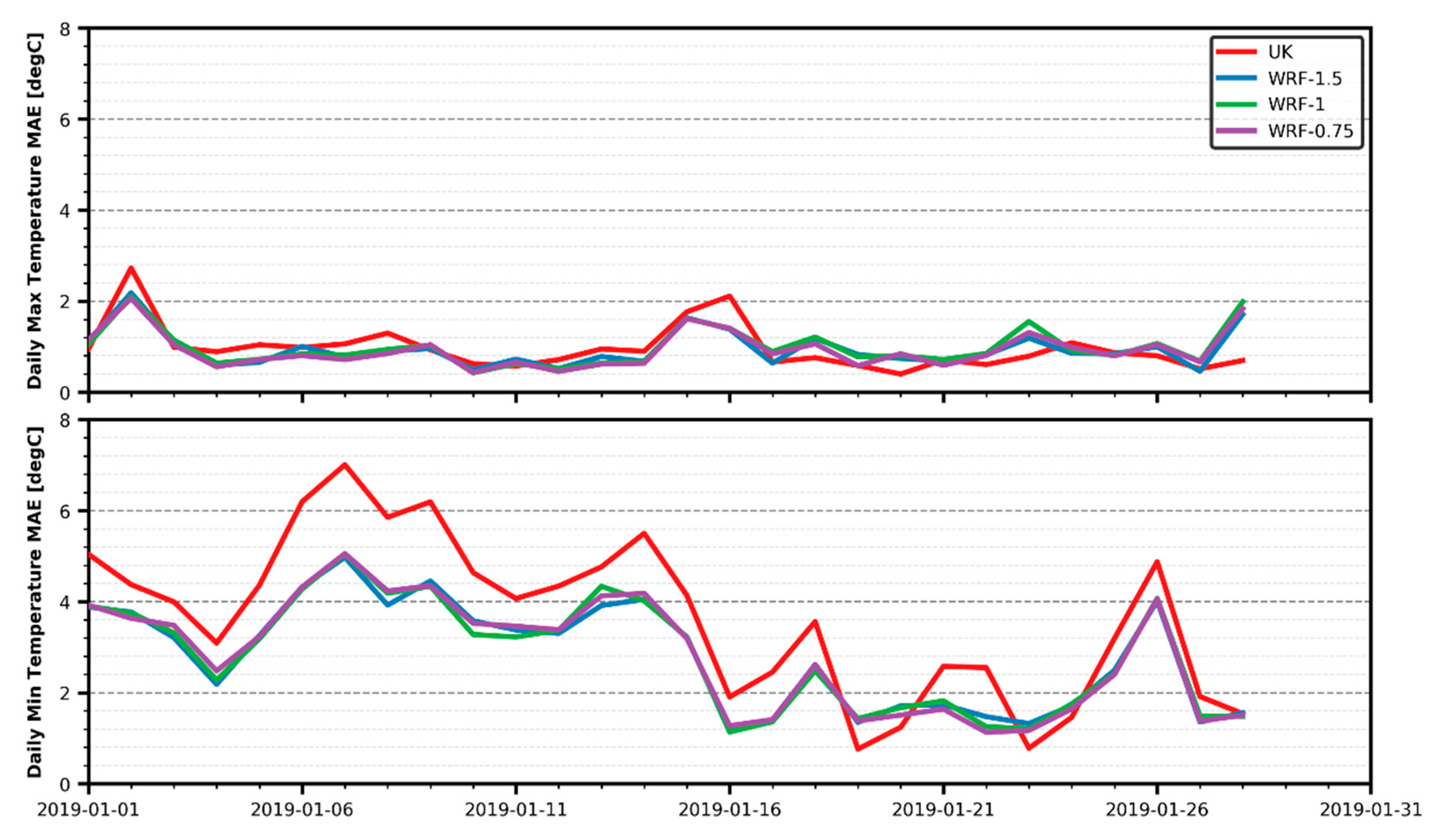
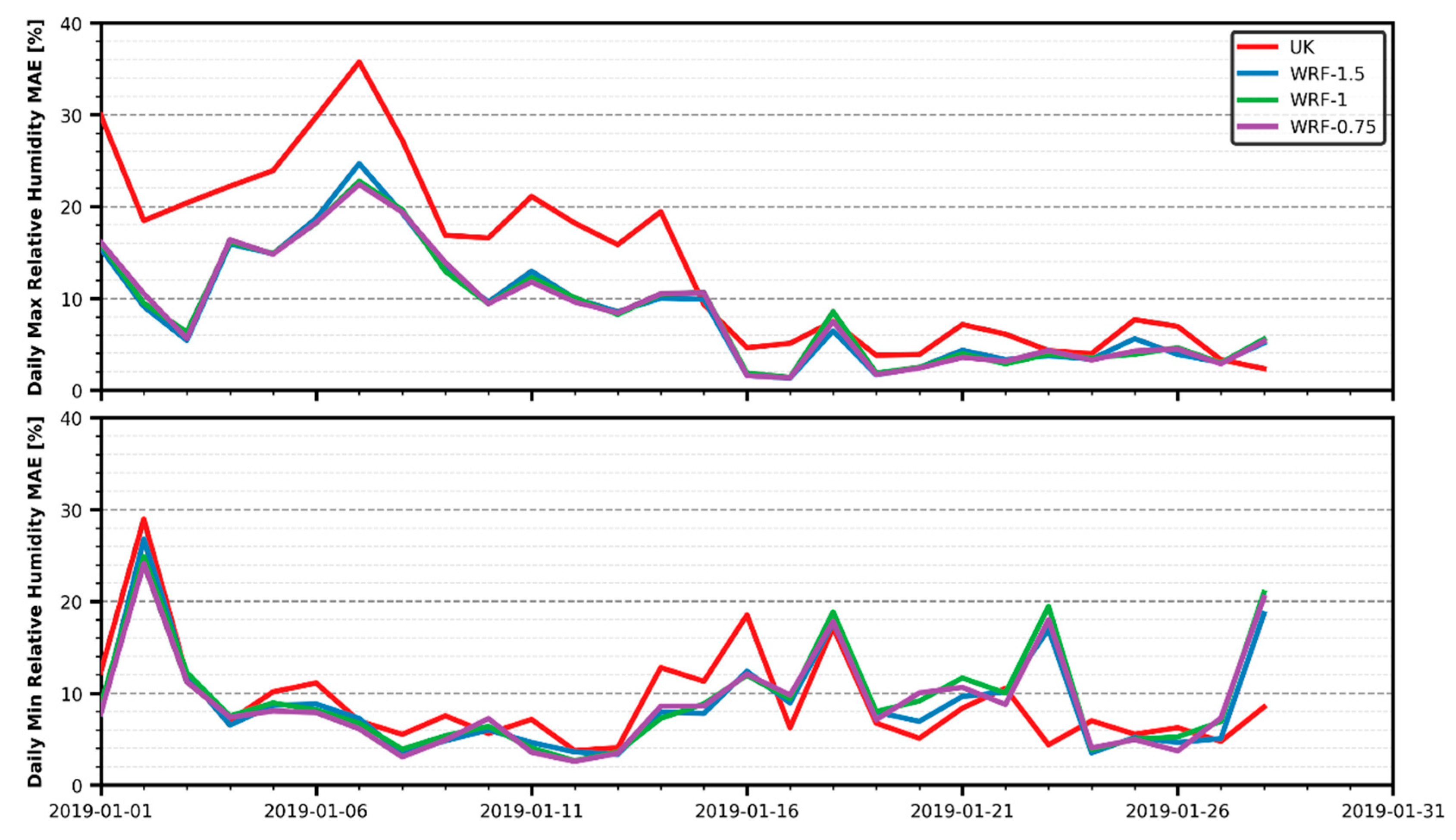
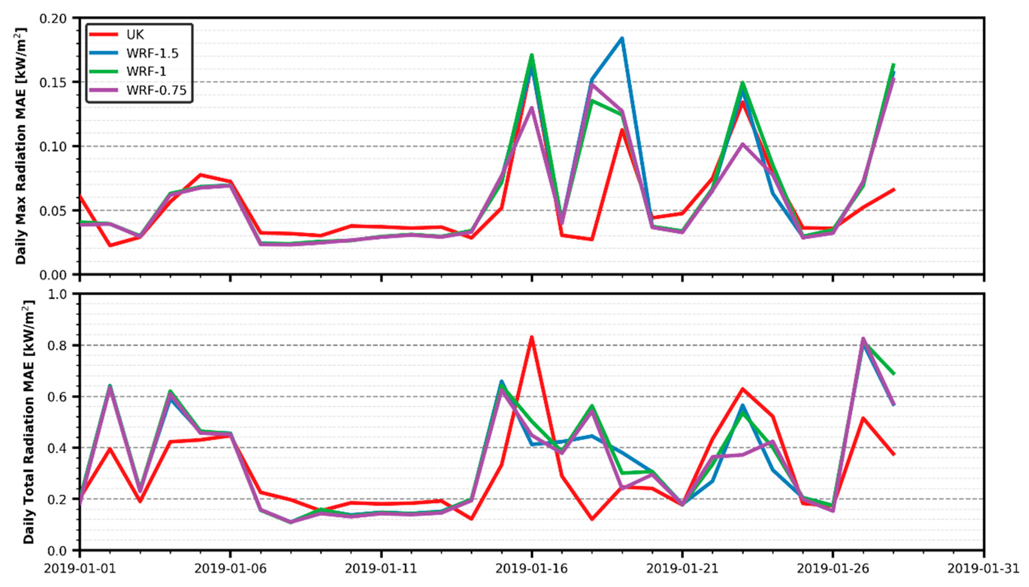
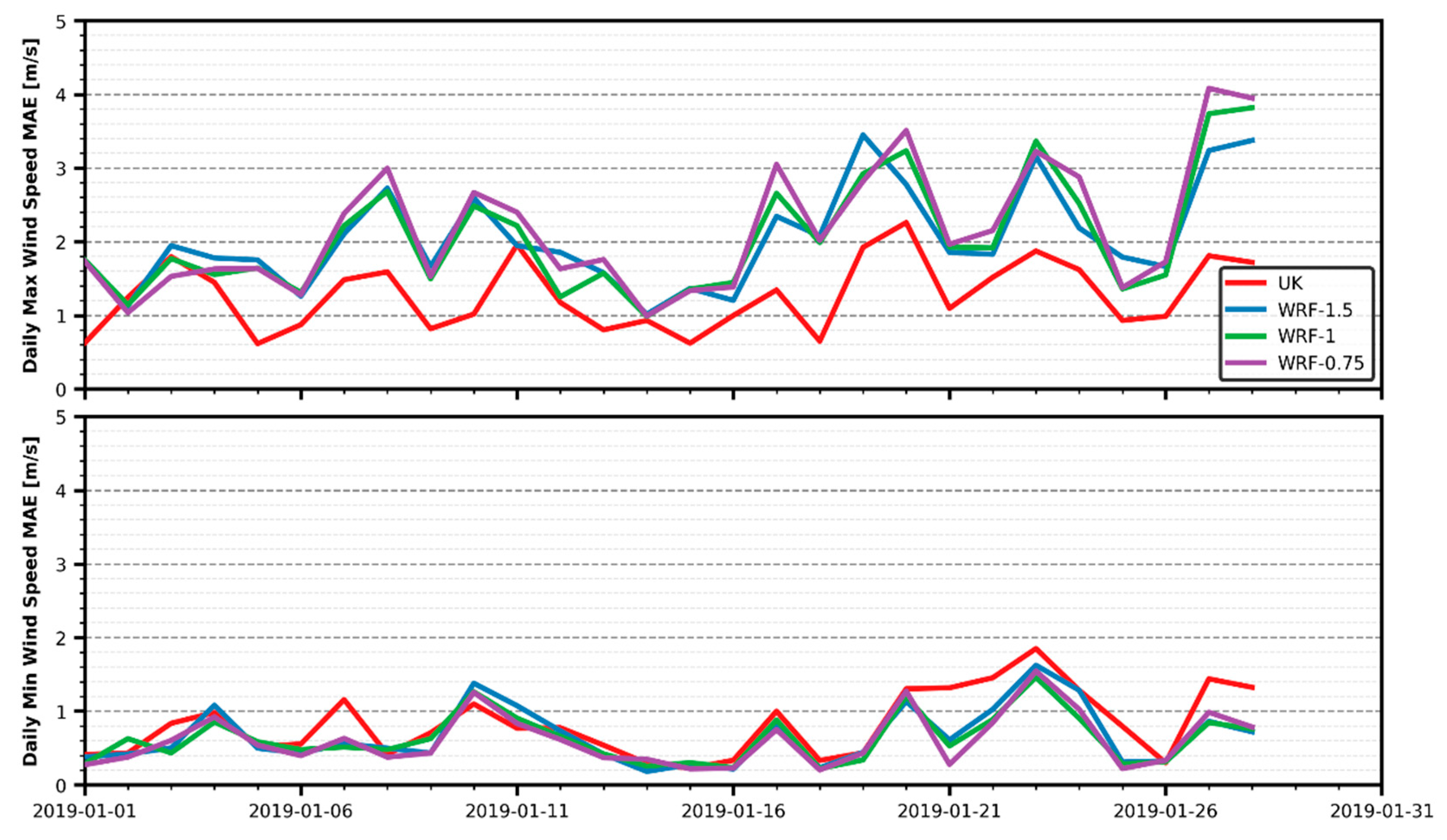
3.3. Temporal Evolution Analysis

MAE and RMSE results for each day are represented using line plots for daily maximum and minimum daily values of each variable (maximum and total values for solar radiation). Plotted errors are the averaged values of the 11 locations. This allows to study error performance evolution over the study temporal span. As plots for both metrics show the same general trends, only the former are presented.
Temperature errors daily evolution shown in Figure 8 reflect that minimum temperature MAE results have higher oscillations than the maximum ones. While the latter is almost flat for most days, the former has variations up to 4 °C within a few days. This is a notable fluctuation, compared to the reference minimum 0–5 °C measured for most days.
When comparing with reference values from Figure 3, a remarkable feature appears: for the second half of the analysed period, local maximums in MAE minimum temperatures matched local minimums in reference to low temperatures. This pattern was not present for the first 14 days, when reference minimum temperatures were consistently low but MAE values had significant fluctuations. However, it is true that for those days of consistently low temperatures, MAE errors were mostly high (in fact, this is the time period with highest errors). This seems to reinforce the idea that both UK and WRF datasets have problems estimating colder temperatures.
Overall, WRF datasets have consistently ~1 °C less error than UK for most days on minimum values, with almost negligible differences between WRF datasets. For daily maximum temperatures, UK performed much alike the other datasets, with differences lower than 0.2 °C, except for the last day with data. These are the same general patterns already commented on in Figure 4.
Figure 9 shows MAE results for daily maximum and minimum relative humidity. Mean daily maximums were higher for the first half of the month, with oscillations of a greater magnitude (up to 12% humidity variation between two consecutive days). For daily minimums, the trend was almost the opposite, with lower, more regular error values during the first 13 days (except for January 2nd, when all four datasets achieve the greatest error values). The greatest variation between two consecutive days was achieved for the first two days, where WRF datasets had a fluctuation of almost 20% of relative humidity).
A clear pattern relating local maximums on error and reference values evolution figures cannot be found here, unlike temperature. Peak error values achieved on January 2nd (all datasets), 16th (UK only) and 23th (WRF only) do match with local maximums on minimum relative humidity reference values, but this is not the case for the rest of spikes. No pattern can be found for daily maximum humidity.
The UK dataset performed much worse than WRF for daily maximum humidity results, while being much closer for daily minimums. As for temperature, differences between WRF datasets were almost negligible for most days, for both maximum and minimum daily results. The UK dataset had daily maximum errors near 10% greater for the first half of the month, and less than 4% for the second half. For daily minimum relative humidity, those differences were less than 5% for all but four days. This reinforces the results already commented in Figure 5.
Both daily maximum and daily total solar radiation error temporal development shown in Figure 10 follow the same general pattern. After two wide oscillations during the first week, another seven days of regular, low errors follow. The second half of the analysed month features the larger fluctuations for all datasets. WRF-1.5 achieves the global largest oscillation between January 19th and 20th with 0.14 kW/m2 for daily maximum radiation. For daily totals, all three WRF datasets achieve a ~0.6 kW/m2 difference between January 26th and 27th.
For all significantly reductions in daily total radiation reference values (already shown in Figure 3), a notable increase in WRF MAE errors arose. The same pattern was followed by UK estimations, except for January 17th, where its mean error fell rather than growing. Daily maximum radiation oscillations also occurred on the same days as daily totals (less marked due to the different natures of both variables), and were also translated into oscillations on the MAE results. However, the magnitude of the oscillation on the reference values does not seem to directly reflect on the magnitude of the MAE result oscillation. This can be clearly appreciated when comparing daily total oscillations on the first days with the ones occurring during the second half of the month.
Divergences between datasets were steep during days with strong oscillations, and less significant during periods with more regular error results. None of them showed a consistent good performance during all those swings. Radiation estimations from the three WRF datasets had more deviations than those of temperature and humidity during the strong oscillations in the second half of the month. For daily maximum radiation, differences between estimations ranged from ~0.01 kW/m2 during the days surrounding January 11th to almost 0.1 kW/m2 on January 28th. Equivalent dissimilarities could be found during some days for daily total radiation. Overall, UK can be chosen as the better estimator of daily maximum solar radiation, while its first ranking for daily total radiation is more debatable. This is not unlike the MAE results already shown in Figure 6.
Variability between days was high for all datasets on both daily maximum and minimum wind speeds, according to Figure 11. For the former, inter-daily oscillations can be up to 2 m/s between two consecutive days, and ~1 m/s for the latter. When compared to the reference values of 3–5 m/s (daily maximums) and 0.5–1.5 m/s (daily minimums), error fluctuations on both variables were significant.
For daily minimum wind speed, error oscillations between January 19th and January 28th seemed to follow the same pattern as reference minimum values fluctuations. However, the relatively plain reference values for the first 18 days do not account for the variability in error results, similar in magnitude to the latter days. For daily maximum speeds, strong oscillations were present during all month on both reference values and error results. They seem to follow the same general pattern, increasing and decreasing errors when reference values did so. However, there was no proportionality between errors and measured values fluctuations, as the larger swings during late January and smaller variations during early January for the latter seem to cause error oscillations of a similar magnitude. It should be noted that UK errors magnitudes were more alike than for WRF when comparing daily maximum and minimum MAE results. As reference values for minimum wind speeds were notably lower than the maximum speed ones, it can be concluded that UK estimations were worse for winds of low speed.
UK estimations have the best performance on daily maximum wind speed results for all days, except for three dates when it is tied with WRF. UK errors were between 0.2 and 1 m/s lower than the WRF ones for most days, while differences between WRF datasets were only larger than 0.4 m/s for 6 days. For the daily minimum speeds, UK errors are significantly higher for five days (around 0.75 m/s), and similar for the rest of the month. Greatest variation between WRF estimations for the same day is only of 0.4 m/s. These behaviours are congruent with the results already shown in Figure 7.

3.4. Further Considerations

In this closing subsection, two notes regarding limitations of this study and computational performance of the used algorithms are included, which are not directly related to the results already presented and would cause the following conclusions section to grow exceedingly. However, the authors consider that both items provide relevant information that may help determining relevant future research directions.
As already stated, this study is limited by its spatial and temporal boundaries: only a mid-winter month of reference data is available for eleven locations of similar geographical characteristics (low or mid-low altitudes, relatively close to open ocean, all of them detached not more than 170 km). A further study should check the existence of systematic estimation biases, discard hidden local weather features and verify the general performance of the different downscaling methods. For this, a wider study area with more different geographical features should be analysed. Additionally, a larger temporal span with more variability on general weather conditions should be chosen. Both the spatial and temporal boundaries of such analysis would be limited by the availability of sufficient weather data measured from weather stations, which also constrains the applicability of this research study. However, results and conclusions exposed here do apply to the studied general weather conditions, namely, moderately cold, humid winter days with weak winds.
The present study was focused on evaluating the performance of two different downscaling tools, based on comparisons against measured local data and computation of error metrics. Hence, the selection of the best tool was based exclusively on those error metrics. However, when working with this kind of tools, the computational time needed for generating estimation outputs is a key factor on the production stage. The UK interpolation algorithm used here takes a given amount of measured or estimated weather data, and generates a single local estimation. It is time-independent, which means only global or regional weather data for a given temporal instant is required for obtaining a local estimation at that given instant. It is also output-independent, which means an estimation at a chosen location is generated each time, without requiring the computation of estimations on the surrounding area. The WRF tool, however, generates a grid of points where local estimations are computed. It is time-dependent, as interpolated outputs for a given instant are developed as an evolution of outputs for a previous instant. Unlike UK, it is output-dependent. This means it is not reasonable (although possible) to use this algorithm to generate estimations over a single local point, as a minimum estimation grid area is required to generate meaningful outputs.
The used Kriging algorithm, in its current form, is more than one order of magnitude faster than its WRF counterpart when estimating a single local datum at a single temporal instant. When working with a large enough area, the WRF algorithm beats UK in regard to time performance. The selection of the most adequate tool is thus dependent on the specific study area. Moreover, no strong optimisations are introduced on the implementation of neither the Kriging nor the WRF algorithms used. All these considerations are left out of the scope of this study, as they do not affect the error-wise quality of the obtained estimations, and they would require a totally different set of analysis not related with the ones chosen here. However, further optimisation research on both algorithms regarding computational performance is being considered, thus, their applicability to production level projects can be enhanced.

4. Conclusions

This study presents an evaluation of the estimation performance for two global-to-local weather data downscaling algorithms based on the Weather Research and Forecasting Model and Universal Kriging, two of the leading exponents of their respective fields (Numerical Weather Prediction models and geostatistical interpolation tools, respectively). Four weather variables were estimated using three different WRF grid configurations and one UK setting. UK and WRF tools were fed with similar global scale input weather data, based on the Global Forecast System model outputs. However, the GFS sflux model used for Kriging interpolations had a denser grid of calculated points than the GFS 0.5 model compatible with WRF. Results were compared against local measurements from 11 weather stations located on the central area of continental Portugal during the first month of 2019. Spatial and temporal distribution of three different error metrics were analysed.
As already stated in the results section, the rather short experimental campaign of reference measurements caused almost all analysed hours to have similar weather conditions, limiting the generalisation of extracted conclusions. This issue was further fostered by the small variability on geographic and orographic characteristics of the measurement locations. A future research work using data from different time periods would help in reassuring or modulating said conclusions.
Results show that the WRF datasets overestimated temperature, solar radiation and wind speed values, and underestimated relative humidity. UK estimations were positively biased for temperature and wind speed, while being negative biased for relative humidity and solar radiation. Considering this, algorithms could be adjusted to compensate a potentially systematic bias. Of the analysed weather variables, air temperature and relative humidity had a clear, physical inverse relation: relative humidity values will decrease for an increase in temperatures, provided that atmospheric pressure and water vapour species concentration are maintained. As all estimated datasets presented a clear overestimation of temperature values, an underestimation of the relative humidity results is to be expected. Of course, this behaviour could be influenced by non-adequate estimations of atmospheric pressure or water species concentration, not analysed in this study.
UK had the best performance estimating solar radiation and wind speed, and the worst for temperature and relative humidity. Amongst the WRF datasets, the 0.75 km spaced grid managed to achieve the best performance for solar radiation; however, for temperature, humidity and wind speed results, the differences were less remarkable. Overall, it was not possible to choose a WRF mesh resolution setting that consistently provided the best results for all four analysed variables, although differences were almost negligible in all but solar radiation.
Both the UK and the three WRF datasets produced worse estimations for minimum daily temperatures, and seemed to have a more irregular, overall worse performance with lower temperatures. All datasets achieved a lower accuracy on solar radiation estimations during overcast, less sunny days. For the UK dataset only, weak winds seem to be relatively worse estimated than strong ones. These patterns could be related to the relative clustering of the test locations: local geographical features could be causing deviations in local weather, which the global GFS models (which fed both UK and WRF tools) might not be able to capture. If this was the case, a finer tuning of the parameters of the algorithms would be required.
This study shows that access to local measured data is not an imperative requirement for generating local weather estimations, having (at least) two different valid options regarding the downscaling algorithms. A valid methodology for this global-to-local weather data downscaling was tested, with satisfactory results. It also highlights the different performances of weather downscaling tools depending on the nature of the interpolated variable. Overall, this study presents an initial step towards the selection of appropriate global/regional-to-local downscaling tools for mapping of weather conditions.

Author Contributions

Conceptualisation, J.L.G., F.T.P. and P.E.O.; Data curation, J.L.G.; Formal analysis, J.L.G. and F.T.P.; Funding acquisition, E.G.Á.; Investigation, J.L.G.; Methodology, J.L.G.; Project administration, E.G.Á.; Resources, E.G.Á. and P.E.O.; Software, J.L.G. and F.T.P.; Supervision, P.E.O.; Validation, J.L.G. and F.T.P.; Visualisation, J.L.G. and P.E.O.; Writing—Original draft, J.L.G.; Writing—Review and editing, F.T.P., E.G.Á. and P.E.O. All authors have read and agreed to the published version of the manuscript.

Funding

This investigation article was partially supported by the University of Vigo through the grant Convocatoria de Axudas á Investigación 2018: Axudas Predoutorais UVigo 2018 (grant number 00VI 131H 641.02). This investigation article was also partially supported by the Galician Government by means of the Xunta de Galicia CONECTA PEME 2018 (Project: TOPACIO IN852A 2018/37). This paper was carried out in the framework of the GIS-Based Infrastructure Management System for Optimized Response to Extreme Events of Terrestrial Transport Networks (SAFEWAY) project, which has received funding from the European Union’s Horizon 2020 research and innovation programme under grant agreement No. 769255. Neither the Innovation and Networks Executive Agency (INEA) nor the European Commission is in any way responsible for any use that may be made of the information it contains.

Acknowledgments

The authors would like to thank to the National Oceanic and Atmospheric Administration (NOAA) for providing public, free of charge access to both their real-time and historic GFS models output files.

Conflicts of Interest

The authors declare no conflict of interest.

Abbreviations

The following abbreviations were used in this manuscript.
ARWAdvanced Research WRF
ECMWFEuropean Centre for Medium-Range Weather Forecasts
GFSGlobal Forecast System
IFSIntegrated Forecast System
IPMAPortuguese Meteorological Agency (Instituto Português do Mar e da Atmosfera)
MAEMean Absolute Error
MBEMean Bias Error
NCARNational Centre for Atmospheric Research
NCEPNational Centres for Environmental Prediction
NMMNon hydrostatic Mesoscale Model
NOAANational Oceanic and Atmospheric Administration
NOMADSNational Oceanic and Atmospheric Administration Operational Model Archive and Distribution System
NWPNumerical Weather Prediction
RMSERoot Mean Square Error
UKUniversal Kriging
WPSWRF Pre-processing System
WRFWeather Research and Forecasting
WRF-1.5WRF dataset using a 1.5 km spaced innermost mesh
WRF-1WRF dataset using a 1 km spaced innermost mesh
WRF-0.75WRF dataset using a 0.75 km spaced innermost mesh

References

  1. Saha, S.; Schramm, P.; Nolan, A.; Hess, J. Adverse weather conditions and fatal motor vehicle crashes in the United States, 1994-2012. Environ. Health Global Access Sci. Sour. 2016, 15, 1–9. [Google Scholar] [CrossRef] [PubMed] [Green Version]
  2. Mills, B.N.; Andrey, J.; Hambly, D. Analysis of precipitation-related motor vehicle collision and injury risk using insurance and police record information for Winnipeg, Canada. J. Saf. Res. 2011, 42, 383–390. [Google Scholar] [CrossRef] [PubMed]
  3. Norros, I.; Kuusela, P.; Innamaa, S.; Pilli-Sihvola, E.; Rajamäki, R. The Palm distribution of traffic conditions and its application to accident risk assessment. Anal. Methods Accid. Res. 2016, 12, 48–65. [Google Scholar] [CrossRef]
  4. Jung, S.; Qin, X.; Noyce, D.A. Rainfall effect on single-vehicle crash severities using polychotomous response models. Accid. Anal. Prev. 2010, 42, 213–224. [Google Scholar] [CrossRef] [PubMed]
  5. Jägerbrand, A.K.; Sjöbergh, J. Effects of weather conditions, light conditions, and road lighting on vehicle speed. SpringerPlus 2016, 5, 505. [Google Scholar] [CrossRef]
  6. Carvalho, D.; Rocha, A.; Gómez-Gesteira, M.; Silva Santos, C. WRF wind simulation and wind energy production estimates forced by different reanalyses: Comparison with observed data for Portugal. Appl. Energy 2014, 117, 116–126. [Google Scholar] [CrossRef]
  7. Fernández-González, S.; Martín, M.L.; García-Ortega, E.; Merino, A.; Lorenzana, J.; Sánchez, J.L.; Valero, F.; Rodrigo, J.S. Sensitivity analysis of the WRF model: Wind-resource assessment for complex terrain. J. Appl. Meteorol. Climatol. 2018, 57, 733–753. [Google Scholar] [CrossRef]
  8. Sharmila, S.; Pillai, P.A.; Joseph, S.; Roxy, M.; Krishna, R.P.M.; Chattopadhyay, R.; Abhilash, S.; Sahai, A.K.; Goswami, B.N. Role of ocean-atmosphere interaction on northward propagation of Indian summer monsoon intra-seasonal oscillations (MISO). Clim. Dyn. 2013, 41, 1651–1669. [Google Scholar] [CrossRef]
  9. Mathiesen, P.; Kleissl, J. Evaluation of numerical weather prediction for intra-day solar forecasting in the continental United States. Sol. Energy 2011, 85, 967–977. [Google Scholar] [CrossRef] [Green Version]
  10. Perez, R.; Lorenz, E.; Pelland, S.; Beauharnois, M.; Van Knowe, G.; Hemker, K.; Heinemann, D.; Remund, J.; Müller, S.C.; Traunmüller, W.; et al. Comparison of numerical weather prediction solar irradiance forecasts in the US, Canada and Europe. Sol. Energy 2013, 94, 305–326. [Google Scholar] [CrossRef]
  11. Rasouli, K.; Hsieh, W.W.; Cannon, A.J. Daily streamflow forecasting by machine learning methods with weather and climate inputs. J. Hydrol. 2012, 414-415, 284–293. [Google Scholar] [CrossRef]
  12. Pan, L.L.; Chen, S.H.; Cayan, D.; Lin, M.Y.; Hart, Q.; Zhang, M.H.; Liu, Y.; Wang, J. Influences of climate change on California and Nevada regions revealed by a high-resolution dynamical downscaling study. Clim. Dyn. 2011, 37, 2005–2020. [Google Scholar] [CrossRef] [Green Version]
  13. Zhao, P.; Wang, J.; Xia, J.; Dai, Y.; Sheng, Y.; Yue, J. Performance evaluation and accuracy enhancement of a day-ahead wind power forecasting system in China. Renew. Energy 2012, 43, 234–241. [Google Scholar] [CrossRef]
  14. Atlaskin, E.; Vihma, T. Evaluation of NWP results for wintertime nocturnal boundary-layer temperatures over Europe and Finland. Q. J. R. Meteorol. Soc. 2012, 138, 1440–1451. [Google Scholar] [CrossRef]
  15. NCEP. NCEP Products Inventory. Available online: https://www.nco.ncep.noaa.gov/pmb/products/gfs/ (accessed on 25 November 2019).
  16. Owens, R.G.; Tim, H. ECMWF Forecast User Guide. Available online: https://confluence.ecmwf.int//display/FUG/Forecast+User+Guide (accessed on 25 November 2019).
  17. Morel, B.; Pohl, B.; Richard, Y.; Bois, B.; Bessafi, M. Regionalizing rainfall at very high resolution over La Réunion Island using a regional climate model. Mon. Weather Rev. 2014, 142, 2665–2686. [Google Scholar] [CrossRef] [Green Version]
  18. Mourre, L.; Condom, T.; Junquas, C.; Lebel, T.E.; Sicart, J.; Figueroa, R.; Cochachin, A. Spatio-temporal assessment of WRF, TRMM and in situ precipitation data in a tropical mountain environment (Cordillera Blanca, Peru). Hydrol. Earth Syst. Sci. 2016, 20, 125–141. [Google Scholar] [CrossRef] [Green Version]
  19. Li, J.; Heap, A.D. A review of spatial interpolation methods for environmental scientists; Geoscience Australia, Record 2008/23: Canberra, Australia, 2008. [Google Scholar]
  20. SAFEWAY Project. GIS-based Infrastructure Management System for Optimized Response to Extreme Events on Terrestrial Transport Networks. Available online: https://www.safeway-project.eu/en (accessed on 8 October 2019).
  21. Eguía Oller, P.; Alonso Rodríguez, J.M.; Saavedra González, Á.; Arce Fariña, E.; Granada Álvarez, E. Improving the calibration of building simulation with interpolated weather datasets. Renew. Energy 2018, 122, 608–618. [Google Scholar] [CrossRef]
  22. Eguía Oller, P.; Alonso Rodríguez, J.M.; Saavedra González, Á.; Arce Fariña, E.; Granada Álvarez, E. Improving transient thermal simulations of single dwellings using interpolated weather data. Energy Build. 2017, 135, 212–224. [Google Scholar] [CrossRef]
  23. Eguía, P.; Granada, E.; Alonso, J.M.; Arce, E.; Saavedra, A. Weather datasets generated using kriging techniques to calibrate building thermal simulations with TRNSYS. J. Build. Eng. 2016, 7, 78–91. [Google Scholar] [CrossRef]
  24. Krige, D.G. A statistical approach to some basic mine valuation problems on the Witwatersrand. J. S. Afr. Inst. Min. Metall. 1951, 52, 119–139. [Google Scholar]
  25. Matheron, G. Principles of geostatistics. Econ. Geol. 1963, 58, 1246–1266. [Google Scholar] [CrossRef]
  26. Hiemstra, P.H.; Pebesma, E.J.; Twenhöfel, C.J.W.; Heuvelink, G.B.M. Real-time automatic interpolation of ambient gamma dose rates from the Dutch radioactivity monitoring network. Comput. Geosci. 2009, 35, 1711–1721. [Google Scholar] [CrossRef]
  27. Nguyen, A.T.; Reiter, S.; Rigo, P. A review on simulation-based optimization methods applied to building performance analysis. Appl. Energy 2014, 113, 1043–1058. [Google Scholar] [CrossRef]
  28. Hofstra, N.; Haylock, M.; New, M.; Jones, P.; Frei, C. Comparison of six methods for the interpolation of daily, European climate data. J. Geophys. Res. D Atmos. 2008, 113. [Google Scholar] [CrossRef] [Green Version]
  29. Skamarock, W.C.; Klemp, J.B.; Dudhia, J.; Gill, D.O.; Liu, Z.; Berner, J.; Wang, W.; Powers, J.G.; Duda, M.G.; Barker, D.; et al. A description of the advanced research WRF model version 4; National Center for Atmospheric Research: Boulder, CO, USA, 2019; p. 145. [Google Scholar]
  30. Wang, W.; Bruyère, C.; Duda, M.; Dudhia, J.; Gill, D.; Kavulich, M.; Werner, K.; Chen, M.; Lin, H.-C.; Michalakes, J.; et al. Weather Research & Forecasting Model ARW. Version 4.1 Modeling System User’s Guide; Mesoscale and Microscale Meteorology Laboratory, National Center for Atmospheric Research: Boulder, CO, USA, 2019. [Google Scholar]
  31. NOAA. NOMADS Servers. Available online: https://nomads.ncep.noaa.gov/txt_descriptions/servers.shtml (accessed on 4 September 2019).
  32. Marteau, R.; Richard, Y.; Pohl, B.; Smith, C.C.; Castel, T. High-resolution rainfall variability simulated by the WRF RCM: Application to eastern France. Clim. Dyn. 2014, 44, 1093–1107. [Google Scholar] [CrossRef]
  33. EEA. European Digital Elevation Model (EU-DEM), version 1.1. Available online: https://land.copernicus.eu/imagery-in-situ/eu-dem/eu-dem-v1.1?tab=metadata (accessed on 28 April 2019).
  34. EEA. EEA coastline for analysis. Available online: https://www.eea.europa.eu/data-and-maps/data/eea-coastline-for-analysis-2#tab-metadata (accessed on 28 April 2019).
  35. WPS V4 Geographical Static Data Downloads Page. Available online: http://www2.mmm.ucar.edu/wrf/users/download/get_sources_wps_geog.html (accessed on 8 July 2019).
Figure 1. WRF algorithm workflow diagram.
Infrastructures 05 00015 g001
Figure 2. Estimation datasets: (a) UK interpolation locations with station codes over topographic map; (b) WRF nested domains.
Infrastructures 05 00015 g002
Figure 3. Daily weather variables reference ranges.
Infrastructures 05 00015 g003
Figure 4. Temperature error metrics boxplots.
Infrastructures 05 00015 g004
Figure 5. Relative humidity error metrics boxplots.
Infrastructures 05 00015 g005
Figure 6. Solar radiation error metrics boxplots.
Infrastructures 05 00015 g006
Figure 7. Wind speed error metrics boxplots.
Infrastructures 05 00015 g007
Figure 8. Daily temperature MAE evolution.
Infrastructures 05 00015 g008
Figure 9. Daily relative humidity MAE evolution.
Infrastructures 05 00015 g009
Figure 10. Daily solar radiation MAE evolution.
Infrastructures 05 00015 g010
Figure 11. Daily wind speed MAE evolution.
Infrastructures 05 00015 g011
Table 1. Studied locations.
NameStation CodeLongitudeLatitudeElevation [m]Coast Distance [km]
Coimbra Aeródromo01200548−8.468540.1576170.0833.67
Pampilhosa da Serra/Fajão01210686−7.927040.1456834.6779.86
Lousã/Aeródromo01210697−8.244240.1439195.2652.79
Dunas de Mira01210704−8.761740.4460 9.47 3.79
Coimbra/Bencanta01210707−8.455240.2135 26.0935.54
Fogueira da Foz/Vila Verde01210713−8.805940.1398 2.50 4.86
Tomar/Aeródromo01210724−8.374039.5921 74.9159.70
Rio Maior01210729−8.923639.3139 53.2524.58
Santarém/Fonte Boa01210734−8.736739.2013 70.9335.92
Coruche01210744−8.513338.9415 17.7939.48
Alvega01210812−8.027039.4611 50.3591.36
Table 2. WRF meshes coordinates and horizontal resolution.
MeshMin-Max LatitudesMin-Max LongitudesHorizontal Resolution [km]
WRF-1.5WRF-1WRF-0.75
D035.00000045.00000015.000000−4.00000013.5912
D137.50000042.500000−12.000000−6.0000004.533
D238.60334040.625430−9.386102−7.2709321.510.75
Table 3. Distance between reference measurement points and nearest WRF estimation point.
Station CodeDistance to Nearest WRF Point [m]
WRF-1.5WRF-1WRF-0.75
1200548871317348
1210686395179241
1210697767651473
121070433582370
1210707739189263
1210713472637158
1210724552507227
1210729992342455
1210734643332224
1210744694638458
121081222535396
Table 4. Error metrics.
MBE 1MAE 1RMSE 1
i = 1 n X i Y i N i = 1 n | X i Y i | N i = 1 n ( X i Y i ) 2 N
1 X i : estimations Y i : reference measurements N: sample size.

