
Modification of Variance-Based Sensitivity Indices for Stochastic Evaluation of Monitoring Measures


Institute of Concrete Structures, Ruhr-University Bochum, 44780 Bochum, Germany
*
Author to whom correspondence should be addressed.
Infrastructures 2021, 6(11), 149; https://0-doi-org.brum.beds.ac.uk/10.3390/infrastructures6110149
Submission received: 1 October 2021
/
Revised: 18 October 2021
/
Accepted: 22 October 2021
/
Published: 23 October 2021
(This article belongs to the Special Issue Structural Health Monitoring of Civil Infrastructures)
Abstract
:In complex engineering models, various uncertain parameters affect the computational results. Most of them can only be estimated or assumed quite generally. In such a context, measurements are interesting to determine the most decisive parameters accurately. While measurements can reduce parameters’ variance, structural monitoring might improve general assumptions on distributions and their characteristics. The decision on variables being measured often relies on experts’ practical experience. This paper introduces a method to stochastically estimate the potential benefits of measurements by modified sensitivity indices. They extend the established variance-based sensitivity indices originally suggested by Sobol’. They do not quantify the importance of a variable but the importance of its variance reduction. The numerical computation is presented and exemplified on a reference structure, a 50-year-old pre-stressed concrete bridge in Germany, where the prediction of the fatigue lifetime of the pre-stressing steel is of concern. Sensitivity evaluation yields six important parameters (e.g., shape of the S–N curve, temperature loads, creep, and shrinkage). However, taking into account individual monitoring measures and suited measurements identified by the modified sensitivity indices, creep and shrinkage, temperature loads, and the residual pre-strain of the tendons turn out to be most efficient. They grant the highest gains of accuracy with respect to the lifetime prediction.
1. Introduction
Engineers use mathematical models to describe the bearing behavior of structures or to predict their residual lifetime [1]. Here, usually many and partially interactive parameters need to be considered [2], for instance, material properties [3], loads [4] and dimensions [5]. To account for uncertainty, they are included as variables in stochastic simulations [6,7,8,9].
Sensitivity analyses (SA) are well established to investigate and analyze analytical or numerical computational models [10,11]. They help to improve the knowledge on the model’s behavior and to assess the impact of all parameters to the variability of the model output [12]. During the last decades, alternative methods have been developed and enhanced [13]. While in case of simple models, the impact of a single variable might already be identified analytically or employing local SA, more complex models—quite common in engineering—usually require more sophisticated global methods [14]. Global methods can be further divided into quantitative and qualitative approaches. For an initial screening and to identify less relevant parameters [15,16], qualitative, distribution-free methods like the Elementary Effect Method by Morris [17] should be preferred. By contrast, the variance-based sensitivity indices by Sobol’ [18] involve substantial computational costs but also provide the most sophisticated information in model analysis by quantitative results [11]. They assess a parameter’s direct influence, as well as its influence induced by correlation to others—referred to as parameter interaction. Finally, a combination of screening and quantitative methods is also possible [19].
To improve knowledge of specific parameters and to reduce uncertainty in lifetime predictions, structural monitoring is becoming more and more popular [20,21,22]. Measurement techniques are used to monitor the structural response [23,24,25] or to estimate acting loads [26]. Furthermore, material testing is commonly used to increase the accuracy [27,28]. Each measurement technique has an associated accuracy and thus a specific reduction potential of epistemic uncertainty. However, even at the highest accuracy, all parameters have a minimum natural uncertainty that cannot be further reduced (aleatory uncertainty) [29].
So far, monitoring components, sensors and parameters are usually selected by experts or according to general guidelines [30,31]. The measured variables are selected based on experience [32] or the results of structural computation. This paper presents an approach to answer the question of which parameters should be measured to achieve the highest benefit in structural computation, based on highest accuracies achievable by measurements. Therefore, not the most important parameter in the model should be identified, but that one which brings the greatest benefit if its uncertainty is reduced as much as possible.
In this paper a modification of the variance-based sensitivity indices is proposed. Based on the reduction of the epistemic uncertainty of a parameter, they can evaluate and quantify the benefit of measurements and monitoring. The method is based on the variance-based sensitivity indices by Sobol’ [18], which are presented in Section 2, and the conditional variance [33,34], where a single parameter is fixed to a constant value. The modified approach is presented in Section 3 and exemplified on a practical model in Section 4. The presented model was developed to predict the residual fatigue lifetime of a pre-stressed concrete bridge.
2. Variance-Based Sensitivity Indices
Variance-based SA go back to the pioneering work of Cukier et al. [35], who considered the conditional variance as a measure of a model’s sensitivity. Later, Hora and Iman [34] analyzed the variance of a model in cases when one parameter is fixed to a certain value. Finally, Sobol’ derived a numerical, Monte-Carlo-based estimation of sensitivity indices [18], which covers both a parameter’s direct influence as well as its interaction to others by means of the covariance [13]. In this section, the theoretical background of this SA method is given. In Section 2.2, a method of computation is briefly introduced which is later adapted to derive modified indices in Section 3.
2.1. Variance-Based Sensitivity Indices by Sobol’
A computational model describes a specific output Y based on one or a different input parameters (variables) Xi, cf. Equation (1). The uncertainty of each variable V(Xi) propagates through the model and results in uncertain model output V(Y). Variance-based SA determine the contribution of each parameter’s uncertainty to the uncertainty of the output. For complex models, in addition to the direct variance of each parameter V(Xi), covariances V(Xi,Xj) and higher order variances V(Xi, … Xn) arise and can be relevant. Then, more sophisticated SA methods serve to identify each parameter’s impact.
In general, all these methods base on variance decomposition of a model Y Equation (1) as a square-integrable function of q variables X1, X2, …, Xq in a q-dimensional unit hyperspace Ωq (0 ≤ Xi ≤ 1).
Decomposition of Y—by means of ANOVA HDMR (analysis of variance, high dimensional model representation [36])—delivers a single constant term f0, q linear terms fi(Xi), q over 2 s-order terms fij and higher-order terms. Overall, the model consists of 2q terms; each square-integrable again.
The decomposition is not unique, but assuming all mean values except f0 to be zero, Sobol’ proved all terms being orthogonal [18]. Thus, the zero-order term f0 corresponds to the model’s expectation E(Y):
Higher-order terms can be determined by the conditional expectation E(Y|Xi) (see [37]), where dx−i denotes an integration over all dimensions except i; equivalently, dx−i,j indicates an integration over all dimensions except i and j.
In this way, the model’s variance V(Y) = E(Y²) − E(Y)² = ∫Ωq f²(x) dx − f0² can be decomposed in first- and higher-order terms, respectively (Equation (6)). Here, the second-order variance Vij of two parameters Xi and Xj is the covariance and is a measure of interaction.
From this, the first order sensitivity index Si follows as the ratio of the model’s conditional variance V(E(Y|Xi)), when all parameters but Xi are fixed, to the variance of the entire model V(Y) with all parameters variable.
Thus, single Si-values quantify the direct impact of an individual variance on the model result Y. Higher-order sensitivity indices (Sij, … S1,2…q) can be deduced from conditional variances as well (see [10]). Those are measures of interaction of two (covariance) or more parameters (higher-order variance). Restricting on a single parameter Xi for convenience, its total sensitivity index STi represents the ratio of its direct influence on the model’s variance Vi (conditional variance) and all covariances of Xi (Vij, Vijk, …) in relation to the model’s variance. To prevent the conditional variance from being dependent on a fixed value Xi = xi*, the expectation of the conditional variance Vx−i(Xi = xi*) over the range of xi* denoted EXi(Vx−i(Xi = xi*)) = E(V(Y|X−i) is calculated [10].
Finally, the total sensitivity index STi for the parameter Xi follows as the ratio of the parameter’s direct variance Vi and all higher-order variances (Vij, Vijk …) involving Xi to the variance of the entire model V(Y). Thus, it quantifies the impact of all interactions involving Xi and their direct influences:
In case of no interactions, all higher-order variances are zero and STi = Si.
2.2. Computation of Variance-Based Sensitivity Indices
Sensitivity indices are usually computed using Monte Carlo simulations [38]. Initially, Sobol’ [18] developed an algorithm which was later enhanced by Saltelli et al. [13]. Another modification by Glen and Isaacs [39] significantly lowers computational costs reducing the number of model simulations n necessary from n² to n (2 + q) by calculating the correlation properties of the results. Remember that q denotes the number of parameters in the model, while the user’s choice of n comes along with the accuracy of the resulting indices and depends on the convergence of results (see Section 4.4 and [10,14,39,40]).
For computation, two independent sample matrices A and B are generated, each containing n realizations of q variables. For reliable results, the stochastic independence of A and B is essential [41]. It can be found through Pearson’s coefficient of correlation ρA,B ≈ 0. Otherwise, even small correlations can be found as spurious correlations in the resulting sensitivity indices [39]. Especially for models with several parameters, the sensitivity indices are likely to be close to zero. Here, spurious correlations can distort the results.
In a second step, q further matrices Ci (with i = 1, … q) are assembled from A and B. They are generated by interchanging columns. This means that the new matrix Ci is identical to B, solely column i (for parameter i) is taken from matrix A instead. Other matrices Ci are obtained analogously.
By model computation the result vectors a = Y(A), b = Y(B) and c1 = Y(C1) to cq = Y(Cq) are determined. Finally, the sensitivity indices are obtained based on correlation properties between ci and a or ci and b, respectively. For details see [39].
3. Method: Modification of Variance-Based Sensitivity Indices
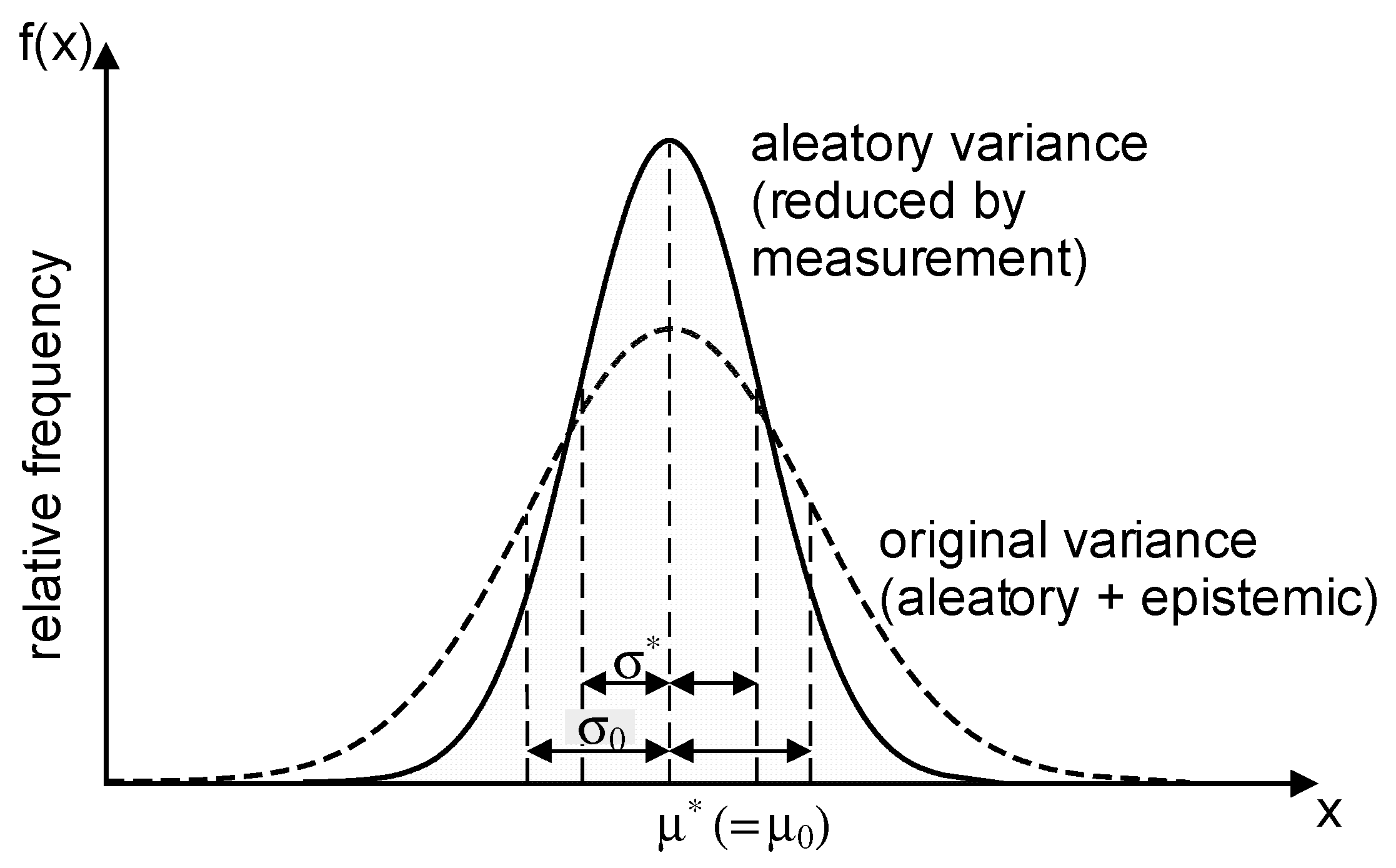
By means of sensitivity indices, the influence of a single parameter on the entire model can be analyzed based on its variance. Hora and Iman [34] introduced the conditional variance of a model, when one of its parameters is fixed to a deterministic value. In fact, the individual variances in stochastic analyses usually contain aleatory (random, nonreducible) and epistemic (reducible, inaccurate knowledge) parts. For structural systems only epistemic variances can be reduced (Figure 1). To determine the benefits of increased knowledge by monitoring or other measurements to reduce the variance, modified sensitivity indices should consider individual variance reductions, not the variance itself.
3.1. Proposed Method Based on SOBOL’ Indices
The proposed method decomposes the variance of a general model Y—no matter if analytical or numerical. While the initial model with originally large variances of all variables is termed Y0 (cf. Equation (1)), the best model with utmost reduced variances is denoted Y*. It comprises q parameters Xi*, each having a reduced variance V* (represented by a reduced standard deviation σ* in Figure 1).
Both models can be reformulated mathematically by means of variance decomposition (ANOVA HDMR), as shown before.
Thus, the variance V(Y0) of the initial model Y0 consists of q first-order variances Vi,0 and (q over 2) covariance terms Vi,j,0 (cf. Equation (6)). Y* is treated equivalently. Thus, the difference of the two decomposed variances in Equations (15) and (16) captures the extent of potential variance reduction ΔV*.
Employing Equations (15) and (16), this reduced variance can be decomposed, too. This decomposition is just analogous to that one in Section 2.2.
Herein, the reduced variance Vi* of a single parameter is interpreted as its individual improvement and it reads:
Thus, the potential variance reduction ΔV* from Equation (16) is given by:
If at first only a single parameter Xi* out of the q variables is improved, the model can be written as a function of q-1 “original” parameters Xj≠i,0 and one “improved” parameter Xi*.
Denoting the variance of this partly improved model V(Y(Xj≠i,0, Xi*)), the variance reduction by an improved knowledge about one parameter’s variance follows:
Now, considering two “improved” parameters Xi* and Xj*, the variance reduction of the entire model follows:
In the same way, one can increase the number of parameters with reduced variance gradually until finally all parameters Xj* except one single variable Xi,0 exhibit a reduced variance. This leads to:
Hence, the total variance reduction of such a model reads:
Finally, modified first-order sensitivity indices Si* are obtained from the ratio of single variance reductions ΔVi* (Equation (20)) to the total one ΔV* (acc. to Equation (18)). These indices capture the benefit of improving the knowledge about a single parameter Xi but neglecting any interactions with other reduced variances.
To evaluate the benefit of simultaneous measurements and belonging variance reductions of two or more parameters, higher-order modified sensitivity indices are conceivable, too.
However, each index Sj≠i * would require n additional model evaluations. In addition, relevant parameter combinations would have to be estimated in advance. Thus, such indices are omitted in the following evaluations.
3.2. Computational Implementation
A computational procedure to evaluate models is developed next. In general, it is based on the previously described computation of the original sensitivity indices in Section 2.2. An estimation of the modified sensitivity indices by correlation properties is no longer possible since the influence of reduced variances and the importance of a parameter would be mixed. A correlation coefficient analogue to the one in Equation (12) would still identify an important parameter even if its variance cannot be reduced. This is contrary to the basic idea of the modified sensitivity indices.
First, two sample matrices A* and B are determined analogously to the procedure in Section 2.2. Since the indices are no longer determined with correlation coefficients approach, it does not matter, whether they are stochastically independent or not. However, the pre-defined correlation within the matrices (usually the parameters are supposed to be independent) still needs to be maintained. Now, A* contains the realizations of reduced variance; B contains the realizations with the highest (initial) scatter. As before, both result vectors a* and b are evaluated by employing the model.
Next, further q matrices Ci* are generated. These matrices are assembled mainly from realizations of matrix B. Only column i comes from matrix A*. For each ci* the model needs to be evaluated again n times.
Finally, the computation of the modified sensitivity index follows analogue to Equation (24).
4. Application Case: A Model for Fatigue Lifetime Prediction of Pre-Stressed Concrete Bridges
The variance-based sensitivity indices were modified to analyze a complex stochastic model, which was set up to predict the residual fatigue lifetime of aged pre-stressed concrete bridges. As a reference serves a 50-year-old bridge in Germany [42]. Since the model includes, among other things, a finite element computation of the structural response and accumulation of damage over time, it is numerical and nondifferentiable. It involves interactions and uncertainties induced by the variance of the parameters. These different individual variances can be reduced, e.g., by on-site measurements, but, depending on the measurement methods and the individual aleatoric uncertainty, not to the same extent.
4.1. Reference Structure and Measurements
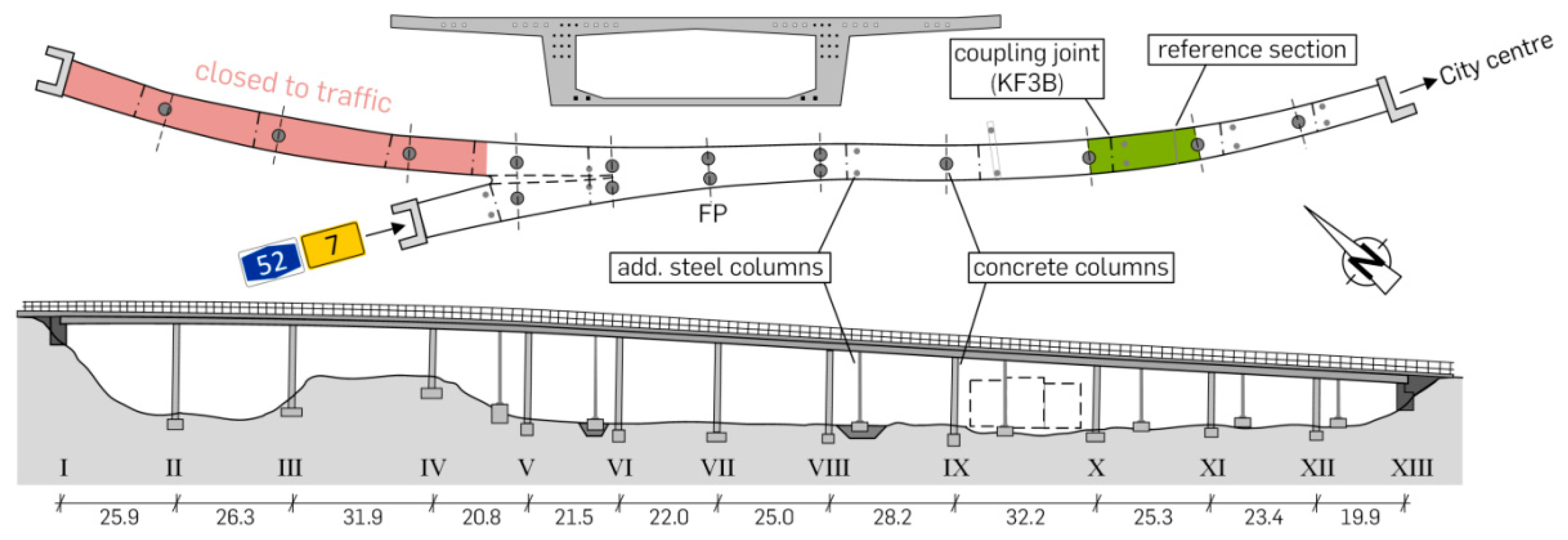
The reference structure for fatigue damage prediction is a 303 m long pre-stressed concrete bridge located in Düsseldorf, Germany (Figure 2). Since 1959, the box-girder-bridge has connected Düsseldorf’s city center to the German highway system. As it was a usual construction technique of that time, coupling joints connected consecutive construction parts and were located in each span at about one-fifth of the span length. The post-tensioned tendons had in general a parabolic profile, only few tendons ran straight along the upper and lower edges. Shortly after construction, first cracks were detected at the coupling joints. Because of the cracks and because it is a well-known weak point of aged bridges, fatigue of the tendons at the coupling joints was focused on during measurements and analyses.
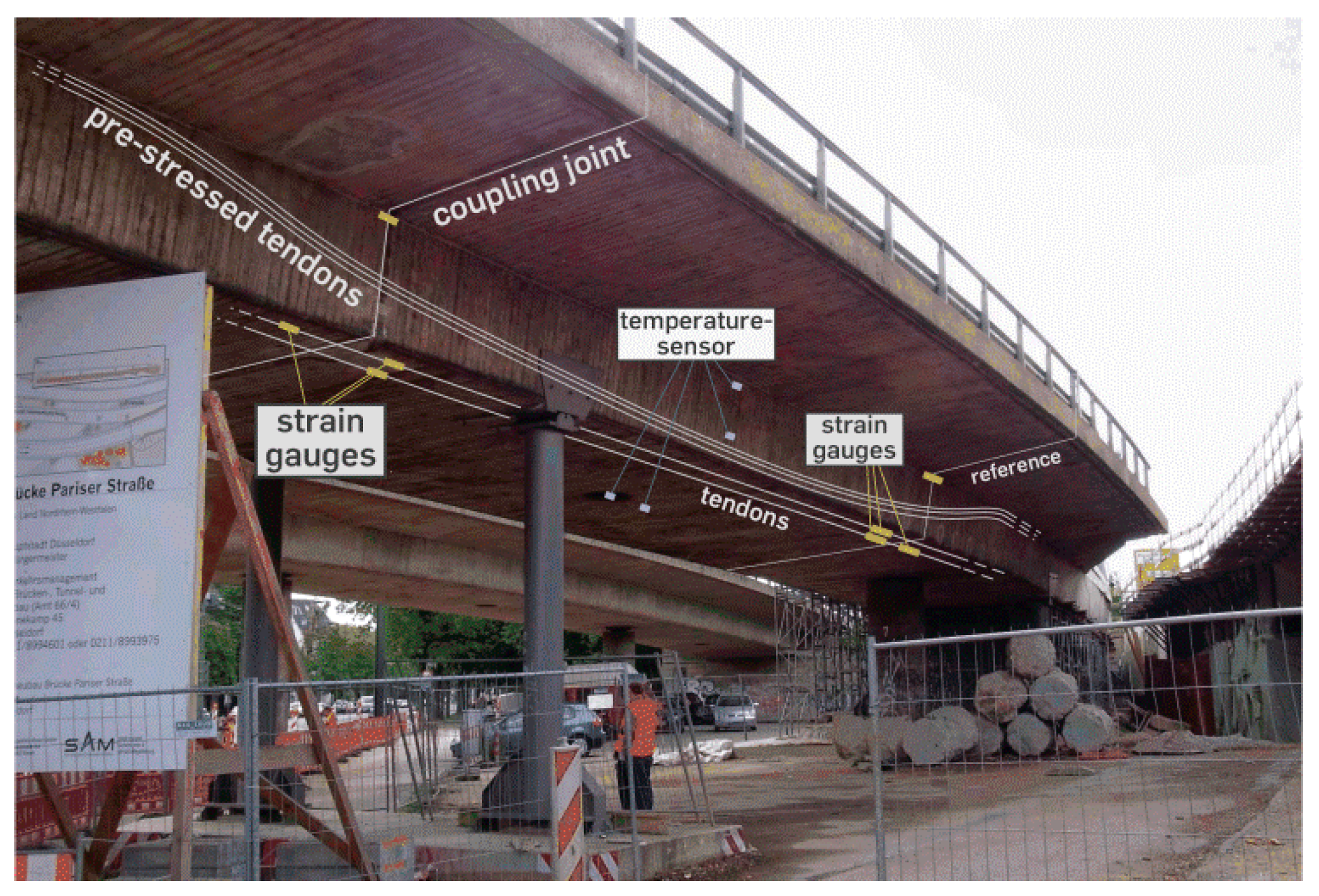
On-site, different measurements were carried out on the structure. In view of its certain deconstruction and replacement, both destructive and nondestructive tests could be performed. To serve as a reference, many different measurements were carried out to cover a wide range of potential impacts increasing the accuracy. Here, the geometry was determined by length measurements on-site while the strength of concrete and of the pre-stressing steel were evaluated on concrete cores and steel samples in the lab. Additionally, a strain monitoring of the pre-stressing steel and the temperature distribution (see Figure 3) was performed for several weeks.
4.2. Fatigue Lifetime Prediction Model for Pre-Stressed Concrete Bridges
An accurate prediction of the residual lifetime of pre-stressed concrete bridges, which are prone to fatigue, is hardly possible [43,44]. The special characteristic of high-cycle fatigue is sudden failure after many thousands or even millions of load cycles. For that, the fatigue damage progress is usually determined by extrapolating the frequency of calculated stress ranges from changing loads based on load models from the codes (e.g., [45]). Typical sources of uncertainty in the lifetime prediction for pre-stressed concrete road-bridges are:
- estimation and prognosis of loads (traffic loads and frequencies, temperature loads);
- calculation of stresses, including the nonlinearity after cracking (typically affected by the structural FE-model, cross-sectional and geometric parameters, material parameters, and stiffness);
- fatigue-related properties of the material resistance (represented by the S–N curve).
The model considered here is nonlinear, time-dependent, and able to predict the fatigue lifetime TFL of a pre-stressed concrete road-bridge, based on the accumulated fatigue damage D [46]. Fatigue failure occurs at damage D = 1 and is calculated by Miner’s rule [47,48]:
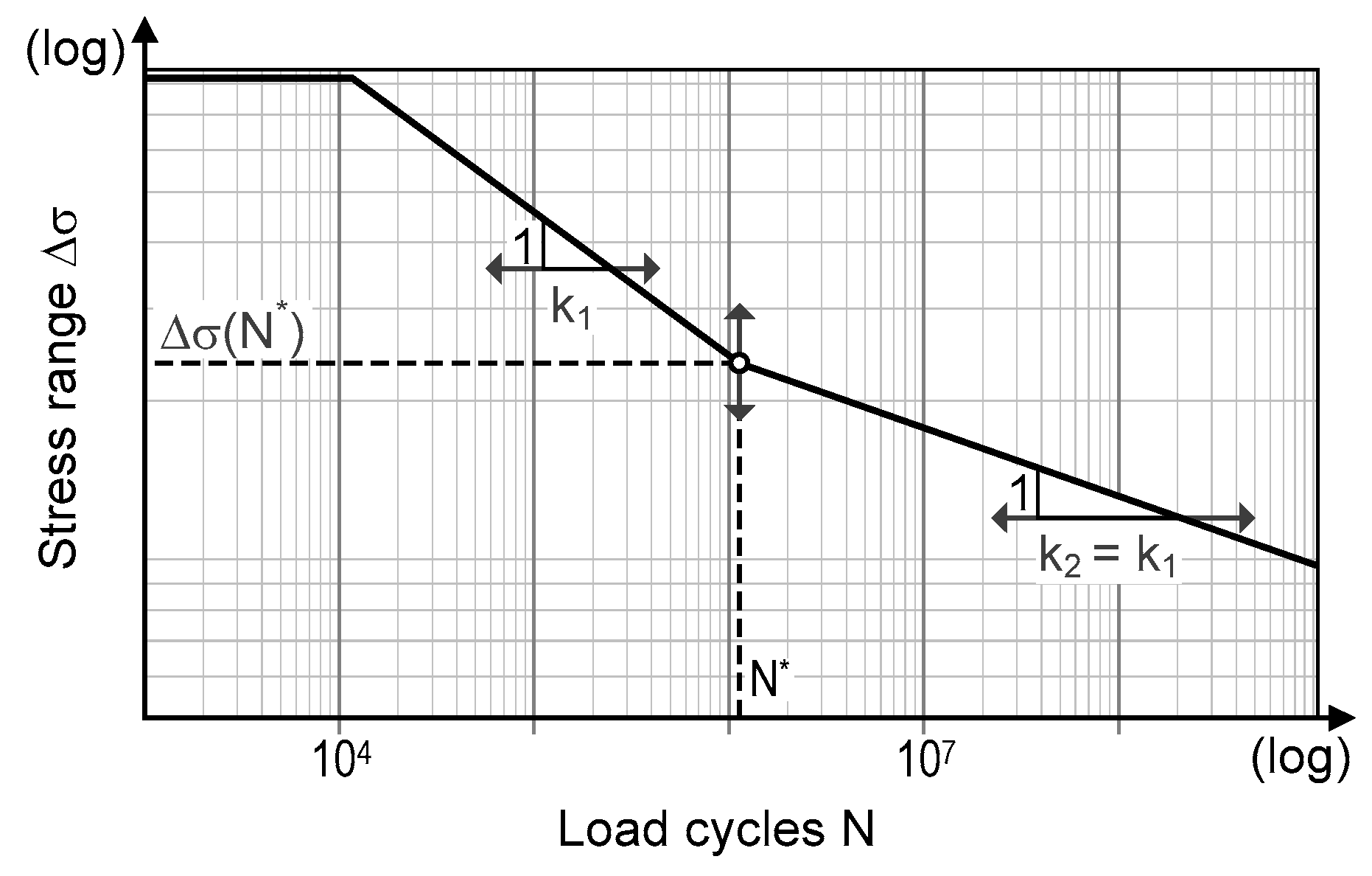
Load frequencies ni arise from traffic counts and prognosis and relative frequencies of individual vehicle types according to Eurocode 1–2 [45]. Load cycles until failure Ni are obtained from the S–N curve (Figure 4) according to the stress ranges Δσi. Stress ranges are determined at different load levels i by combining a structural model and an iterative computation method of stresses. For convenience, the internal forces have been determined on a linear-elastic FE beam model (Figure 5) separated from the computation of stresses on cross-sectional level to reduce the computational costs. An advantage of this approach is that superposition of the internal forces can still be applied for all load cases and evaluations of the complex FE-model can be reduced. Then the stresses are computed, employing an iterative procedure by Krüger and Mertzsch [49] to get accurate stresses in cracked concrete conditions. To also cover non-cracked (linear elastic) conditions, the original approach was slightly modified and now permits the neutral strain fiber to lie outside the cross-section (0 < ξ ≤ 2, with ξ = x/d and x being the height of compression zone and d the effective height), too.
That way, all stress ranges that are relevant for fatigue are treatable uniquely. In advance, the approach was checked to be sufficiently accurate and significantly reduces the computational effort for repeated simulation runs in comparison to a more detailed fatigue lifetime prognosis as presented elsewhere [50].
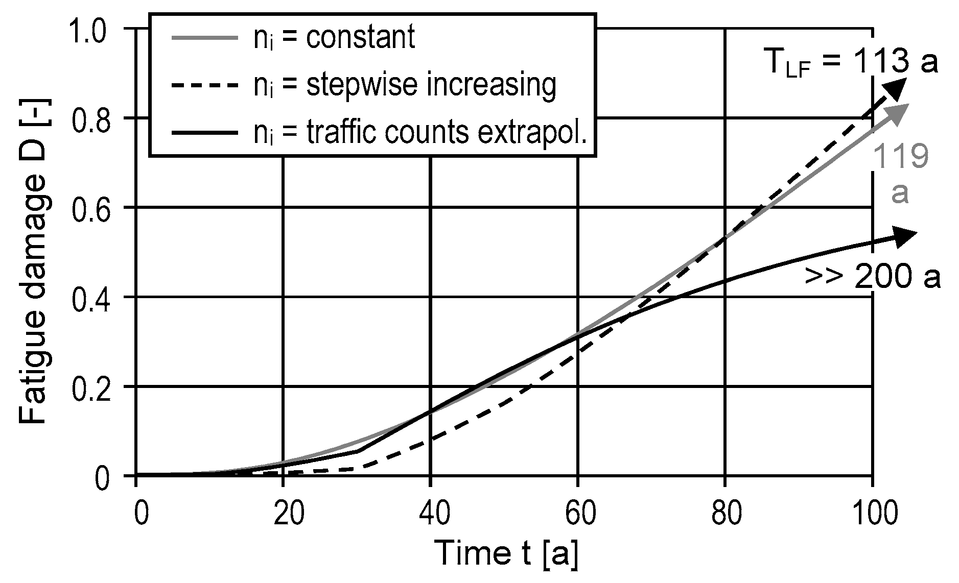
The evolution of fatigue damage is a nonlinear time-dependent process (exemplified in Figure 6), which is influenced, i.a., by creep and shrinkage and a global increase of traffic loads and frequencies (cf. Figure 6 and [43]). Hence, fatigue lifetime is usually determined by damage accumulation until failure occurs (Equation (30)). The simulations here aim to determine the total fatigue damage accumulated in 250 years D(t = 250 a). In total, five time intervals (Δt = 50 a), are assumed to cover the prediction period. Obviously, this is a quite rough discretization of time—especially for the first years, where the gradients are usually steep—but it was necessary to reduce the computational costs.
Creep, shrinkage and relaxation reduce the pre-strain in the tendons as a function of time. To cover creep and shrinkage, Bažant and Baweja’s model B3 [51] has been incorporated and simplified to a scaling function aCS(t) of the reduced pre-stress (details in [46]). Furthermore, hardening of concrete (compressive strength fc(t) and Young’s modulus Ec) is considered by a root function according to Eurocode 2 [52].
For traffic loads, the detailed fatigue load model FLM 4 from Eurocode 1–2 [45] was applied. It consists of five standardized truck types that are representative for heavyweight traffic in Europe. For convenience and to reduce the computational costs, the evaluations are restricted on truck type 3 of FLM 4 since it causes the highest stress ranges on the reference structure [50]. Mathematically, this simplification is conservative and delivers a lower bound of predicted lifetimes. Next, traffic- and temperature-induced stresses are superposed, while the latter ones have been computed from a histogram of discrete frequencies of linear vertical temperature gradients ΔT with time [53].
All the effects described before are considered in the model by 16 parameters:
- the width of the deck-slab bf, which represents the variability of the entire geometry;
- the effective height dp1 of the pre-stressed cross-section concerning tendon layer no. 1;
- a scaling factor for pre-stress losses by creep and shrinkage aCS;
- five (relevant) linear temperature gradients ΔTi;
- a scaling factor w3 for the traffic loads from FLM 4, truck no. 3;
- the cross-sectional area of a tendon Ap1;
- Young’s moduli of concrete Ec and pre-stressing steel Ep;
- two parameters to describe the S–N curve: its knee point Δσ(N*) at 106 load cycles and the slope of the high-cycle fatigue range (k2); for simplification k1 is set equal to k2.
These parameters are all subjected to uncertainty (cf. Table 1). Following a probabilistic approach, their scatter can be captured by normal and log-normal probability density functions (PDF). Table 1 also provides individual means and variances.
In addition to the original distribution parameters (μi,0, CVi,0), the reduced variances (as improved variation coefficient CV* with aleatory uncertainty only) are summarized in Table 1. The ratios of improved to original variances V*/V0 = σ*²/σ0² are a measure to assess the improvement of a single parameter. For values close to zero the improvement is significant, for Vi*/Vi,0 = 1 there is no reduction of the variance (by measurements). The given values are assumptions based on measurement data from the reference structure and information from the literature.
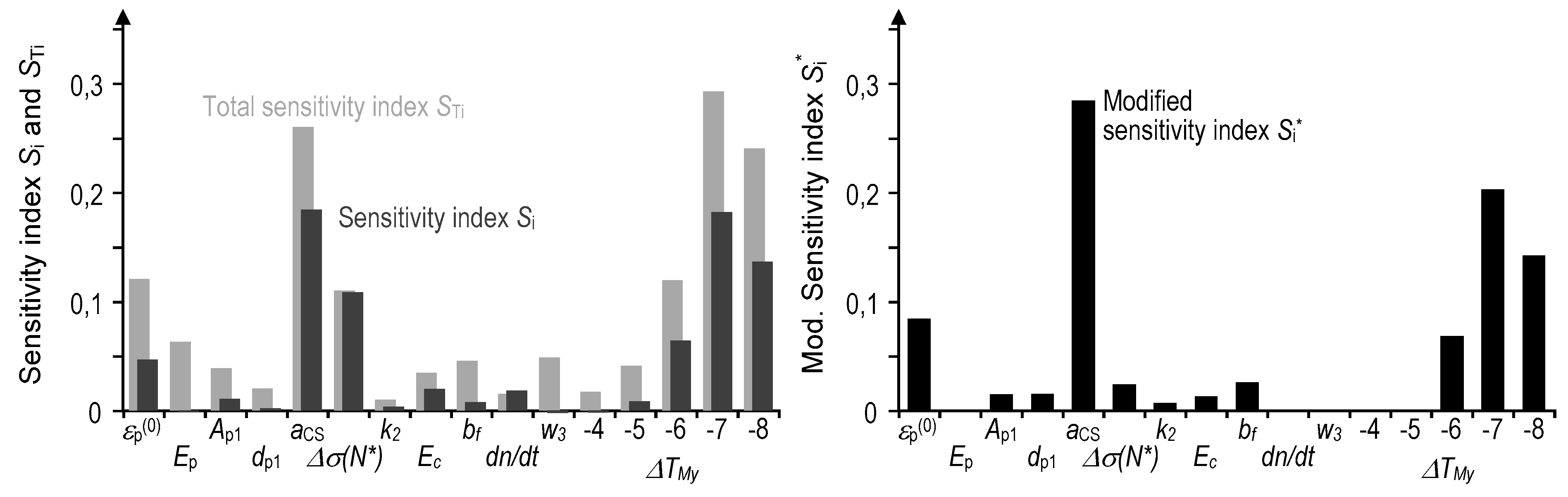
Original variance-based sensitivity indices Si and STi according to Section 2.1 (Figure 7, left) and reduced variances (as improved standard deviations σ* and as ratios of improved to original variances V*/V0) are given as well in Table 1. Before the sensitivity indices are determined, the result is logarithmically transformed (yi = log(xi)) to be more robust. Consequently, the data appears Gaussian distributed.
4.3. Stochastic Lifetime Prediction, Sensitivity Analysis and Evaluation of Modified Sensitivity Indices
The results of stochastic predictions of fatigue lifetime by Monte Carlo simulation are given in Table 2. They document a prognosis result when scatter of one single parameter is reduced by monitoring. More precisely, the table contains 16 sets of lognormal distribution characteristics LN(λ,ζ), means λ and standard deviations ζ, of accumulated damage D after 250 years. The shape of the distributions is assumed to be lognormal based on test statistics according to Kolmogorov–Smirnov (level of significance α = 0.05). Each set is determined based on n = 100 simulations for each parameter (n (2 + q) = 1800).
For comparison the characteristics for the initial model b (no improved variances) and the “best” model a* (all variances improved) are listed in the lower rows, too. Additionally, two columns of the prognosis result’s fractiles D0,90 and D0,99 have been computed as characteristic values. For the fatigue damage, the upper bound of the distribution is of interest and focused. Additionally, in comparison to the improvement from the initial model (b) to the best model (a*) the individual gains are quantified by relative specific improvements in the 6th and 7th column. The modified variance-based sensitivity indices are determined according to Equation (29) and are given in Table 2. They are also shown in Figure 7, right.
Next, original (Si and STi) and modified sensitivity indices (Si*) are opposed in Figure 7. For the presented fatigue lifetime model, at least six different variables show a significant impact (Si and STi) on the variance of the model. As a result of non-uniformly improved variances the results of the modified sensitivity indices (Si*) are individually shifted in comparison to the original sensitivity indices Si and STi in Table 2. Obviously, only relevant parameters characterized by a high sensitivity index STi and a seriously reduced variance (σi,0 >> σi*) lead to a significant variance reduction of the model. In contrast, a parameter without any variance reduction (σi,0 = σi*), like the scaling factor of traffic loads w3, does not change the model’s variance.
In total, three variables possess the highest original sensitivity indices: two temperature gradients ΔT(−7K), ΔT(−8K) and the scaling factor for creep and shrinkage aCS. Since the variance of aCS can be reduced at most (cf. Table 1) it also delivers the highest modified sensitivity index Si* (Figure 7, right)—as expected. The knee point of the S–N curve Δσ(N*) is a moderately important variable (Si ≈ STi ≈ 0.11), but its variance can hardly be reduced by measurements. Thus, it exhibits a low modified sensitivity index Si* = 0.03.
The impact of individual improvements is illustrated by four probability density functions (PDF) in Figure 8. Referenced is the original model Y0 with the highest variance—given by the computational result in b and marked by a dashed black line. This distribution function represents the initial prediction of the fatigue lifetime, having little knowledge about the parameters. Its total scatter comprises both, aleatory (random) and epistemic (lack of knowledge) parts. The “best” prediction model Y* using the computational result in a* yields another pdf marked as a solid black line in Figure 8. It visualizes the response when all variances are reduced to the greatest extent. Then the scatter is caused by aleatory parts uniquely. Compared to Y0 the variance of Y* is significantly lower while the mean is shifted, too.
Other cases when only one parameter’s variance is reduced by monitoring lie between these limit curves. The same holds true for the cumulative density functions (CDF) shown on the right in Figure 8. That way, the impact of individual measurements can be evaluated. Parameters that provide the closest shift to the “best” model yield the greatest benefit, if monitored. In this example, the scaling factor for creep and shrinkage aCS and the linear temperature gradient ΔT(−7 K) are the most important. They shift both distributions (CDF and PDF) significantly towards the best model’s one. However, an irrelevant parameter would yield curves similar to the initial one.
4.4. Convergence
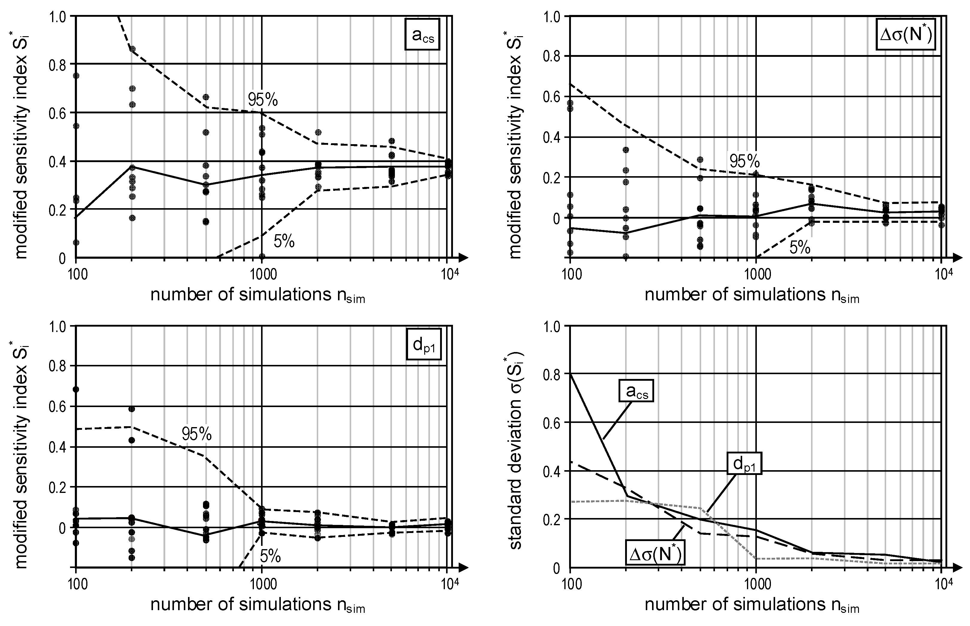
For reliable results, many thousand simulation runs are required as can be read from Figure 9 showing the convergence of the fatigue lifetime model. For the convergence plot the number of simulations n was increased incrementally from n = 100 to 104. For each n, the modified sensitivity indices were determined ten times with different sampling sets to assess their variation around the mean xm by means of the 5% and 95% fractiles (xm ± 1.645∙σ, assuming a Gaussian distribution) as a measure of variance. The results of the modified sensitivity indices for some of the 16 parameters are drawn in Figure 9. The selection comprises three types of parameters:
- The scaling factor of the pre-stress loss aCS in Figure 9 top left is a relevant parameter (STi-value is high) and can be reduced significantly (Vi*/Vi,0 << 1). Therefore, its modified sensitivity index Si* is expected to be high.
- The knee point of the S–N curve Δσ(N*) in Figure 9 top right is a relevant parameter (high STi-value) without significant variance reduction (Vi*/Vi,0 ≈ 1); thus, Si* is expected to be low.
- Third, the effective depth of the pre-stressing steel (dp1) on the lower left of Figure 9 has a low (original) total sensitivity index STi and even in case of a significant reduction of its variance, the modified sensitivity index can be expected to be low.
All three clearly converge for 104 simulations. At least 5000 simulation runs are recommended in this case. For smaller sample sizes, all modified sensitivity indices possess large variance. For less than 1000 simulations, the results should not be used at all. Then, some results with too-small sample sizes take on values even outside the reasonable range 0 ≤ Si* ≤ 1. As it could be expected, this is more likely for Si*-values close to zero. On the lower right, Figure 9 illustrates the convergence by means of the standard deviation. All three parameters converge similarly. Differences are seen purely caused by chance.
5. Conclusions
An extension to the established method of variance-based sensitivity indices originally proposed by Sobol’ is developed. The modified sensitivity indices are suited to quantify potential benefits of measurements and monitoring measures in advance. The enhanced indices are mathematically derived, and its numerical implementation based on stochastic simulation is exemplified on a model for fatigue lifetime prediction of a reference structure.
For the 50-year-old pre-stressed concrete bridge in Germany, the indices indicate that the measurement of residual pre-stress in the tendons after creep and shrinkage and the measurement of temperature loads are most meaningful. It can be found that the best parameters to be measured (high Si*) are those impairing a model’s variance significantly (characterized by high-variance-based indices Si and STi) and simultaneously having a great potential for variance reduction by monitoring. In comparison to others, they possess the highest modified sensitivity indices.
To support experts’ sound decisions on qualified measures to take the complex interaction of variance reduction and its influence on a model can be assessed in advance and quantified with reasonable effort by the newly proposed modified sensitivity indices Si*. In view of an ever-increasing stock of aged infrastructure buildings worldwide, the modified indices might help to save money and resources, avoiding unnecessary measurements in the future.
Author Contributions
Conceptualization, D.S., M.A.A. and P.M.; methodology, D.S.; software, D.S.; investigation, D.S.; data curation, D.S.; validation, D.S. and M.A.A.; writing—original draft preparation, D.S.; writing—review and editing, M.A.A. and P.M.; visualization, D.S.; supervision, M.A.A. and P.M.; project administration, M.A.A.; funding acquisition, M.A.A. and P.M. All authors have read and agreed to the published version of the manuscript.
Funding
This research was funded by the German Research Foundation (Deutsche Forschungsgemeinschaft DFG), grant number 221282822.
Institutional Review Board Statement
Not applicable.
Informed Consent Statement
Not applicable.
Data Availability Statement
The datasets generated during the study are available from the corresponding author on reasonable request.
Conflicts of Interest
The authors declare no conflict of interest.
References
- Ahrens, M.A.; Mark, P. Lebensdauersimulation von Betontragwerken. Beton- und Stahlbetonbau. 2011, 106, 220–230. [Google Scholar] [CrossRef]
- Sanio, D.; Ahrens, M.A. Identification of relevant but stochastic input parameters for fatigue assessment of pre-stressed concrete bridges by monitoring. In Proceedings of the 1st International Conference on Uncertainty Quantification in Computational Sciences and Engineering (UNCECOMP 2015), Crete Island, Greece, 25–27 May 2015; Papadrakakis, M., Papadopoulos, V., Stefanou, G., Eds.; pp. 947–960. [Google Scholar]
- Ambrozinski, L.; Packo, P.; Pieczonka, L.; Stepinski, T.; Uhl, T.; Staszewski, W.J. Identification of material properties—efficient modelling approach based on guided wave propagation and spatial multiple signal classification. Struct. Control. Health Monit. 2015, 22, 969–983. [Google Scholar] [CrossRef]
- Žnidarič, A.; Kreslin, M.; Lavrič, I.; Kalin, J. Simplified Approach to Modelling Traffic Loads on Bridges. Procedia Soc. Behav. Sci. 2012, 48, 2887–2896. [Google Scholar] [CrossRef] [Green Version]
- Löschmann, J.; Ahrens, A.; Dankmeyer, U.; Ziem, E.; Mark, P. Methoden zur Reduktion des Teilsicherheitsbeiwerts für Eigenlasten bei Bestandsbrücken. Beton. Und. Stahlbetonbau. 2017, 112, 506–516. [Google Scholar] [CrossRef]
- Ahrens, M.A. Precision-assessment of lifetime prognoses based on SN-approaches of RC-structures exposed to fatigue loads. In Life-Cycle and Sustainability of Civil Infrastructure Systems. In Proceedings of the 3rd International Symposium on Life-Cycle Civil Engineering (IALCCE), IALCCE 12, Vienna, Austria, 3–6 October 2012; Strauss, A., Frangopol, D., Berg-Meister, K., Eds.; CRC Press: Hoboken, NJ, USA, 2012; p. 109, ISBN 9780203103364. [Google Scholar]
- Gao, R.; Li, J.; Ang, A.H.-S. Stochastic analysis of fatigue of concrete bridges. Struct. Infrastruct. Eng. 2019, 15, 925–939. [Google Scholar] [CrossRef]
- Walpole, R.E.; Myers, R.H.; Myers, S.L.; Ye, K. Probability & Statistics for Engineers & Scientists, 9. Auflage; Prentice Hall: Boston, MS, USA, 2012; ISBN 0321629116. [Google Scholar]
- Strauss, A.; Hoffmann, S.; Wan-Wendner, R.; Bergmeister, K. Structural assessment and reliability analysis for existing engineering structures, applications for real structures. Struct. Infrastruct. Eng. 2009, 5, 277–286. [Google Scholar] [CrossRef]
- Saltelli, A.; Ratto, M.; Andres, T.; Campolongo, F.; Cariboni, J.; Gatelli, D.; Saisana, M.; Tarantola, S. Global Sensitivity Analysis: The Primer; John Wiley & Sons: Chichester, UK, 2008; ISBN 0470725176. [Google Scholar]
- Iooss, B.; Lemaître, P. A review on global sensitivity analysis methods // A Review on Global Sensitivity Analysis Methods. In Uncertainty Management in Simulation-Optimization of Complex Systems: Algorithms and Applications, Dellino, G., Meloni, C., Eds.; Springer: Boston, MS, USA, 2015; pp. 101–122. ISBN 978-1-4899-7546-1. [Google Scholar]
- Augusti, G.; Baratta, A.; Casciati, F. Probabilistic Methods in Structural Engineering; Chapman and Hall/CRC: Boca Raton, FL, USA, 2014; ISBN 9781482267457. [Google Scholar]
- Saltelli, A.; Annoni, P.; Azzini, I.; Campolongo, F.; Ratto, M.; Tarantola, S. Variance based sensitivity analysis of model output. Design and estimator for the total sensitivity index. Comput. Phys. Commun. 2010, 181, 259–270. [Google Scholar] [CrossRef]
- Wainwright, H.M.; Finsterle, S.; Jung, Y.; Zhou, Q.; Birkholzer, J.T. Making sense of global sensitivity analyses. Comput. Geosci. 2014, 65, 84–94. [Google Scholar] [CrossRef]
- Sanio, D.; Obel, M.; Mark, P. Screening methods to reduce complex models of existing structures. In Proceedings of the 17th International Probabilistic Workshop (IPW), Edinburgh, UK, 11–13 September 2019; pp. 51–56. [Google Scholar]
- Campolongo, F.; Cariboni, J.; Saltelli, A. An effective screening design for sensitivity analysis of large models. Environ. Model. Softw. 2007, 22, 1509–1518. [Google Scholar] [CrossRef]
- Morris, M.D. Factorial Sampling Plans for Preliminary Computational Experiments. Technometrics 1991, 33, 161. [Google Scholar] [CrossRef]
- Sobol, I.M. Global sensitivity indices for nonlinear mathematical models and their Monte Carlo estimates. Math. Comput. Simul. 2001, 55, 271–280. [Google Scholar] [CrossRef]
- Campolongo, F.; Tarantola, S.; Saltelli, A. Tackling quantitatively large dimensionality problems. Comput. Phys. Commun. 1999, 117, 75–85. [Google Scholar] [CrossRef]
- Bien, J.; Kużawa, M.; Kamiński, T. Strategies and tools for the monitoring of concrete bridges. Struct. Concr. 2020, 21, 1227–1239. [Google Scholar] [CrossRef]
- Brühwiler, E. Fatigue safety examination of riveted railway bridges using monitored data. In Bridge Maintenance, Safety, Management and Life Extension, Proceedings of the 7th International Conference of Bridge Maintenance, Safety and Management. IABMAS 2014, Shanghai, China, 7–11 July 2014; Chen, A., Frangopol, D.M., Eds.; CRC Press: Boca Raton, FL, USA, 2014; pp. 1169–1176. ISBN 9781138001039. [Google Scholar]
- Frangopol, D.M.; Strauss, A.; Kim, S. Bridge Reliability Assessment Based on Monitoring. J. Bridg. Eng. 2008, 13, 258–270. [Google Scholar] [CrossRef]
- Bayane, I.; Mankar, A.; Brühwiler, E.; Sørensen, J.D. Quantification of traffic and temperature effects on the fatigue safety of a reinforced-concrete bridge deck based on monitoring data. Eng. Struct. 2019, 196, 109357. [Google Scholar] [CrossRef]
- Treacy, M.A.; Brühwiler, E. Action effects in post-tensioned concrete box-girder bridges obtained from high-frequency monitoring. J. Civ. Struct. Health Monit. 2014, 5, 11–28. [Google Scholar] [CrossRef]
- Nair, A.; Cai, C.S. Acoustic emission monitoring of bridges: Review and case studies. Eng. Struct. 2010, 32, 1704–1714. [Google Scholar] [CrossRef]
- Marx, S.; von der Haar, C.; Liebig, J.P.; Grünberg, I.J. Bestimmung der Verkehrseinwirkung auf Brückentragwerke aus Messungen an Fahrbahnübergangskonstruktionen. Bautech 2013, 90, 466–474. [Google Scholar] [CrossRef]
- Uva, G.; Porco, F.; Fiore, A.; Mezzina, M. Proposal of a methodology for assessing the reliability of in situ concrete tests and improving the estimate of the compressive strength. Constr. Build. Mater. 2013, 38, 72–83. [Google Scholar] [CrossRef]
- Malhotra, V.M. In Situ/Nondestructive Testing of Concrete; American Concrete Institute (ACI): Detroid, MI, USA, 1984. [Google Scholar]
- Der Kiureghian, A.; Ditlevsen, O. Aleatory or epistemic? Does it matter? Struct. Saf. 2009, 31, 105–112. [Google Scholar] [CrossRef]
- Zhou, L.; Yan, G.; Wang, L.; Ou, J. Review of Benchmark Studies and Guidelines for Structural Health Monitoring. Adv. Struct. Eng. 2013, 16, 1187–1206. [Google Scholar] [CrossRef]
- ACI Committee 444. PRC-444.2-21: Structural Health Monitoring Technologies for Concrete Structures. Report; ACI Reports ACI PRC-444.2-21, Farmington Hills, Mich. 2021. Available online: https://www.concrete.org/store/productdetail.aspx?ItemID=444221 (accessed on 18 August 2021).
- Pozo, F.; Tibaduiza, D.; Vidal, Y. Sensors for Structural Health Monitoring and Condition Monitoring. Sensors 2021, 21, 1558. [Google Scholar] [CrossRef]
- Tarantola, S.; Gatelli, D.; Mara, T. Random balance designs for the estimation of first order global sensitivity indices. Reliab. Eng. Syst. Saf. 2006, 91, 717–727. [Google Scholar] [CrossRef] [Green Version]
- Hora, S.C.; Iman, R.L. Comparison of Maximus/Bounding and Bayes/Monte Carlo for Fault Tree Uncertainty Analysis. 1986. Available online: https://www.osti.gov/biblio/5824798 (accessed on 22 October 2021).
- Cukier, R.I.; Levine, H.B.; Shuler, K.E. Nonlinear sensitivity analysis of multiparameter model systems. J. Comput. Phys. 1978, 26, 1–42. [Google Scholar] [CrossRef]
- Sobol’, I. Theorems and examples on high dimensional model representation. Reliab. Eng. Syst. Saf. 2003, 79, 187–193. [Google Scholar] [CrossRef]
- Archer, G.E.B.; Saltelli, A.; Sobol, I.M. Sensitivity measures, anova-like Techniques and the use of bootstrap. J. Stat. Comput. Simul. 1997, 58, 99–120. [Google Scholar] [CrossRef]
- Ökten, G.; Liu, Y. Randomized quasi-Monte Carlo methods in global sensitivity analysis. Reliab. Eng. Syst. Saf. 2021, 210, 107520. [Google Scholar] [CrossRef]
- Glen, G.; Isaacs, K. Estimating Sobol sensitivity indices using correlations. Environ. Model. Softw. 2012, 37, 157–166. [Google Scholar] [CrossRef]
- Saltelli, A.; Tarantola, S.; Chan, K.P.-S. A Quantitative Model-Independent Method for Global Sensitivity Analysis of Model Output. Technometrics 1999, 41, 39–56. [Google Scholar] [CrossRef]
- Piano, S.L.; Ferretti, F.; Puy, A.; Albrecht, D.; Saltelli, A. Variance-based sensitivity analysis: The quest for better estimators and designs between explorativity and economy. Reliab. Eng. Syst. Saf. 2021, 206, 107300. [Google Scholar] [CrossRef]
- Sanio, D.; Ahrens, M.A.; Mark, P.; Rode, S. Untersuchung einer 50 Jahre alten Spannbetonbrücke zur Genauigkeitssteigerung von Lebensdauerprognosen. Beton- und Stahlbetonbau. 2014, 109, 128–137. [Google Scholar] [CrossRef]
- Sanio, D.; Ahrens, M.; Mark, P. Detecting the limits of accuracy of lifetime predictions by structural monitoring. In Proceedings of the Bridge Maintenance, Safety, Management and Life Extension; Chen, A., Frangopol, D.M., Eds.; CRC Press: Boca Raton, FL, USA, 2014; pp. 416–423. [Google Scholar]
- Sanio, D.; Ahrens, M.A.; Mark, P. Tackling uncertainty in structural lifetime evaluations. Beton- und Stahlbetonbau. 2018, 113, 48–54. [Google Scholar] [CrossRef]
- EN 1991-2: Eurocode 1: Actions on Structures: Part 2: Traffic Loads on Bridges; CEN: Brussels, Belgium, 2010.
- Sanio, D. Accuracy of Monitoring-Based Lifetime-Predictions for Prestressed Concrete Bridges Prone to Fatigue. Ph.D. Thesis, Ruhr-Universität Bochum, Bochum, Germany, 2017. [Google Scholar]
- Pålmgren, A. Die Lebensdauer von Kugellagern. Z. Des Ver. Dtsch. Ing. 1924, 68, 339–341. [Google Scholar]
- Miner, M.A. Cumulative Damage in Fatigue. J. Appl. Mech. 1945, 12, A159–A164. [Google Scholar] [CrossRef]
- Krüger, W.; Mertzsch, O. Zum Trag- und Verformungsverhalten bewehrter Betonquerschnitte im Grenzzustand der Gebrauchstauglichkeit; DAfStb-Heft No. 533; Beuth: Berlin, Germany, 2006. [Google Scholar]
- Sanio, D.; Ahrens, M.A.; Mark, P. Lifetime predictions of pre-stressed concrete bridges—Evaluating parameters of relevance using Sobol’-indices. Civ. Eng. Des. 2021. [Google Scholar] [CrossRef]
- Bažant, Z.P.; Baweja, S. Creep and shrinkage prediction model for analysis and design of concrete structures—model B3. Mater. Struct. 1995, 28, 357–365. [Google Scholar] [CrossRef]
- EN 1992-2: Eurocode 2: Design of Concrete Structures: Part 2: Concrete Bridges—Design and Detailing Rules; CEN: Brussels, Belgium, 2010.
- Sanio, D.; Mark, P.; Ahrens, M.A. Temperaturfeldberechnung für Brücken. Beton- und Stahlbetonbau. 2017, 112, 85–95. [Google Scholar] [CrossRef]
Figure 1.
Probability density functions of a variable with original and reduced variance due to increased knowledge.
Figure 1.
Probability density functions of a variable with original and reduced variance due to increased knowledge.

Figure 2.
Reference structure Pariser Straße in Düsseldorf, Germany—side and top views along with a general cross-section.
Figure 2.
Reference structure Pariser Straße in Düsseldorf, Germany—side and top views along with a general cross-section.

Figure 3.
Strain and temperature monitoring of the reference structure.

Figure 4.
Typical S–N curve for high-strength steel and its variables indicated by arrows.

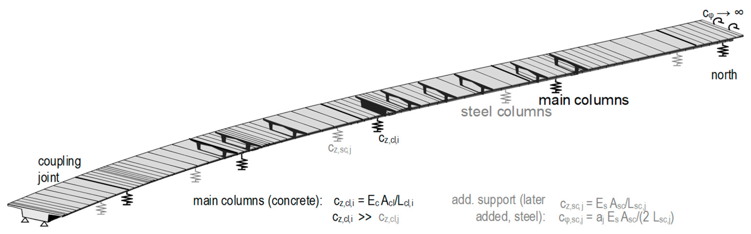
Figure 5.
Finite-element model of the reference structure; beam elements (cross-sections for visualization) and boundary conditions by springs and supports.
Figure 5.
Finite-element model of the reference structure; beam elements (cross-sections for visualization) and boundary conditions by springs and supports.

Figure 6.
Damage evolution from a deterministic model with time-dependent stress ranges and three different approaches of the load frequency.
Figure 6.
Damage evolution from a deterministic model with time-dependent stress ranges and three different approaches of the load frequency.

Figure 7.
Original and total (left) versus modified sensitivity indices (right) for the reference bridge.
Figure 7.
Original and total (left) versus modified sensitivity indices (right) for the reference bridge.

Figure 8.
Probability and cumulative density functions of the original (Y0) and the best model (Y*) along with two cases when only one parameter’s scatter is reduced by monitoring.
Figure 8.
Probability and cumulative density functions of the original (Y0) and the best model (Y*) along with two cases when only one parameter’s scatter is reduced by monitoring.

Figure 9.
Convergence of the modified sensitivity index for three parameters of the lifetime prediction model.
Figure 9.
Convergence of the modified sensitivity index for three parameters of the lifetime prediction model.


Table 1.
Stochastic variables with initial (original) distribution characteristics (μi,0, σi,0) and reduced variances (σi*), as well as Sobol’s sensitivity indices.
Table 1.
Stochastic variables with initial (original) distribution characteristics (μi,0, σi,0) and reduced variances (σi*), as well as Sobol’s sensitivity indices.
| Variable i | Distribution | Orig. Distribution | Improvement | Sensitivity Indices | |||||
|---|---|---|---|---|---|---|---|---|---|
| μi,0 | CVi,0 | CVi* | Vi*/Vi,0 | Si | STi | ||||
| Pre-strain | εp(0) | [‰] | N | 2.175 | 0.046 | 0.014 | 0.09 | 0.05 | 0.12 |
| Young’s modulus of steel | Ep | [N/mm2] | N | 205,000 | 0.030 | 0.024 | 0.63 | ~0 | 0.06 |
| Scaling factor for creep and shrinkage | aCS | [-] | N | 1 | 0.100 | 0.050 | 0.25 | 0.18 | 0.26 |
| Young’s modulus of concrete | Ec | [N/mm2] | LN | 33,000 | 0.091 | 0.045 | 0.25 | 0.02 | 0.04 |
| S–N curve: | LN | 120 | 0.008 | 0.063 | 0.88 | 0.11 | 0.11 | ||
| knee point | Δσ (N*) | [N/mm2] | |||||||
| slope | k2 | [-] | LN | 7 | 0.071 | 0.043 | 0.36 | 0.004 | 0.01 |
| Width of the deck-slab | bf | [m] | N | 4.95 | 0.101 | 0.001 | <0.01 | 0.01 | 0.05 |
| Area of a tendon | Ap1 | [cm2] | N | 26.55 | 0.016 | 0.007 | 0.21 | 0.01 | 0.04 |
| Effective height for tendon layer 1 | dp1 | [m] | N | 1.31 | 0.008 | 0.002 | 0.04 | 0.002 | 0.02 |
| Gradient of load cycles per year | dn/dt | N | 15,000 | 0.333 | 0.317 | 0.9 | 0.02 | 0.02 | |
| Scaling factor for FLM4-type 3 | w3 | [-] | N | 1 | 0.100 | 0.100 | 1 | ~0 | 0.05 |
| Temperature gradients (scaled): | 1 | 0.008 | 0.141 | 0.5 | ~0 | 0.02 | |||
| ΔT(−4 K) | N | ||||||||
| ΔT(−5 K) | N | 1 | 0.200 | 0.141 | 0.5 | 0.01 | 0.04 | ||
| ΔT(−6 K) | N | 1 | 0.200 | 0.141 | 0.5 | 0.06 | 0.18 | ||
| ΔT(−7 K) | N | 1 | 0.200 | 0.141 | 0.5 | 0.18 | 0.29 | ||
| ΔT(−8 K) | N | 1 | 0.200 | 0.141 | 0.5 | 0.14 | 0.24 | ||
Table 2.
Improved distribution parameters, specific improvements of the target variable and modified sensitivity indices.
Table 2.
Improved distribution parameters, specific improvements of the target variable and modified sensitivity indices.
| Variable i | Distribution Characteristics When i Is Improved | Relative Fractile Change | Mod. Sensitivity Index | ||||||
|---|---|---|---|---|---|---|---|---|---|
| λ | ζ | D0,90 | D0,99 | D0,90 | D0,99 | Si* | |||
| Pre-strain | εp(0) | [‰] | −1.94 | 3.189 | 8.535 | 238.8 | +11% | +16% | 0.09 |
| Young’s modulus of steel | Ep | [N/mm2] | −1.93 | 3.254 | 9.350 | 280.2 | +1% | +1% | 0.001 |
| Area of the tendon | Ap1 | [cm2] | −1.94 | 3.243 | 9.156 | 271.3 | +3% | +4% | 0.02 |
| Effective depth of the tendon | dp1 | [m] | −1.93 | 3.243 | 9.283 | 275.0 | +% | +3% | 0.02 |
| Scaling factor creep and shrinkage | aCS | [-] | −1.95 | 3.026 | 6.851 | 161.8 | +31 % | +45% | 0.29 |
| S–N curve: | |||||||||
| knee point | Δσ(N*) | [N/mm2] | −1.92 | 3.236 | 9.291 | 273.2 | +2% | +4% | 0.03 |
| slope | k2 | [-] | −1.93 | 3.249 | 9.324 | 278.0 | +1% | +2% | 0.01 |
| Young’s modulus of concrete | Ec | [N/mm2] | −1.97 | 3.245 | 8.893 | 263.9 | +7% | +7% | 0.01 |
| Width of the deck-slab | bf | [m] | −1.96 | 3.235 | 8.857 | 260.1 | +7% | +9% | 0.03 |
| Gradient of load cycles in time | dn/dt | −1.93 | 3.257 | 9.406 | 282.7 | +0% | +0% | ~0 | |
| Scaling factor FLM4-type 3 | w3 | [-] | −1.92 | 3.262 | 9.556 | 288.7 | −% | −2% | ~0 |
| Temperature gradient: | |||||||||
| ΔT(−4 K) | −1.96 | 3.284 | 9.469 | 292.8 | −0% | −4% | ~0 | ||
| ΔT(−5 K) | −1.98 | 3.260 | 9.004 | 271.4 | +5% | +4% | ~0 | ||
| ΔT(−6 K) | −2.08 | 3.201 | 7.519 | 213.2 | +23% | +26% | 0.07 | ||
| ΔT(−7 K) | −2.25 | 3.094 | 5.570 | 141.1 | +46% | +53% | 0.20 | ||
| ΔT(−8 K) | −2.19 | 3.143 | 6.268 | 167.1 | +38% | +43% | 0.14 | ||
| “best” model a* with V* | −2.92 | 2.349 | 1.099 | 12.8 | +100% | +100% | - | ||
| initial model b with V0 | −1.93 | 3.255 | 9.433 | 283.0 | ±0 | ±0 | - | ||
Publisher’s Note: MDPI stays neutral with regard to jurisdictional claims in published maps and institutional affiliations. |
© 2021 by the authors. Licensee MDPI, Basel, Switzerland. This article is an open access article distributed under the terms and conditions of the Creative Commons Attribution (CC BY) license (https://creativecommons.org/licenses/by/4.0/).
Share and Cite
MDPI and ACS Style
Sanio, D.; Ahrens, M.A.; Mark, P. Modification of Variance-Based Sensitivity Indices for Stochastic Evaluation of Monitoring Measures. Infrastructures 2021, 6, 149. https://0-doi-org.brum.beds.ac.uk/10.3390/infrastructures6110149
AMA Style
Sanio D, Ahrens MA, Mark P. Modification of Variance-Based Sensitivity Indices for Stochastic Evaluation of Monitoring Measures. Infrastructures. 2021; 6(11):149. https://0-doi-org.brum.beds.ac.uk/10.3390/infrastructures6110149
Chicago/Turabian StyleSanio, David, Mark Alexander Ahrens, and Peter Mark. 2021. "Modification of Variance-Based Sensitivity Indices for Stochastic Evaluation of Monitoring Measures" Infrastructures 6, no. 11: 149. https://0-doi-org.brum.beds.ac.uk/10.3390/infrastructures6110149