
Risk-Based Criticality Assessment for Smart Critical Infrastructures


1
Department of Information Systems, King Khalid University, Abha City 62529, Saudi Arabia
2
Department of Informatics and Networked Systems, University of Pittsburgh, Pittsburgh, PA 15213, USA
*
Author to whom correspondence should be addressed.
†
Current address: Guraiger Campus, Abha City 62529, Saudi Arabia.
Infrastructures 2022, 7(1), 3; https://0-doi-org.brum.beds.ac.uk/10.3390/infrastructures7010003
Submission received: 5 November 2021
/
Revised: 19 December 2021
/
Accepted: 21 December 2021
/
Published: 25 December 2021
(This article belongs to the Special Issue Smart Infrastructures Feature Papers)
Abstract
:Today, critical infrastructure is more interconnected, which allows more vulnerabilities in the case of disasters. In addition, the effect of one infrastructure can lead to one or more cascading failures in another infrastructure due to the dependency complexity between them. This article introduces a holistic approach using network indicators and machine learning to better understand the geographical representation of critical infrastructure. Previous work on a similar model was based on a single measure; such as in fashion, this paper introduces four measures utilized to identify the most vital geographic zone in the city. The model aims to increase resilience, focusing on the preparedness phase by assessing the essential nodes of infrastructure, which allows more space to adopt risk mitigation strategies before any disturbance event. Holding in-depth knowledge of the vital zones of small scales and accordingly ranking them will positively improve the overall system resilience.
1. Introduction
Today, our countries, national safety, financial success, and social health are primarily reliant on a collection of highly interdependent critical infrastructures. Numerous cases containing these systems can be viewed, including the power networks system, natural gas infrastructure, communication infrastructure, water systems, and transportation systems. Understanding these infrastructures’ behavior is crucial, particularly when stressed or under attack. Infrastructures attacks include a wide range of physical attacks and virtual attacks such as climate change and pandemics. One way to understand such behavior can be reflected by obtaining resilience. Resilience in this scenario can be defined as the ability of the system to prepare, absorb, and recover in a reasonable time. Metrics and models related to infrastructure resilience can exhibit signs that affect the interdependent critical infrastructures’ performances and operational features. These models and measures require introducing interdependencies between infrastructures to present detailed descriptions of infrastructure resilience such as [1,2].
Resilience has also been defined as the capacity of a system to absorb disturbance, undergo change, and preserve approximately the equivalent function, structure, identity, and feedback [3]. Resilient infrastructure is different from sustainable infrastructure, which refers to designing, building, and operating the infrastructure through the day-to-day function in ways that do not reduce the social, economic, and ecological operations demanded to maintain human equity, diversity, and the functionality of natural systems. Resilience encompasses three primary stages based on the functionality timeline: preparedness, recovery, and restoration. Preparedness is a significant phase in promoting the function of interdependent critical infrastructures, and for any infrastructure to be prepared, an enhanced risk mitigation mechanism should be employed to the critical elements of that system.
Nevertheless, determining the most critical components has been challenging, particularly in the state of multiple infrastructures. For example, based on the Department of Homeland Security’s last report [4], there are more than 16 infrastructures that are considered critical; yet, these infrastructures are not formed in an isolated form but more in an interconnected fashion, and this raises the complexity of precisely locating the most critical nodes.
This paper introduces a holistic approach that uses an indicator-based approach, a network-based approach, and machine learning to better understand the geographical representation of the critical infrastructures. Understanding such a model will allow for the accurate measurement of infrastructures elements and determining which part has the most impact and then will help avoid any future disaster by applying the protection mechanism on that element.
The remainder of the paper is designed as follows. Section 2 reviews related work on critical infrastructure analysis to identify the most exposed or significant elements. Section 3 presents our methodology to identify and assess a metropolitan city’s most vital geographic zones. Section 4 provides numerical results from a case study with our suggested approach, including a risk analysis. Lastly, Section 5 presents our conclusions.
2. Background and Related Work
One way of modeling infrastructure in literature has been conducted through the network modeling [5]. By modeling the infrastructure as a network, the implementation of centrality approaches to critical infrastructure protection and mitigation control can be applied. However, this approach has been applied to a single infrastructure, and there is no coherent framework apprehending other interdependent infrastructures as a comprehensive system. In [6], the authors manage to identify essential nodes of critical infrastructure based on the dependency risk graph by selecting a group of the most vital nodes and suggesting applying risk mitigation strategies for these nodes to enhance the overall resilience. Furthermore, they used graph centrality metrics to create and assess the effectiveness of alternative risk reduction plans by examining the relationship between dependency risk routes and network centrality properties. Nevertheless, several random graphs with randomly selected dependencies were carried out to verify mitigation strategies. Both data availability and modeling difficulties are the reason for generating random graphs.
Wang et al. [7] introduced a Node Topology Importance (NTI) method based on estimating the valuation of physical connectivity of a power grid communication graph after one node is damaged. The design employs several network measures to recognize the significance of a node considering the dependency within the power and communication networks. In a similar work, ref. [8] merged business factors (e.g., change in revenue/reputation, environmental cost, etc.) with graph metrics (e.g., betweenness centrality) to discover the most critical nodes on a network.
In [9], authors present a method of leveraging deep learning for the detection of threats to critical infrastructures before failures occur to enhance the overall system resilience. An automated review of the power infrastructure employing vehicle-mounted video acquisition devices is examined, and a machine learning algorithm (deep convolutional neural network) is formed, achieving high efficiency in identifying power-related infrastructures within images mostly familiar with rural environments. The imaged picture could be utilized to identify power-related infrastructure and possibly identify and flag infrastructure at risk of collapsing. Another relevant work seeks to measure the interdependence between climate change and COVID-19 by providing a combined method for food security [10]. Yet, there is still a gap in the literature to a unified approach covering the exact value of links between such infrastructures. All related work has been looked into the interdependence between one or at most two different infrastructures, such as power and water, as shown in the example above. In this work, the suggested approach is applicable to any number of different infrastructures located in the same geographical area, such as water, power, communication, and healthcare. That is achieved by initiating a connection (links) between them and assigning a weight to each connection. The weight of each link can be represented as the impact of each node on that link to the other (risk assessment matrix). In the following section, we present a deeper explanation of how to generate such links and assess and assign the corresponding weights.
3. Criticality Assessment Process Development
The criticality assessment in this work has been categorized into three hierarchical levels, and each group has several features, as shown in Figure 1. The criticality model contains three horizontal stages named level 1, level 2, and level 3. First, starting the assessment of each region with level 3 where the data collection phase occurs based on the metric type, for example, risk assessment for the examined area. Following that, level 2 includes grouping the collected data into more organized groups where all data are normalized and aggregated in this phase. Inside each group, we involve several stages, which are represented as follows: (1) Select measures; (2) weighting all features; (3) aggregate and rank measures; (4) feature selection.
3.1. Identify Measures and Data Acquisition
We select four primary measures to understand the geographic location we are endeavoring to assess. Every measure reflects a specific aspect related to the critical infrastructure. The measures and the description are centrality measures, criticality measures, interdependence measures, and community measures. All measures have been explained in detail as follows.
3.1.1. Centrality Measures
Employing centrality measures has been applied as a valuable mechanism to recognize the critical nodes in graph theory. Graph centrality measures are selected here to assess the relative importance of a node in a graph G. Several centrality methods exist; each has various features. Three network measures have favored being tested on each graph to determine the most critical nodes. The measure practiced here is the centrality degree, betweenness, and closeness. The adopted model was selected based on prior work in [11], where we used three centrality measures as an index to measure the importance of the nodes within a specific network and then aggregate the normalized value of each metric to result in an overall weight of each zone. Nevertheless, we formed each geographical site in this paper such as zip code and neighborhood as a graph , where V is the set of vertices or network nodes located in the examined geographical area and E is the set of edges or links or connections connecting the nodes. Nodes, in this case, contain all the critical infrastructure elements.
The geographic area is this work modeled based on the Nearest Neighbor Algorithm (NNA), which is one of the fundamental algorithms employed to resolve the traveling salesman problem, where the salesman begins at a random city and frequently visits the closest approaching city until all have been visited. The algorithm computes the Euclidean distance [12] from each point in a point pattern to its nearest neighbor (the nearest other points of the pattern). The nearest neighborhood algorithm helps meet a location with its nearest k neighbors in a multi-dimensional space. The aim behind using the algorithm is to connect the infrastructure nodes with a virtual link that matches the physical topology. According to [13], most power stations and cell tower position into the nearest hospital. In the power scenario, the cost of power transmission is expensive, and that leads to positioning the power station somewhere near the hospital. However, in cell towers, positioning is mainly based on increasing the coverage of users.
In this case, every CI node has a directed edge to the nearest CI node based on the real distance extracted from the geographic data. For example, node has a straight edge to the nearest node, as shown in Figure 2. Counting both one-way and two-way connection, constraints are added into the graphs as follows: 1. Healthcare nodes only receive a connection from all other infrastructures (water, energy, telecommunication); 2. healthcare cannot provide any outgoing connection to other infrastructure nodes; 3. water, energy, and telecommunication include a two-way connection between them; 4. every node receives only one connection from the nearest infrastructures; 6. centrality measures are calculated considering both in and out degrees (undirected graph) since every link has an impact on both sides. By forming the graph in this pattern, an actual graph is generated to accommodate the required centrality measure as follows.
Degree Centrality: In a graph, the node degree can be described as the number of nodes to which a node is directly connected. Accordingly, the degree of is the number of edges attached to i. The degree centrality of node i is given by:
where is the cumulative number of edges from the node i and normalized by the maximum feasible degree (i.e., ). The nodes with the highest are recognized as more valuable.
Betweenness Centrality: It is another major benchmark for recognizing essential nodes in a complex network. The node and edge betweenness are described as the number of shortest paths passing through a node or an edge. The higher the betweenness of a node, the more critical the node is [14]. The betweenness centrality of a vertex can be measured as the percentage of shortest paths that cross over i. Hence, can be formulated as:
where is the total number of shortest paths between node s and node t, with being the number of these paths that cross through node i. So, the larger , the more significant the node.
Closeness Centrality: In a connected graph, the closeness centrality of node is the average range or closeness of the shortest path joining the node i and all other nodes in the graph. The closeness can be represented as:
where is the distance of the shortest path joining nodes i and j. The larger the , the more centrally positioned the node is in the graph, and the higher the value.
The cumulative centrality measure of geographical location is yielded by:
3.1.2. Criticality Measures
The criticality measures of geographical location is given by:
where is the total critical infrastructure nodes located in the same geographical area. In addition, is the total different critical infrastructures involved within the same zone.
3.1.3. Interdependence Measures
Modeling the interdependence among critical infrastructure has been a considerable challenge due to the complexity of the connections. There is relevant work in recognizing and modeling dependencies involves the use of sector-specific designs, e.g., gas lines, electric grid, or ICT, or more comprehensive methods that are relevant in different models of CIs [15,16,17].
An approach to model the interdependency between interconnected critical infrastructure is the dependency risk approach. This study applies the dependency risk methodology of Kotzanikolaou et al. [18] for analyzing first-order cascading failures by identifying direct relationships between pairs of critical infrastructures as assessed by critical infrastructure operators; however, in this study, we limit the order to the first order.
The interdependency between nodes in each area are formulated based on a risk dependency graph. The risk level of the dependency approach in this paper formulated by developing a similar approach in [18] with the difference in focusing on the first-order dependency. Dependencies are visualized in a graph G and applied in the graphs produced for each by using NNA algorithms in the previous section, where V is the set of nodes (or infrastructures or elements), and E represent the set of edges (dependencies). In addition, the weight of each edge is the level of the cascade failure emerging risk for the receiving infrastructure due to the dependency relies on a predefined risk range 0, …, 1. Each dependency represented as a straight edge from a node to a node assigned to an impact value and a likelihood value . The product of the impact and likelihood conditions show the dependency risk directed to infrastructure and caused infrastructure as follows:
Where is the likelihood that defined as the conditional degree of belief that will become unavailable, due to the unavailability realized in . The likelihood can take one of the following qualitative values: (from very low to very high). To simplify the calculation as Table 1 shows, we assign to each likelihood value in the scale an implied probability range as follows: = [0–0.05], L = [0.05–0.25], M = [0.25–0.5], H = [0.5–0.75], and VH = [0.75–1]). In addition, outlines the impact that is set as the qualitative impact rate that the infrastructure will experience if the link is unavailable due to a disruption failure in . Table 2 displays a scale from one to nine indicating the direct correlated impact between i and j.
Note that those values can be assigned to ranges of economic damage or any different related loss such as the effect on system function or public trust. All these values are specified based on the knowledge we have, and in addition, the assumption of acquiring such a model will convince the related sector to release the demanded information appearing in an absolute result:
For a better understanding of the dependencies in interconnected infrastructure, it can also be visualized through graphs, as shown in Figure 3. An infrastructure is denoted as a circle and its related risk dependencies representing in, i.e., an outgoing risk from the infrastructure to the infrastructure . The quantity in each link points to the level of the incoming risk (cascading failure) for the end-node due to the dependency, based on a risk scale (1–9). For example, has an incoming dependency risk from the infrastructure . The risk assessment indicates the likelihood of a disrupted event from to cascade to , as well as the societal impact caused to in the case of such failure at the source of the dependency (the infrastructure ). After measuring all the risk dependency values for every edge, a total edge value is then calculated, ending in an overall risk value per graph () as follows:
3.1.4. Community Measures
Community measures are limited to include community-based indicators for every geographic zone , such as poverty level and population. Due to data availability, six various features have been selected in this measure and aggregated collectively, appearing in and serving the community rate for the defined as follows:
where is the total risk value assigned based on the risk assessment matrix that is based on earlier work in [19]. The value conducted for the geographical region so that every has a specific risk value based on several terrestrial factors such as flooding type and frequency. is the total electricity use in million . Flooding level, as well, describes based on the most advanced map given by DHS [4] and categorized into three classes (>0.1, , <0.02). is the total energy consumption in Million British thermal unit, which is the universal unit of heat and globally employed as a unit of estimating energy consumption. is the total population for each and likewise with representing the poverty percent.
3.2. Weighting and Ranking Critically Factors
At this point, it is addressed the determination of the features, measures, and levels. For each feature in level 3, a weight value based on feature scaling has been utilized [20] to deliver all values into a standard scale by employing the normalization procedure based on the mean and standard deviation of each node metric over all nodes v [21] as determined for feature :
Consequently, before aggregating the features into its corresponding measure, a normalization is first implemented, resulting in a normalized list of nodes .
Now, each feature in level 3 contains a normalized value and is ready to be summed to the correlated feature and then aggregated to its corresponding measure in level 2. We consider the use of the simple additive weighting, which is a well-known approach for scoring and ranking alternative options based on multiple attributes. Following that level 2 has four measures each representing different areas, an equivalent calculation from level 3 is employed for all four measures and aggregated to level 1, resulting in a value:
3.3. Feature Selection
After having the aggregate value of each measure, we now apply a machine learning method termed featured selection to distinguish the essential feature that holds the most influence on the total value. The future selection has been implemented in data mining research in current years, and it is one of the standard approaches to select the most important feature out of the data scientifically.
Automatic feature selection techniques can be applied to produce various models with varying subsets of a data set and recognize those attributes that are needed to develop an accurate model. The model was developed applying multiple linear regression algorithms [22], where the dependent variable in this case is the overall criticality assessment value , and all other features are the independent variables. The typical machine learning rule has been practiced to carry the coefficient of each feature and then compare them as follows: (1) pre-processing the data set such as standardization, (2) splitting the data into training and testing data, (3) fitting the model into the test set, (4) performing model performance evaluation such as and , and finally, (5) performing feature ranking based on the importance according to the model.
We apply the same model into each measure separately (community, criticality, interdependency, and centrality) to identify which measure has the most impact on the overall criticality assessment value and, similarly, to identify which feature has the highest impact on the corresponding measure.
4. Case Study
In order to illustrate the applicability of the proposed model, we present an application scenario, based on data provided by DHS [4] for the city of Pittsburgh. For simplicity goals, we narrowed our study to four central critical infrastructures: energy, telecommunication, water, and healthcare. The initial step is data collection for all four measures (centrality, critically, interdependence, and community) for greater Pittsburgh. The primary motivation behind utilizing the current data is data availability; however, the proposed holistic method in this work can be applied for similar data for other cities. Furthermore, more infrastructures can also be added once the data are available and there is a solid interdependence between them.
We begin by calculating the centrality measure that includes the degrees, betweenness, and closeness of each node. We model each zip code node as a graph to handle the required measures. Every critical infrastructure node implies a specific vertex in the graph connected to other nodes based on a well-known algorithm , as described in Section 3. For instance, a power substation is connected to the nearest healthcare node in the network. While using a directed graph, many links represent a two-way link. For example, there is a two-way link between every power and telecommunication node; there is just a one-way link from the power network to a healthcare node. By creating such a model, we can exact node centrality measures efficiently, as shown in Table 3, which indicates the network centrality measures for 10 zip code areas in Pittsburgh, USA. in the table indicates the total node number (entire infrastructures nodes) located in that zip code.
In addition, we collect the data related to the interdependence measures, which measure the cascading effects in case of the failure of one system to another, applying a risk dependency graph as described in Equation (7), and the risk caused and effective risk assessments were conducted for each (zipcodes, neighborhoods, and city districts). One example of the results after modeling the network for one zip code is shown in Figure 4, which uses 29 nodes from 4 different infrastructures. In addition, in Table 4, the 15106 zip code was selected to demonstrate the risk dependency matrix and used to estimate the overall risk value for the zip code.
In community-based measures, the data were obtained through open source online city data [23]; for all other measures, we followed the data given by the DHS, which include 1290 critical infrastructure nodes. Table 5 indicates 10 randomly picked zip codes, each with the corresponding community-based values. For example, represents the total electricity use for the corresponding zip code.
The feature selection algorithm is then performed after building the model employing multiple linear regression. All features selected in level 3 confirmed to effect the criticality assessment value (C.A.), and based on that, we proceed in aggregating all the features into level 2 (measures) without eliminating any of them; however, some features achieved higher importance value than others, such as the number of nodes, interdependence, and degree centrality. Feature selection aims to show which feature impacts the overall model performance. Every ranking method has a different way of selecting the feature, such as comparing based on or standard coefficients. The features importance ranking algorithms are defined as follows:
- Method LMG: Based on sequential but takes care of the dependence on orderings by averaging over orderings;
- Method Last: Measures the increase in for each regressor when including this regressor as the last of the p regressors;
- Method First: To compare the values from p regression models with one regressor only;
- Method Pratt: Multiply the standardized coefficient with the marginal correlation.
In addition to examining each feature, we explore the importance level of each feature corresponding to the measures using the same model. Table 6 shows the importance of each feature when compared with other features within the same category. For example, node numbers achieved a slightly higher value than node diversity in criticality measures. The table also shows the effects of each measure on the overall criticality value C.A.; for instance, interdependence seems to have the most impact on the C.A. value.
5. Result
After adding all the measures into the criticality assessment value, the of each location and each geographic area’s importance and risk can be recognized by its corresponding value. An extended analysis has developed to a different geographical scale called neighborhood and city district and then compared with the Zip Code based graph. All three scenarios have been visualized with the ArcGIS tool produced by Environmental Systems Research Institute (ESRI) [24] following the same geographical scale, which is 9 km2 to include the greater Pittsburgh area as follows.
5.1. Zip Code Based
A ZIP Code is a postal code used by the United States Postal Service (USPS). It was chosen to suggest that the mail travels more efficiently and quickly when senders use the code in the postal address. [25]. Figure 4 shows the visualization of the top 10 critical zip codes in the Pittsburgh area. Each geographical zip code is highlighted based on the corresponding values. We can outline that most zip codes are in downtown and uptown areas. Nevertheless, several zip codes were selected outside the city center, which reflects that some areas are not considered critical despite their importance. These zip codes have to consider risk mitigation strategies since they are all interconnected, and any cascade failure, if started in one of the critical zip codes, can develop very fast and impact the nearest critical zip code.
5.2. Neighborhood Based
Generally, neighborhood development followed ward boundaries, although the City Planning Commission has established some neighborhood areas in the post-industrial era [26]. We apply the model on the neighborhood boundaries to understand the most critical neighborhood in the city that needs the best risk strategies to reduce the impact resulting from any cascading failure. Figure 5 shows the visualization of city neighborhoods that are falling in the range of 2–7 in terms of value.
5.3. City Council District
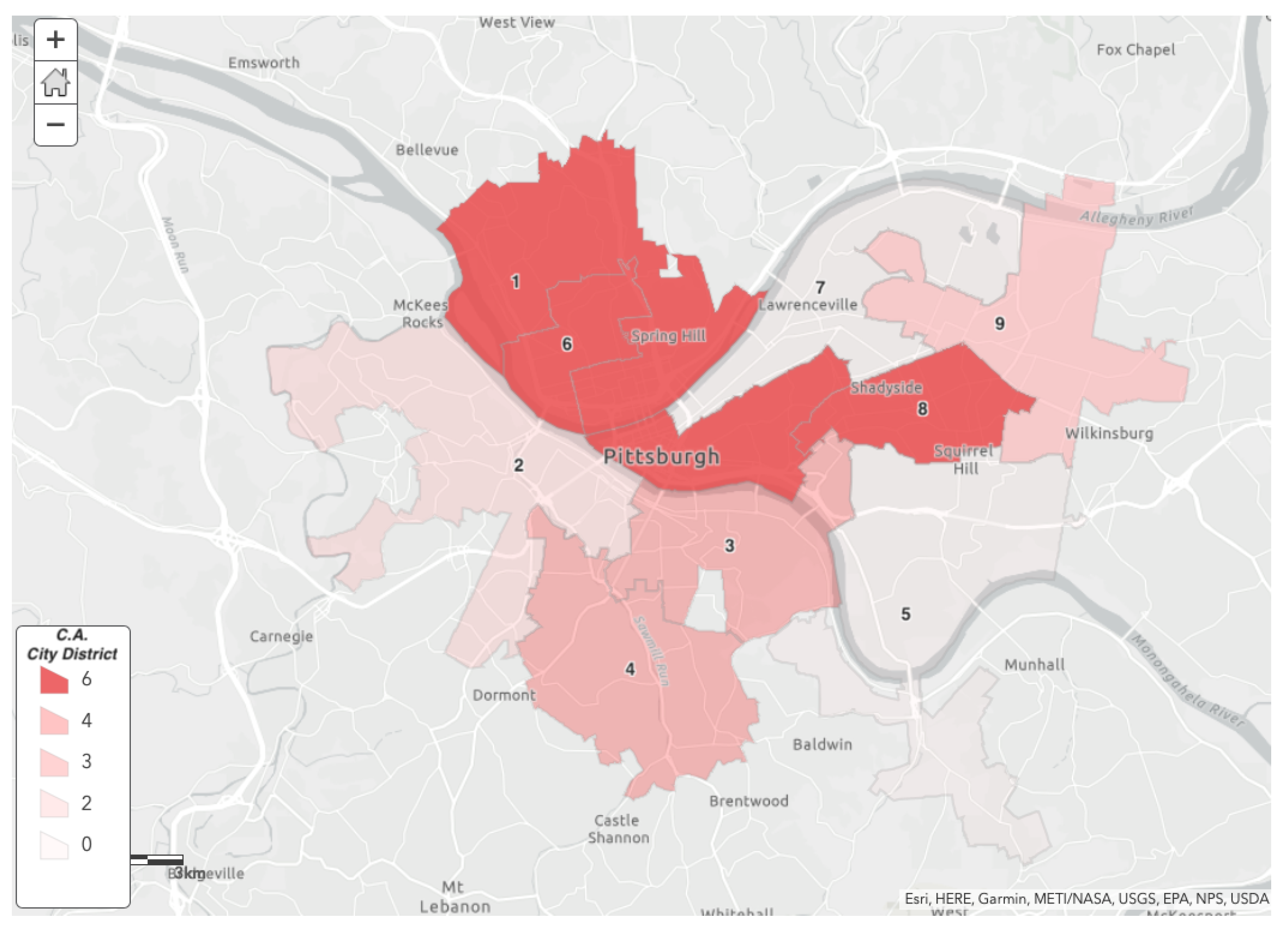
The City Council districts are developed based on political boundaries and serve as the legislative body in many US cities. For this case study, Pittsburgh consists of nine districts, and each covers several neighborhoods [27]. Figure 6 shows the value of the most critical districts in Pittsburgh city.
By comparing results from the above three geographical scale representations, we can conclude that there is an overlap of 50% between them, especially in the downtown area. According to feature selection, the number of nodes plays a high factor in determining the overall , and most of the downtown areas have large nodes. The exact reasons apply to other areas such as the Oakland and north shore areas.
By recognizing the critical geographical zones within the city scale, it becomes more accessible for the policymakers to leverage appropriate risk mitigating strategies such as security control for the critical region. Furthermore, this will intensify the overall resilience of interdependent critical infrastructure due to the complexity of the interdependent connectivity among them. Collecting the before-mentioned measures based on precise values such as critical nodes can develop in implementing the most reliable security control strategies to avoid future disaster events such as cascading failures. It can also assist in understanding the characteristics of the geographical territory, which presents us with the necessary information to enhance resilience in the critical infrastructures. Following the dependency and the complexity between essential nodes of infrastructure open the room for more tools to heighten all infrastructure resilience appearing in more sustained and resilient cities. However, just four central city-based infrastructures have been used in this work due to the data availability. The addition of more infrastructures will allow for more precise and accurate results. In addition, more measures will be added in the future to include other city aspects such as poverty and pandemics areas.
6. Conclusions
The criticality assessment methodology defined in this work extends the approach of Alqahtani et al. [19] by combining both graph centrality measures and dependency risk graphs as additional criteria for evaluating alternative critical geographical nodes strategies for interdependent critical infrastructures. The model aims to improve the preparedness phase resilience by assessing the critical zones of infrastructure, which allow for more space to adopt risk mitigation strategies. Future work can include applying more infrastructures and comparing the result with other cities or regions depending on the data availability and accuracy.
Author Contributions
Conceptualization, A.A. and D.T.; methodology, A.A.; software, A.A.; validation, A.A. and D.T.; formal analysis, A.A.; investigation, A.A.; resources, A.A.; data curation, A.A.; writing—original draft preparation, A.A.; writing—review and editing, A.A.; visualization, A.A.; supervision, D.T.; project administration, A.A. All authors have read and agreed to the published version of the manuscript.
Funding
This research received no external funding.
Data Availability Statement
Most of the data presented in the paper, including an additional and complete dataset, can be found at City Data Bank research data basis at (https://www.city-data.com) (Accessed: 20 July 2021) and United State Census Bureau at (https://www.UnitedStatesZipCodes.org) (Accessed: 20 July 2021).
Conflicts of Interest
The authors declare that they have no known competing financial interest or personal relationships that could have appeared to influence the work reported in this paper.
References
- Fisher, R.; Bassett, G.; Buehring, W.; Collins, M.; Dickinson, D.; Eaton, L.; Haffenden, R.; Hussar, N.; Klett, M.; Lawlor, M.; et al. Constructing a Resilience Index for the Enhanced Critical Infrastructure Protection Program; Technical Report; Argonne National Lab (ANL): Argonne, IL, USA, 2010. [Google Scholar]
- Nanab, C.; Sansavini, G.; Krögerc, W.; Heinimann, H. A quantitative method for assessing the resilience of infrastructure systems. In Proceedings of the PSAM 2014–Probabilistic Safety Assessment and Management, Berlin, Germany, 14–18 June 2014. [Google Scholar]
- Longstaff, P.H.; Armstrong, N.J.; Perrin, K.; Parker, W.M.; Hidek, M.A. Building resilient communities: A preliminary framework for assessment. Homel. Secur. Aff. 2010, 6, 1–23. [Google Scholar]
- Department of Homeland Security. Critical Infrastructure Sectors|Homeland Security. 2018. Available online: https://www.cisa.gov/critical-infrastructure-sectors (accessed on 20 July 2021).
- Eisenberg, D.A.; Park, J.; Seager, T.P. Sociotechnical network analysis for power grid resilience in South Korea. Complexity 2017, 2017, 3597010. [Google Scholar] [CrossRef] [Green Version]
- Stergiopoulos, G.; Kotzanikolaou, P.; Theocharidou, M.; Gritzalis, D. Risk mitigation strategies for critical infrastructures based on graph centrality analysis. Int. J. Crit. Infrastruct. Prot. 2015, 10, 34–44. [Google Scholar] [CrossRef]
- Wang, Z.; Ran, Z.; Chen, X.; Liang, Y.; Ren, Z.; He, Y. Critical Node Identification for Electric Power Communication Network Based on Topology and Services Characteristics. MATEC Web Conf. 2018, 246, 03023. [Google Scholar] [CrossRef]
- Gómez, J.F.; Martínez-Galán, P.; Guillén, A.J.; Crespo, A. Risk-Based Criticality for Network Utilities Asset Management. IEEE Trans. Netw. Serv. Manag. 2019, 16, 755–768. [Google Scholar] [CrossRef]
- Dick, K.; Russell, L.; Souley Dosso, Y.; Kwamena, F.; Green, J.R. Deep learning for critical infrastructure resilience. J. Infrastruct. Syst. 2019, 25, 05019003. [Google Scholar] [CrossRef]
- Van Bodegom, A.; Koopmanschap, E. The COVID-19 Pandemic and Climate Change Adaptation; Wageningen Centre for Development Innovation: Wageningen, The Netherlands, 2020; pp. 1–24. [Google Scholar]
- Alqahtani, A.; Tipper, D.; Kelly-Pitou, K. Locating Microgrids to Improve Smart City Resilience. In Proceedings of the Resilience Week 2018, RWS 2018, Denver, CO, USA, 20–23 August 2018. [Google Scholar] [CrossRef]
- Danielsson, P.E. Euclidean distance mapping. Comput. Graph. Image Process. 1980, 14, 227–248. [Google Scholar] [CrossRef] [Green Version]
- Patel, B. Producing reliable power in the hospital setting. Power Eng. 2011, 115, 20–24. [Google Scholar]
- Freeman, L.C. Centrality in social networks conceptual clarification. Soc. Netw. 1978, 1, 215–239. [Google Scholar] [CrossRef] [Green Version]
- Rinaldi, S.M. Modeling and simulating critical infrastructures and their interdependencies. In Proceedings of the Hawaii International Conference on System Sciences, Big Island, HI, USA, 5–8 January 2004. [Google Scholar] [CrossRef]
- Zio, E.; Sansavini, G. Modeling interdependent network systems for identifying cascade-safe operating margins. IEEE Trans. Reliab. 2011, 60, 94–101. [Google Scholar] [CrossRef] [Green Version]
- Ouyang, M.; Hong, L.; Mao, Z.J.; Yu, M.H.; Qi, F. A methodological approach to analyze vulnerability of interdependent infrastructures. Simul. Model. Pract. Theory 2009, 17, 817–828. [Google Scholar] [CrossRef]
- Kotzanikolaou, P.; Theoharidou, M.; Gritzalis, D. Assessing n-order dependencies between critical infrastructures. Int. J. Crit. Infrastruct. 6 2013, 9, 93–110. [Google Scholar] [CrossRef]
- Alqahtani, A.; Tipper, D.; Kelly-Pitou, K.; Amy, B. Identifying Vulnerable Critical Infrastructure Zones in Smart Cities. In Proceedings of the 2020 16th International Conference on the Design of Reliable Communication Networks DRCN 2020, Milan, Italy, 24–27 March 2020. [Google Scholar]
- Dodge, Y. The Oxford Dictionary of Statistical Terms; Oxford University Press: Oxford, UK, 2006. [Google Scholar]
- Bruce, P.; Bruce, A. Practical Statistics for Data Scientists: 50 Essential Concepts; O’Reilly Media, Inc.: Newton, MA, USA, 2017. [Google Scholar]
- Bottenberg, R.A.; Ward, J.H. Applied Multiple Linear Regression; 6570th Personnel Research Laboratory, Aerospace Medical Division, Air Force: Lackland Air Force Base, TX, USA, 1963; Volume 63. [Google Scholar]
- City-Data Bank. 2020. Available online: https://www.city-data.com (accessed on 19 July 2021).
- ESRI. ArcGIS Desktop: Release 10.2. 2013. Available online: https://www.esri.com (accessed on 20 July 2021).
- U.S. Census Bureau. Data Sources Include the United States Postal Service. 2020. Available online: https://www.unitedstateszipcodes.org (accessed on 20 July 2021).
- Jones, D.N. Defining City Neighborhoods an Imprecise Process. Pittsburgh-Post-Gaz 2020. Available online: https://www.google.com/url?sa=t&rct=j&q=&esrc=s&source=web&cd=&cad=rja&uact=8&ved=2ahUKEwjRnPq97Pz0AhWPohQKHVkJC3UQFnoECAwQAQ&url=https%3A%2F%2Fwww.post-gazette.com%2Flocal%2Fcity%2F2006%2F06%2F05%2FDefining-city-neighborhoods-an-imprecise-process%2Fstories%2F200606050129&usg=AOvVaw3ynvSPoTr2lFo9zV77AE6b (accessed on 20 July 2021).
- City Council, District Information, Neighborhoods. 2020. Available online: www.pittsburghpa.gov/council (accessed on 20 July 2021).
Figure 1.
Criticality Assessment Model.

Figure 2.
Network Modeling Showing The Interdependence Links Between Infrastructures.

Figure 3.
Dependency Risk Graph Between CIs Framework.

Figure 4.
Top Ten Critical Zip Code in Pittsburgh City.

Figure 5.
Most Critical Neighborhoods.

Figure 6.
Most Critical City Districts.


Table 1.
Likelihood Risk Dependence Matrix.
| Risk Dependence (i,j) | |||||
|---|---|---|---|---|---|
| VL | L | M | H | VH | |
| VL | 0–0.05 | 0–0.05 | 0–0.05 | 0–0.05 | 0–0.05 |
| L | 0–0.05 | 0.05–0.25 | 0.05–0.25 | 0.05–0.25 | 0.05–0.25 |
| M | 0–0.05 | 0.05–0.25 | 0.25–0.5 | 0.25–0.5 | 0.25–0.5 |
| H | 0–0.05 | 0.05–0.25 | 0.25–0.5 | 0.5–0.75 | 0.5–0.75 |
| VH | 0.05–0.25 | 0.05–0.25 | 0.25–0.5 | 0.5–0.75 | 0.75–1 |
Table 2.
Impact Risk Matrix.
| Risk Dependence (i,j) | |||||
|---|---|---|---|---|---|
| VL | L | M | H | VH | |
| VL | 1 | 2 | 3 | 4 | 5 |
| L | 2 | 3 | 4 | 5 | 6 |
| M | 3 | 4 | 5 | 6 | 7 |
| H | 4 | 5 | 6 | 7 | 8 |
| VH | 5 | 6 | 7 | 8 | 9 |
Table 3.
Centrality Measures.
| Zip Code | ||||
|---|---|---|---|---|
| 15211 | 13 | 6 | 0 | 0.90 |
| 15235 | 28 | 14 | 0 | 0.4 |
| 15106 | 8 | 24 | 0 | 0.28 |
| 15214 | 6 | 20 | 0 | 0.53 |
| 15216 | 13 | 38 | 11 | 0.20 |
| 15206 | 27 | 88 | 35 | 0.08 |
| 15217 | 23 | 82 | 18 | 0.11 |
| 15205 | 29 | 88 | 87 | 0.07 |
| 15203 | 13 | 40 | 26 | 0.18 |
| 15219 | 24 | 68 | 157 | 0.08 |
Table 4.
Interdependence Risk Graph based values.
| Sector | Zip Code | Coennected Nodes | Impact | Likehood | RD | C |
|---|---|---|---|---|---|---|
| communication | 15106 | 6 | 9 | 0.25 | 2.25 | 9.5 |
| Energy | 15106 | 5 | 6 | 0.5 | 3 | |
| Energy | 15106 | 5 | 6 | 0.5 | 3 | |
| Healthcare | 15106 | 2 | 1 | 0.25 | 0.25 | |
| Healthcare | 15106 | 2 | 1 | 0.25 | 0.25 | |
| Healthcare | 15106 | 2 | 1 | 0.25 | 0.25 | |
| Healthcare | 15106 | 2 | 1 | 0.25 | 0.25 | |
| Healthcare | 15106 | 2 | 1 | 0.25 | 0.25 |
Table 5.
Community Based Measures.
| Zip Code | ||||||
|---|---|---|---|---|---|---|
| 15206 | 9 | 215.5 | 2 | 31,216 | 24.65% | 2,861,972 |
| 15203 | 12 | 361.8 | 1 | 32,482 | 23.17% | 1,401,579 |
| 15210 | 3 | 172.5 | 3 | 28,320 | 29.10% | 1,890,664 |
| 15205 | 4 | 250.3 | 3 | 13,352 | 34.05% | 2,870,500 |
| 15208 | 4 | 183.5 | 4 | 31,850 | 23.82% | 1,052,736 |
| 15201 | 12 | 365.9 | 1 | 22,586 | 13.04% | 1,919,123 |
| 15216 | 4 | 114.8 | 4 | 19,204 | 34.50% | 1,656,714 |
| 15213 | 4 | 155.2 | 4 | 24,691 | 9.52% | 4,615,921 |
| 15219 | 16 | 86.0 | 1 | 1999 | 28.46% | 3,576,810 |
| 15120 | 6 | 593.8 | 2 | 9613 | 19.99% | 1,393,654 |
| 15222 | 16 | 74.1 | 1 | 29,621 | 8.61% | 2,897,465 |
Table 6.
Importance Level Corresponding To Each Measure.
| Feature | Importance | Measure | Importance |
|---|---|---|---|
| Number of Nodes | 1.178 | Criticality | 1.216 |
| Diversity of Nodes | 1.177 | ||
| Degree | 2.563 | Centrality | 1.614 |
| Betweeness | 2.861 | ||
| Closeness | 3.008 | ||
| Interdependence | - | Interdependence | 2.828 |
| Risk Value | 3.299 | Community | 1.156 |
| Electricity Use | 6.739 | ||
| Flooding Level | 3.355 | ||
| Population | 7.271 | ||
| Poverty Percent | 7.524 | ||
| Energy | 8.393 |
Publisher’s Note: MDPI stays neutral with regard to jurisdictional claims in published maps and institutional affiliations. |
© 2021 by the authors. Licensee MDPI, Basel, Switzerland. This article is an open access article distributed under the terms and conditions of the Creative Commons Attribution (CC BY) license (https://creativecommons.org/licenses/by/4.0/).
Share and Cite
MDPI and ACS Style
Almaleh, A.; Tipper, D. Risk-Based Criticality Assessment for Smart Critical Infrastructures. Infrastructures 2022, 7, 3. https://0-doi-org.brum.beds.ac.uk/10.3390/infrastructures7010003
AMA Style
Almaleh A, Tipper D. Risk-Based Criticality Assessment for Smart Critical Infrastructures. Infrastructures. 2022; 7(1):3. https://0-doi-org.brum.beds.ac.uk/10.3390/infrastructures7010003
Chicago/Turabian StyleAlmaleh, Abdulaziz, and David Tipper. 2022. "Risk-Based Criticality Assessment for Smart Critical Infrastructures" Infrastructures 7, no. 1: 3. https://0-doi-org.brum.beds.ac.uk/10.3390/infrastructures7010003