
A Geometric Classification of World Urban Road Networks
by
 , ,
, ,
Mohamed Badhrudeen
1, 
Sybil Derrible
1,*,
Trivik Verma
2,
Amirhassan Kermanshah
3 and
Angelo Furno
4 1
Department of Civil, Materials, and Environmental Engineering, University of Illinois, Chicago, IL 60607, USA
2
Department of Multi-Actor Systems, Faculty of Technology, Policy and Management, Delft University of Technology, 2628 BX Delft, The Netherlands
3
Department of Civil Engineering, Sharif University of Technology, Tehran 1458889694, Iran
4
LICIT UMR_T9401, University of Lyon, University Gustave Eiffel, ENTPE, 69675 Lyon, France
*
Author to whom correspondence should be addressed.
Urban Sci. 2022, 6(1), 11; https://0-doi-org.brum.beds.ac.uk/10.3390/urbansci6010011
Submission received: 20 January 2022
/
Revised: 5 February 2022
/
Accepted: 7 February 2022
/
Published: 11 February 2022
(This article belongs to the Special Issue The Implications of Human Mobility and Accessibility for Transportation and Livable Cities)
Abstract
:This article presents a method to uncover universal patterns and similarities in the urban road networks of the 80 most populated cities in the world. To that end, we used degree distribution, link length distribution, and intersection angle distribution as topological and geometric properties of road networks. Moreover, we used ISOMAP, a nonlinear dimension reduction technique, to better express variations across cities, and we used K-means to cluster cities. Overall, we uncovered one universal pattern between the number of nodes and links across all cities and identified five classes of cities. Gridiron Cities tend to have many 90° angles. Long Link Cities have a disproportionately high number of long links and include mostly Chinese cities that developed towards the end of the 20th century. Organic Cities tend to have short links and more non-90 and 180° angles; they also include relatively more historical cities. Hybrid Cities tend to have both short and long links; they include cities that evolved both historically and recently. Finally, Mixed Cities exhibit features from all other classes. These findings can help transport planners and policymakers identify peer cities that share similar characteristics and use their characteristics to craft tailored transport policies.

1. Introduction
Throughout history, cities have adapted to address the challenges they face [1]. In the early twenty-first century, urbanization, climate change, and resources constraints are some of the stressors that are forcing cities worldwide to reshape their urban infrastructure, often leveraging advances in technology [2]. Among the many urban infrastructure systems, transport infrastructure performs a critical role for a city to function properly. In many cities, transport infrastructure (both the physical infrastructure and infrastructure services) that has evolved sometimes over centuries or millennia now need to accommodate new urban travel dynamics and to address many challenges including traffic congestion and pollution related to transport activities. For example, the proliferation of ride hailing and micro mobility apps such as Lyft, Uber, Grab, and dockless scooter-share make it easier to travel to places that are not serviced by public transport. Further, micro mobility and ridesharing options (i.e., rides shared by multiple people) can reduce the cost of travel, making it attractive for short distance travel [3]. More generally, smart city initiatives are being widely deployed to address transport challenges. Smart city initiatives consist of policies aimed at managing and/or solving challenges, usually in a sustainable manner.
The core element of a smart city is leveraging technology, often thanks to the proliferation of large amounts of data that have become available, colloquially referred to as Big Data. In addition to improving how a transport system is operated, the influx of Big Data also provides an opportunity to better understand the current state of transport systems, notably through the definition and measure of indicators that characterize them. Indeed, every city has evolved over different timeframes and different time periods to address different challenges. Moreover, while some cities have grown organically (in the absence of a central force guiding urban network design) [4], others have been deliberately planned [5]. For example, a compendium of laws called “Laws of Indies” were used by Spanish settlers in designing their urban settlement [6]. During these processes, organic and deliberate planning or a mix of both, cities evolved with certain features unique to each. Gaining an understanding of the properties of transport systems can provide us with the ability to craft more effective solutions to address contemporary challenges. This study offers a method that leverages the availability of open-source maps and software to uncover the existence of universal patterns and similarities in urban road networks.
In this article, we focus on the spatial structure of transport road networks because their physical structure can play an important role on their overall performance [7] and in how cities are shaped [8,9]. Moreover, road networks have been studied to understand travel behavior [10,11,12], travel dynamics [13,14], public health [15,16], accessibility [17,18,19], and resilience [20,21,22,23] to name a few. More broadly, the physical structure of urban road networks can influence the performance in many different aspects of a city [24]. For instance, interruptions to any road links causes a connectivity loss; however, the degree of damage to the network varies depending on the properties of the interrupted links. In addition, road network properties can be used to identify the vulnerabilities in the networks, and to plan or improve their resilience [25,26,27]. Furthermore, characterizing and studying road networks across different cities can provide insights to further our understanding of urbanization and transport planning [28].
The main goal of this article is to propose a method that combines both topological and geometric information together to study and classify road network designs. The method was applied to the 80 most populated cities in the world. In terms of topological property, we used the degree distribution of the network. In terms of geometric property, we used both the distribution of link length and the distribution of street angles since they capture different properties of road networks. Combining these three pieces of information, we first sought the presence of universal patterns that exist in all networks. Second, we characterized road networks by discretizing the distribution of their properties, resulting in every urban road network being expressed by a single vector of variables. After applying ISOMAP (a dimensionality reduction technique), a clustering technique was employed to identify different classes of cities. Finally, we discuss the results and detail the characteristics of the classes found.
2. Network Science
Network Science is a discipline devoted to the study of networks [29,30] that has been heavily applied to study systems of all kinds [31,32], and in particular complex systems such as road systems [13,24,33,34,35,36,37,38,39,40,41,42,43]. Urban road networks are generally modelled as spatial and planar networks [44]. A spatial network is a network embedded within a 2D or 3D space and characterized by Euclidean geometry [45]. There has been a growing interest in studying urban roads as complex networks, partly fueled by advances in geographic information systems (GISs) and other new sources of information [44,45,46]. Past studies have shown, on a coarse grained level, the existence of similarities among different cities [44]. Characterizing urban road networks allows us to compare different cities and sometimes gain insights into their evolution and functional properties [47,48]. For example, considering road systems as networks, properties such as topological patterns, network efficiency, and network robustness can be studied and compared across cities. To find an accurate classification of cities based on road network properties, both topological and geometric properties should be considered [48]. Most past studies have studied single measures or a combination of multiple measures across different cities. For example, Boeing [49] studied the circuity of 40 different cities across the United States (US) and found that for most cities walking routes were less circuitous than driving routes. Similarly, Boeing [36] examined the network orientation and entropy of 100 cities; specifically, the study considered network’s bearings, entropy, and circuity to classify cities. The study used hierarchical clustering technique to classify cities and found three high-level and eight intermediate-level clusters.
In this article, each road system is represented as a network composed of nodes and links [50]. The nodes are the intersections formed by road segments and dead ends, and the links are the road segments themselves that connect the nodes. To quantitatively characterize the topological properties of road networks, various measures have been used in the literature, including network centrality measures such as betweenness centrality [13,27,34,37,51,52], closeness centrality [13,50,53,54,55], degree centrality [13,45,56,57,58,59] and clustering coefficient [35]. Each measure can be used to capture a certain property of the road networks. For example, betweenness centrality captures the ability to provide a path between regions in a network, and the betweenness centrality of a node is defined as the proportion of the network’s shortest paths going through the node [60]. Additional measures have been proposed and used by researchers. For instance, a new measure based on the block’s shape called “shape factor” was employed in [48] for the purpose of classifying cities. In this study, we used degree distribution (defined later) as the topological property of the network.
Beyond their topological properties, road systems also possess geometric properties. The most common geometric measure of road systems is link length [56]. For instance, Jiang [56] studied the transport networks of 40 cities in the US and concluded that the networks are not random and that they exhibit both small-world and scale-free properties. This conclusion was based on analyzing the degree distribution, path length, and clustering coefficient of the network of each city. Buhl et al. [47] considered both the geometric and topological elements of a road network to study its robustness and efficiency; in their study, the geometric element of the network considered was shortest path length. Albeit less common, angles created by intersections are another geometric measures used to study the geometry of road networks [24,61,62].
This study proposes a novel method that utilizes both topological and geometric properties of road networks to cluster cities with similar characteristics.
3. Materials and Methods
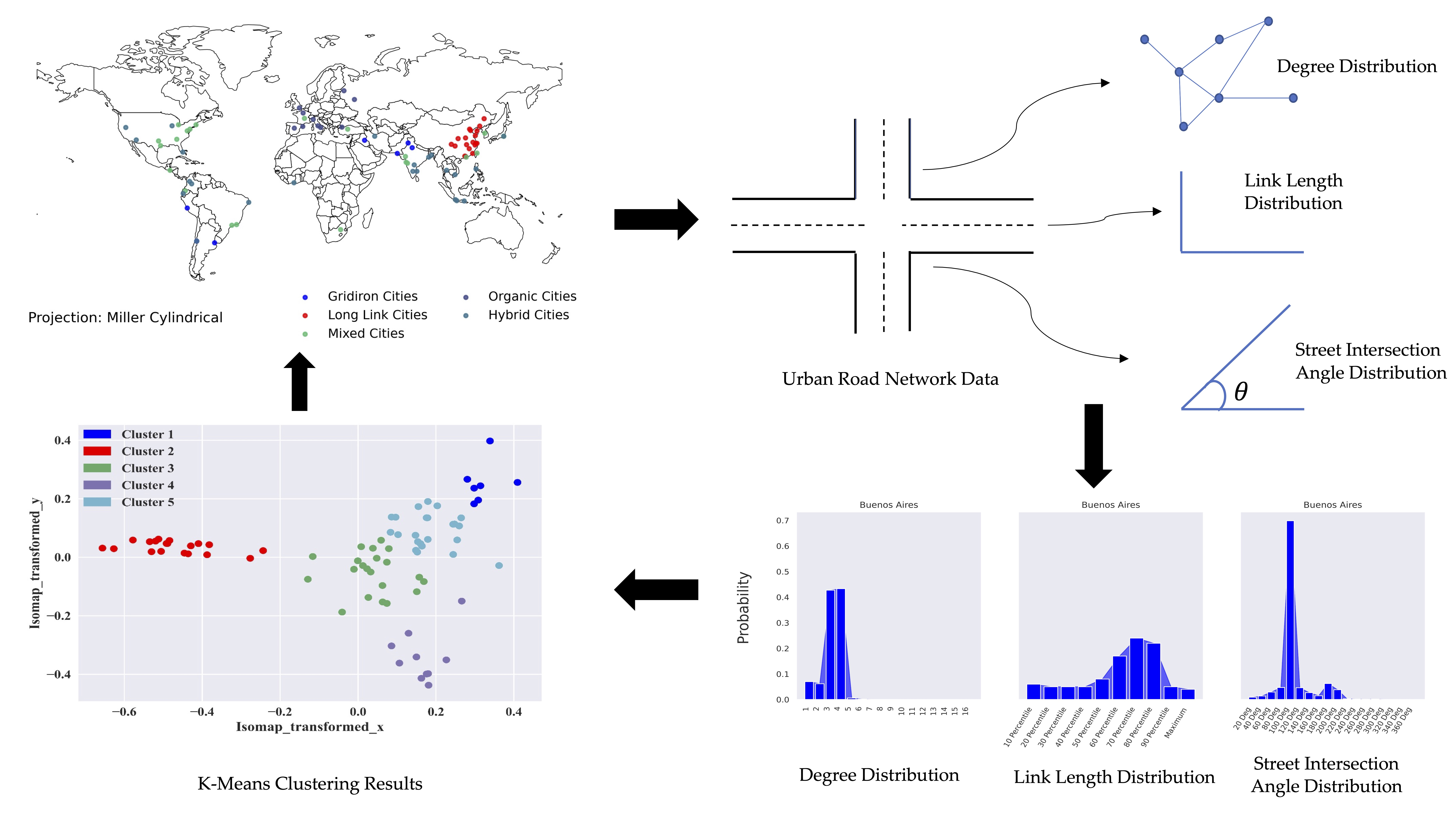
3.1. Data
This study utilizes the public data made available by Karduni et al. [63], who developed the open-sourced tool GIS Features 2 Edgelist (GISF2E) that converts any shapefile into a network. Further, Karduni et al. [63] applied the code to the road networks of 80 of the world’s most populated cities from OpenStreetMap (see a map in the Results section).
The extracted information includes the nodes and their geographical locations, and the length of each road segment (i.e., link length). The locations are in the form of Universal Transverse Mercator (UTM) coordinates and the link lengths are in meters. Additionally, information includes which nodes are connected by each link in the network. For example, if a network has a total of 100 links, the data will have 100 observations with each observation showing two nodes that are connected by that link, the nodes’ latitude and longitude coordinates, and the link’s length in meters. This information is enough to create a network.
3.2. Methodology
This study considers two main aspects of road systems: network topology and network geometry. Network topology captures the relationships between nodes through their links regardless of scale, as such it is mainly concerned with network connectivity. In contrast, network geometry is defined as the shape and magnitude of the connection between the nodes. One way to express network topology is by degree distribution. The degree distribution of an urban road network represents the distribution of its connections across the nodes. In this study, we only considered degree distribution as a measure of topological information since it is computationally easier to calculate (in contrast to other measures such as the distribution of betweenness centrality that tend to be highly correlated to degree distribution). To capture the network’s geometry, we considered link length and intersection angle. Link length is defined as the distance between two intersections (nodes). We used the intersection angle to identify whether the streets follow a planned pattern (e.g., a grid) or a more organic pattern. The three distributions used in this study are defined in this section as follows.
3.2.1. Degree Distribution
Firstly, in the context of urban road networks, a graph (G) is defined as a set of nodes or intersections N connected by links or road segments (L). Consider a graph G with N nodes and L Links, the degree distribution is the proportion of nodes with connections:
where is the adjacency matrix, in which the rows and columns represent the nodes in the network. The element is 1 if the node is connected to , or 0 if they are not connected. Then, the degree distribution is defined as:
where, is the total number of nodes with connections and N is the total number of nodes in the network. From all 80 cities, the variation in the distribution of degrees ranged from 1 (i.e., dead end) to 16. Nonetheless, 99.7% of the nodes have five or fewer connections.
3.2.2. Link Length Distribution
The link length distribution, , represents the probability that a road segment has a length . Link length distribution, however, is a continuous distribution, whereas we seek discrete values for clustering. A novelty of this work is that we fix different length categories (i.e., threshold values) based on the percentiles and the maximum value of the link length data of all 80 cities combined. Specifically, we considered the percentile categories of 10 to 90 with increments of 10. Once threshold percentile values from the 80 cities combined were found, we could construct an empirical link length distribution for every city individually by counting how many links belong to each bin. The bin limits are: length less than the 10th percentile from the 80 cities combined, between the 10th and 20th percentile, …, greater than the 90th percentile. As a result, the link length distribution of each city is turned into a discrete distribution of 10 values. Table 1 shows the threshold percentiles measured for link length distribution from the 80 cities combined.
3.2.3. Intersection Angle Distribution
The street’s intersection angle is the angle created when two road segments intersect. We calculated this angle information for each node that is connected to other nodes.
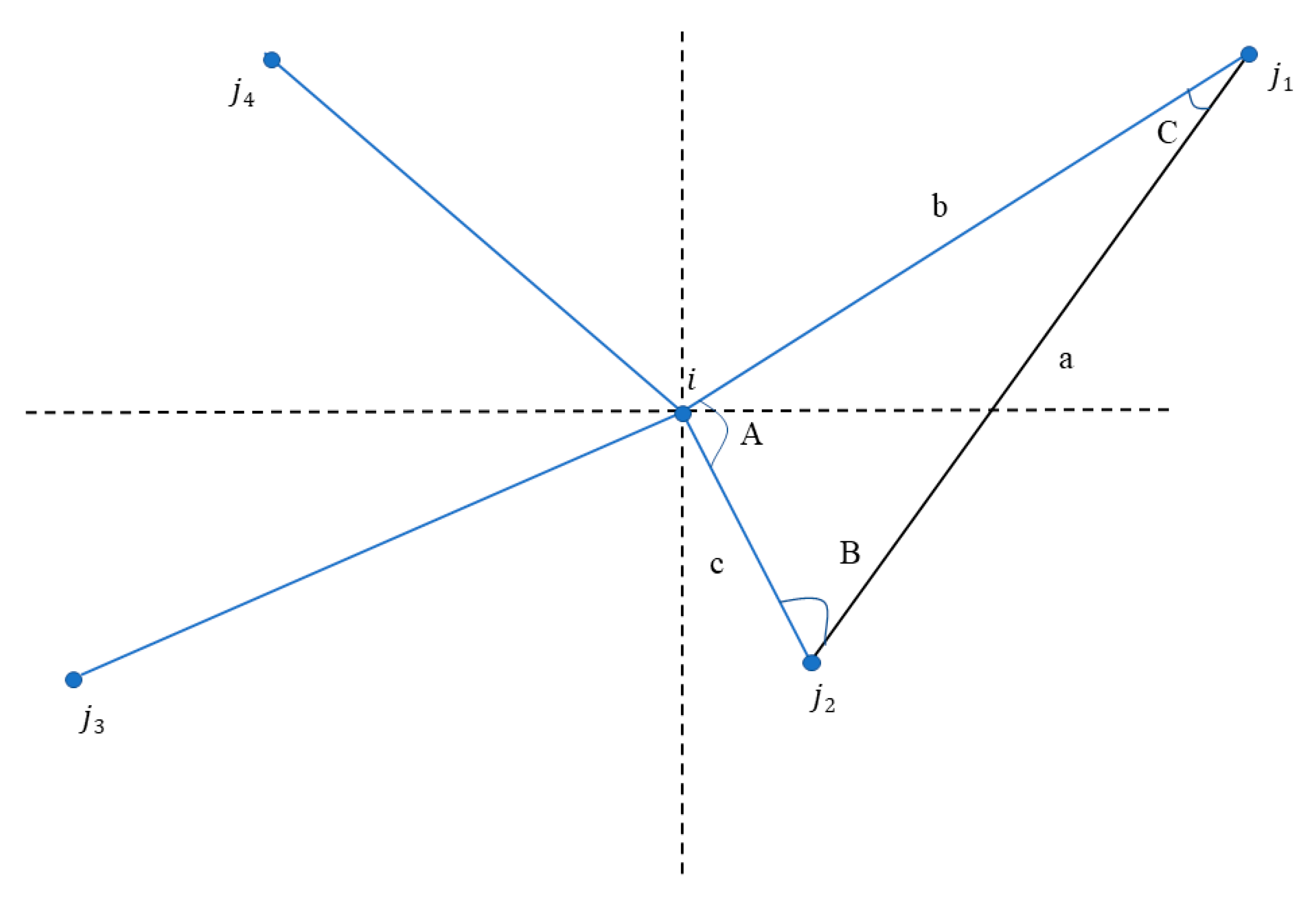
For example, as shown in Figure 1, if a node is directly connected to four other nodes, j1 to j4, then it creates four angles that sum to 360°. For a given node and its connected nodes , each angle is calculated for node and two nodes, e.g., and , that are adjacent to each other. As an example, consider the triangle to calculate the angle A shown in Figure 1. Since the information of latitudes and longitudes of the nodes , , and , and link lengths of and are known, we can calculate the distance between using the Haversine formula [64]. The angle is then calculated using the Cosine rule:
where are the sides of the triangle, and is the angle made by sides and . We repeated this procedure for all nodes. Similar to the link length distribution, the continuous distribution of street angles was discretized. Instead of using percentiles, a 20° bin size was selected, i.e., 0 to 20°, 20 to 40°, and so on, providing us probabilities of observing angles specific to each bin. For example, the probability of observing street angle between 80 and 100° in a city is, say 0.27. Overall, we have a vector with 18 values for each city, since there are 18 bins for 0 to 360° limit.
Finally, each city was expressed by a vector with 44 values (16 for degrees, 10 for link lengths, and 18 for street angles).
3.2.4. Clustering
We employed unsupervised machine learning methods to cluster cities based on their degree, link length, and street angle distributions information. Before that, however, we noted that the clustering entities based on 44 values (i.e., length of the vector measured for each city) representing three features of geometric and topological design is not necessarily meaningful. Because most clustering techniques utilize Euclidean distance measures to identify clusters, when the data dimension increases, the distance between data points in high dimensional space becomes more or less uniform [65]. Therefore, to better express the differences between cities, it is often preferable to reduce the dimensionality of the vector used while preserving the inherent features of the road networks. For this, we first transformed the raw data using ISOMAP [66], which is a non-linear dimensionality reduction technique. ISOMAP was selected thanks to its ability to preserve the variation in the original data in the transformed data. Additionally, since the data are probability distributions, any nonlinear behavior would not be captured by linear dimensionality reduction techniques such as Principal Component Analysis (PCA).
The ISOMAP algorithm finds the data points that are closer to each other (neighbors) based on the distance between data points . Two methods are usually used to find the neighbors: (1) k nearest neighbors (knn) or (2) a fixed radius. Both require a parameter defined by the user; knn requires the number of data points as neighbors (5 was selected), and fixed radius requires the selection of a pre-determined radius ε within which all nodes will be considered as neighbors. Then, it forms a graph H where all data points that are identified as neighbors are connected to each other. The data points in the graph H are a subset of the whole data; the subset space is considered to be Euclidean. In the second step, the algorithm calculates the shortest path distance of graph H between all pairs of data points. The idea is to break down the whole dataset into multiple subsets so that the geodesic distance inherent to the data projected onto an unknown manifold space is preserved. In the algorithm’s context, the geodesic distance is defined as the shortest distance between two points along the manifold space which is locally Euclidean. For example, let us consider the whole dataset has been broken down into 20 subsets (graphs), as such . The shortest path between two points, say, one in subset 1 and another in subset 20, would be the summation of all shortest paths observed in subsets H. This yields a square matrix . Finally, the algorithm constructs a low dimensional Euclidean space (Y), for instance a 2-D space, to embed the data that preserve the distance of the original data. For each point , the coordinates , which is a vector consisting of in space Y (2D), were chosen in such a way to minimize the following cost function [66]:
where , is the Euclidean distance matrix between all pairs of data points in space Y, is the norm of the matrix, and is the operator that converts the distances to inner products for efficient optimization. Using ISOMAP, raw data that consist of 44 vectors can be transformed to two dimensional vectors.
We then compared the performances of several clustering techniques on the resulting two-dimensional vector, including K-means [67], spectral clustering [68], hierarchical clustering [69], and HDBSCAN [70], and assessed them based on their silhouette score [71] (see Table 2). All these clustering algorithms work based on the Euclidean distance between data points.
Based on the silhouette scores calculated (presented later in the results section) for different clustering techniques, K-means clustering was selected as the preferred method. K-means clustering is an iterative procedure that essentially minimizes the distance between a cluster’s centroid to its data points. The centroid of a cluster is simply a coordinate of the center of a cluster.
First, given clusters with centroids , for each cluster , a centroid is arbitrarily chosen, and the data points closer to the centroid are assigned to the cluster based on the minimization of the function, . After the end of the first iteration, the centroids are updated by taking the mean of all data points in each cluster; as:
The procedure was then repeated assigning data points to the closest cluster. The centroids were then updated again, and so on, until all data points were assigned to a fixed cluster.
4. Results
4.1. Universal Pattern
A preliminary analysis reveals that the nodes and the links for all the 80 cities possess a linear relationship of the form, . Figure 2 shows the linear fit. We found the R2 value of 0.99 for this fit. This result suggests the presence of a universal mechanism that directs the road network growth. In other words, this relationship shows that on average each node is connected to 1.33 links, and this trend is found to be universally true for all cities regardless of when the road network was developed.
Moreover, unlike many urban properties that follow sublinear and super-linear scaling laws [72], this value stays constant regardless of the size of the network. In other words, a large network follows the same pattern as a small network, likely due to the spatial feature of road systems.
4.2. Road Network Analysis
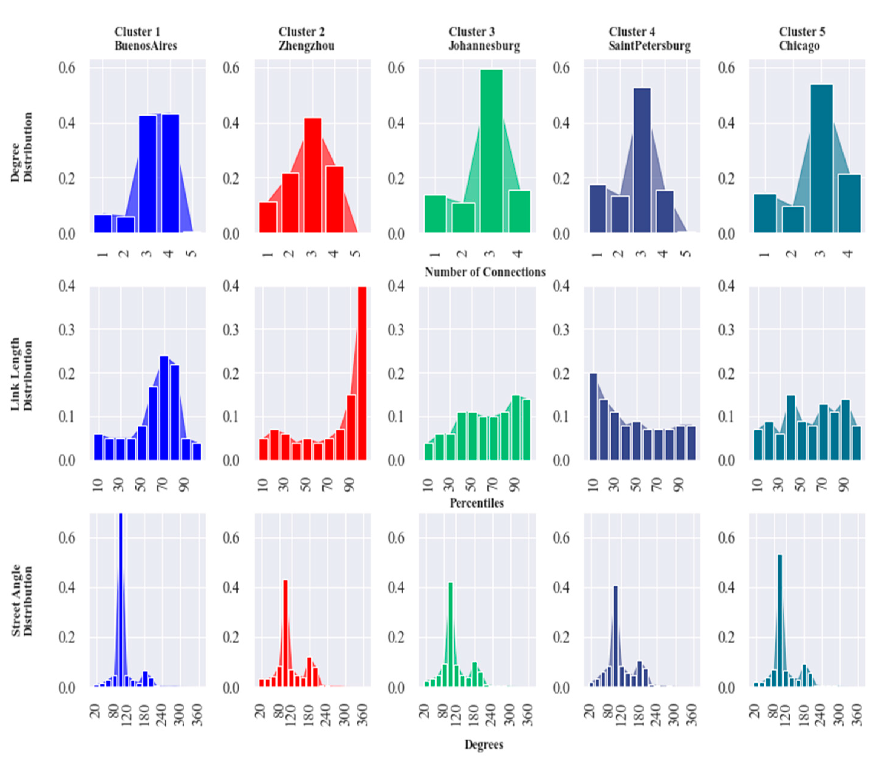
Figure 3 shows the three distributions for five representative cities from each class (discussed later). Starting with degree distribution, the most frequent degree across all cities is 3; i.e., a T-shaped intersection. This observation is in line with results showed by Lee and Jung [73]. The authors analyzed the streets patterns in 22 Korean cities and found that streets with three connections were more frequent than streets with four connections. In our study, the only exception is Buenos Aires where many intersections also have a degree of 4, which is a manifestation of heavy deliberate planning, strictly following a grid pattern for streets.
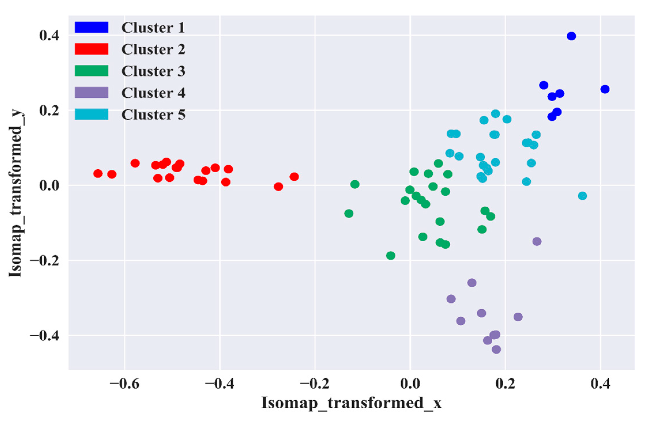
Figure 4.
Plot of clustered cities using ISOMAP and K-means clustering.

The link length distributions show that some cities have more long links than short links, while other cities, in contrast, have more short links than long links. Looking at Buenos Aires, we observe more link lengths that are greater than the 50th percentile and less than the 80th percentile compared with other categories.
From the street intersection angle distribution, we found that all cities exhibit a similar pattern. The distributions are clearly bimodal with peaks occurring at angles of 90 and 180°. Looking at the street angle distribution, again Buenos Aires has higher percentage of 90° angles compared with other cities since it has more intersections of degree 4 (i.e., four 90° angles) compared with all other cities that have more intersections of degree 3 (i.e., two 90° angles and one 180° angle). The distributions of all 80 cities studied are shown in the Supplementary Materials.
As described above, we tested several clustering algorithms and used the silhouette score to assess their performance (see Table 2). We adopted a two-step process. In the first step, we tested the performance of four clustering techniques, namely, K-Means, Spectral K-Means, Hierarchical, and HDBSCAN. The best clustering technique was picked based on the highest silhouette score. The analysis showed that the K-means clustering technique outperformed the other techniques; hence it was ultimately selected. In the second step, we used two measures to find the optimal number of clusters: the silhouette score and the sum of squared distance. Based on these two measures, we found the optimal number of clusters to be 5; the full results of the second step are provided in the Supplementary File.
The results of the K-means clustering technique is shown in Figure 4 where clusters are plotted using the resultant two vectors from ISOMAP. The list of cities per group is shown in Table 3. By looking into the properties of cities present in each cluster, we can establish a classification of world urban road networks.
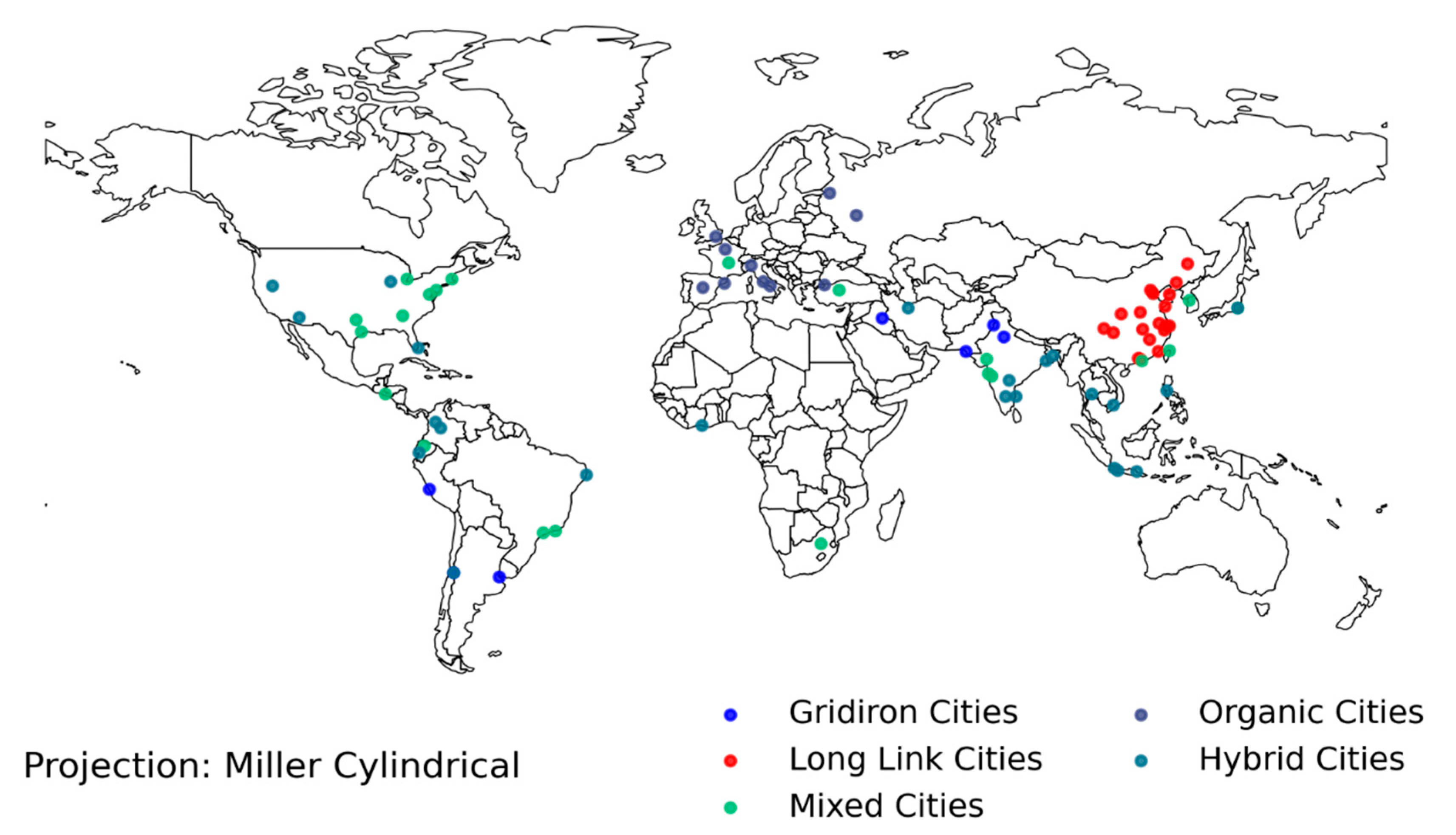
Figure 5.
Different classes of cities projected onto a world map.

5. Discussion
5.1. Cities Classification
Figure 5 shows a map of all cities colored coded based on their class. Cities in class 1 are referred to as Gridiron Cities since they are characterized by having comparatively more 90° angles than cities in other classes. These kind of cities typically are the result of deliberate planning practices, aiming to achieve an “efficient flow of traffic” [73]. Furthermore, cities in class 1 tend to have as many nodes with one connection as nodes with two connections. Generally, the grid layout or orthogonal layout tend to have an intersection angle of 90° and/or 180°. For example, Buenos Aires, which is one of the deliberately planned cities, exhibits the grid layout, and has equal number of nodes with three and four connections. Grid layouts, in most cases, result in square or rectangular block shapes. This also aligns with the conclusion provided by Louf and Barthelemy [74] that Buenos Aires consists predominantly of square or rectangular blocks. Moreover, other Latin American cities, namely Lima and Santiago, are also found to belong to the Gridiron Cities class (perhaps as a result of the “Laws of Indies” mentioned above). Despite having evolved over millennia, Baghdad also belongs to class 1 since it evolved significantly in the 1960s, following modern planning practices; hence the rise to more “rigid rectilinear grid systems of roads, and highways” [75].
Cities in class 2 consist predominantly of Chinese cities that have grown substantially at the turn of the 21st century and that are characterized by longer link lengths (i.e., large block size). They are referred to as Long Link Cities. In other words, link lengths greater than 90th percentile are more prevalent in these cities. This type of “leapfrog development” is common in the urban development of many Chinese cities [76]. Specifically, leapfrog development is characterized by developers skipping large areas to acquire cheaper lands further away, resulting in a form of urban sprawl. Overtime, this type of development practice generally causes polycentricity [77]. LOBsang et al. [55] studied 31 Chinese cities to understand the relationship between their street network properties and economic development. In their study, the authors identified that many cities with longer street length were polycentric. While this study focuses purely on Chinese cities, a similar study by Wang et al. [78] compared the Chinese city of Xiamen with Washington DC and San Jose, and found that the average road segment length of Xiamen is greater than the other two American cities. In our study, we also found most of the Chinese cities have more nodes with two connections than nodes with one connection.
Cities in class 3 are mainly comprised of radial cities that have developed over many centuries, often organically. They are referred to as Organic Cities. Unlike Gridiron Cities, these cities did not evolve by continuous directed planning. Instead, they evolved by adapting to local circumstances such as wars throughout history. We found cities in this class were characterized by shorter link lengths and a higher proportion of irregular street patterns (i.e., street angles that are not 90 or 180°). All the cities in this class are European cities, echoing the results of other studies. For instance, Strano et al. [50] studied 10 European cities and showed that they share common structural geometric properties. The authors also showed that all those 10 cities had shorter link lengths. Liu and Jiang [79] compared three European cities with three North American cities and showed the European cities have more short street segments and irregular street patterns. Further, Kaoru et al. [80] studied the road network of 30 European cities and identified similarities in spatial distribution of road segments at a larger scale (more than 1 km radius).
Cities in class 4 are characterized by a uniform distribution of link lengths and a higher proportion of 90° angles. They are referred to as Hybrid Cities. Many of the cities present in class 4 have evolved both historically and recently. The city of Chicago and the many municipalities around Chicago, for example, grew substantially in the second half of the 19th century, before the advent of the private automobile, hence the presence of many shorter links. As the region continued to grow in the 20th century, longer links were built to link these municipalities, eventually leading urban sprawl, hence the almost uniform distribution in link length. A similar observation was made by Lee and Jung [73] who found that the core area of the cities exhibit urban characteristics, whereas the outer areas exhibit rural characteristics. The authors define urban characteristics as the concentration of “density of the roads and intersections” in the central area, and less dense in the rural (outer) areas. Therefore, Hybrid Cities can be viewed as cities that have both structural properties of urban and rural streets.
Cities in class 5 contain a mix of characteristics from the other classes. Cities are the results of long term evolution and are influenced by multiple factors including social, economic, environmental, and landscapes [81]. The growing process is also dynamic with new roads being paved to access already established places such as city centers and spreads outwards [82]. Thus, in general many cities share similarities, particularly cities with similar social, economic, and landscape features. This fact is further exhibited in Figure 4 as cities in class 5 are physically located in the center of the figure (shown in green). Therefore, cities in class 5 have both some shorter links and some longer links. They also have a non-negligible number of street angles that are not 90 or 180°. These cities are referred to as Mixed Cities as they possess mixed characteristics.
5.2. Research and Policy Implications
The implications of this study are that the proposed methodology can be helpful to both transport planners and policymakers in identifying structurally similar cities. The geometry and topology of road networks are known to impact network performance. Yet, despite the presence of correlations between network properties and performance, the underlying factors that contribute to it are underexplored [83]. Historically, designing road networks included altering existing networks or adding new roads without taking their impacts on the whole network into account [84]. Such alterations are generally carried out to achieve a particular outcome; for example, to improve traffic congestion or promote active transport. For instance, in the 1950s and 1960s, the private vehicle was often seen as a potential solution to many transport problems [85]. This idea was reflected in their design: longer links, grid layouts, and so on. Identifying cities that are structurally similar can allow transport planners to find cities in their cluster that have better performance.
Furthermore, the classes identified in this study can be used to study urban design principles that can be adopted/replicated by transport planners. For example, analyzing traffic accident patterns in each class may help transport planners identify important causal variables for transport safety analysis. Additionally, in active transport, cities such as Amsterdam, Copenhagen, and Lund are considered frontrunners in Europe [85]. Finding in which class these cities belong can inform transport planners on the role of road network properties in recommending active transport policies. Therefore, gaining an understanding of the characteristics of the road network of a city is important to be able to develop effective design practices and select appropriate policies to address urban challenges. In addition, the methodology presented in this study can help policymakers to identify already implemented smart city policies in different cities that share structural road network similarities.
Furthermore, many cities in low- and middle-income countries might not have the necessary resources to experiment in the pursuit of smart city development. As a result, cities can look toward their peer cities to learn insights that can make them “smarter” [86]. Further, cities often have urban problems that are similar to their peers and learning urban practices from their peers can improve the understanding of what works and what does not [87]. Hodgkinson [88] argues that cities turning towards their peers create opportunities to learn and “[share] insights, ideas, and solutions.” However, it is rarely practiced partly because of the lack of “global inter-urban perspective” in smart city development [89]. The methodology proposed in this study offers a way to select structurally similar peer cities. Based on this work, we posit that smart transport policies implemented in cities of one class may not be as effective as in cities of another class. For instance, Guo et al. [90] found that the same smart city policy towards improving traffic congestion did not yield the same improvements across different cities in China. Although the authors stated the significance of road networks in analyzing traffic congestion, the road networks information was not included in their study. Moreover, the authors highlighted the lack of methodologies that can accurately classify cities based on road networks. We note that further investigation is required to assess the performance of cities in each class. Investigating this question and defining and assessing the performance of a specific road network structure is the goal of future work.
6. Conclusions
The geometric and topological characteristics of urban road networks can play an important role in shaping their performance and the travel behavior of city residents. Using geometric and topological data, this article classified the urban road networks of 80 world cities. Degree distribution was used as a measure of network topology, and link length distribution and street angle distribution were used as measures of network geometry. An initial analysis showed the presence of a universal pattern expressed by a clear linear relationship between the number of nodes and the number links across all cities present in the dataset. It further showed that an average 1.33 links was observed for every node in the network regardless of the size of the network. To successfully cluster urban road networks, the vector with 44 values measured for each city was transformed with ISOMAP to reduce the number of dimensions to 2 to meaningfully express the variation in the data and improve clustering performance. From the different clustering algorithms tested, K-means clustering performed best based on silhouette score. We found through further analysis that the optimal number of clusters was five, that is, we found five classes of cities.
Class 1 consists of Gridiron Cities that show a higher number of 90° street angles. Class 2 consists mostly of Chinese cities. The cities have a higher percentage of longer link lengths than any other cities considered in this study and were named Long Links Cities. Cities in class 3, named Organic Cities, were comprised mostly of radial cities such as Paris, Rome, and Madrid; these cities have shorter links and many non-90 and 180° angles. Class 4 cities, named Hybrid Cities, includes cities that have evolved both historically and recently; these cities tend to have a uniform distribution of link lengths and a higher proportion of 90° angles. Cities in class 5 exhibit a mix of properties from all other classes. Cities in this class have both some shorter links and some longer links, and they also have a non-negligible number of street angles that are not 90 or 180°, thus they are named Mixed Cities.
The findings of our study shows that there is a clear difference in the topological and geometric properties of road networks between classes of cities. Identifying these characteristics among cities can help transport planners to improve the performance of transport systems. Further, the findings may help policymakers in developing transport policies that are appropriate to cities based on the characteristic of their class. The impacts of road network characteristics, however, on the successful execution of transport policies, especially urban mobility policies, need further research. Future work should focus on studying the impacts of the network characteristics identified on the performance of a road system. Eventually, understanding the road network characteristics of a city can be helpful in developing transport policies and in improving the design of existing transport networks to meet contemporary challenges.
Supplementary Materials
The following supporting information can be downloaded at: https://0-www-mdpi-com.brum.beds.ac.uk/article/10.3390/urbansci6010011/s1, Figure S1: Degree distribution of all 80 Cities, Figure S2: Link Length distribution of all 80 Cities, Figure S3: Street intersection angle distribution of all 80 Cities, Figure S4: Silhouette score measure to find optimal number of clusters, Figure S5: Sum of squared distance measure to find optimal number of clusters.
Author Contributions
Conceptualization, S.D. and M.B.; methodology, M.B. and S.D.; coding, M.B.; formal analysis, M.B.; investigation, M.B., S.D. and T.V.; resources, S.D.; data curation, A.K.; writing—original draft preparation, M.B. and S.D.; writing—review and editing, M.B., S.D., T.V., A.K. and A.F.; visualization, M.B.; funding acquisition, S.D. All authors have read and agreed to the published version of the manuscript.
Funding
This research is supported, in part, by the National Science Foundation (NSF) CAREER Award [1551731].
Institutional Review Board Statement
Not applicable.
Informed Consent Statement
Not applicable.
Data Availability Statement
The data used in this study is freely available [63] and can be found at https:figshare.com/articles/dataset/Urban_Road_Network_Data/2061897 (accessed on 9 February 2022).
Conflicts of Interest
The authors declare no conflict of interest.
References
- Derrible, S. Complexity in future cities: The rise of networked infrastructure. Int. J. Urban Sci. 2017, 21, 68–86. [Google Scholar] [CrossRef]
- Derrible, S. Urban Engineering for Sustainability; The MIT Press: Cambridge, MA, USA, 2019; Available online: https://mitpress.mit.edu/books/urban-engineering-sustainability (accessed on 11 May 2021).
- McKenzie, G. Urban mobility in the sharing economy: A spatiotemporal comparison of shared mobility services. Comput. Environ. Urban Syst. 2020, 79, 101418. [Google Scholar] [CrossRef]
- Batty, M.; Marshall, S. Thinking organic, acting civic: The paradox of planning for Cities in Evolution. Landsc. Urban Plan. 2017, 166, 4–14. [Google Scholar] [CrossRef]
- Barthelemy, M.; Bordin, P.; Berestycki, H.; Gribaudi, M. Self-organization versus top-down planning in the evolution of a city. Sci. Rep. 2013, 3, 2153. [Google Scholar] [CrossRef] [PubMed] [Green Version]
- Martínez-Mendoza, R. Analyzing Urban Spaces: A Comparative Study of Sociability in Two Plazas in Santiago de Querétaro City, Mexico. 2001. Available online: https://ttu-ir.tdl.org/handle/2346/61606 (accessed on 20 October 2021).
- Amini, B.; Peiravian, F.; Mojarradi, M.; Derrible, S. Comparative Analysis of Traffic Performance of Urban Transportation Systems. Transp. Res. Rec. J. Transp. Res. Board 2016, 2594, 159–168. [Google Scholar] [CrossRef]
- Derrible, S. An approach to designing sustainable urban infrastructure. MRS Energy Sustain. 2018, 5, E15. [Google Scholar] [CrossRef] [Green Version]
- Marshall, S. Streets and Patterns; Routledge: London, UK, 2004; p. 328. ISBN 978-1-134-37075-7. [Google Scholar]
- Cervero, R.; Kockelman, K. Travel demand and the 3Ds: Density, diversity, and design. Transp. Res. Part D Transp. Environ. 1997, 2, 199–219. [Google Scholar] [CrossRef]
- Handy, S.L.; Boarnet, M.G.; Ewing, R.; Killingsworth, R.E. How the built environment affects physical activity: Views from urban planning. Am. J. Prev. Med. 2002, 23, 64–73. [Google Scholar] [CrossRef]
- Uchida, K. Estimating the value of travel time and of travel time reliability in road networks. Transp. Res. Part B Methodol. 2014, 66, 129–147. [Google Scholar] [CrossRef]
- Lin, J.; Ban, Y. Comparative Analysis on Topological Structures of Urban Street Networks. ISPRS Int. J. Geo-Inf. 2017, 6, 295. [Google Scholar] [CrossRef] [Green Version]
- Akbarzadeh, M.; Memarmontazerin, S.; Derrible, S.; Salehi Reihani, S.F. The role of travel demand and network centrality on the connectivity and resilience of an urban street system. Transportation 2019, 46, 1127–1141. [Google Scholar] [CrossRef]
- Marshall, W.E.; Piatkowski, D.P.; Garrick, N.W. Community design, street networks, and public health. J. Transp. Health 2014, 1, 326–340. [Google Scholar] [CrossRef]
- Frizzelle, B.G.; Evenson, K.R.; Rodriguez, D.A.; Laraia, B.A. The importance of accurate road data for spatial applications in public health: Customizing a road network. Int. J. Health Geogr. 2009, 8, 24. [Google Scholar] [CrossRef] [PubMed] [Green Version]
- Taylor, M.A.P.; Sekhar, S.V.C.; D’Este, G.M. Application of Accessibility Based Methods for Vulnerability Analysis of Strategic Road Networks. Netw. Spat. Econ. 2006, 6, 267–291. [Google Scholar] [CrossRef]
- Taylor, M.A.P. Susilawati Remoteness and accessibility in the vulnerability analysis of regional road networks. Transp. Res. Part A Policy Pract. 2012, 46, 761–771. [Google Scholar] [CrossRef]
- Fancello, G.; Carta, M.; Fadda, P. A Modeling Tool for Measuring the Performance of Urban Road Networks. Procedia Soc. Behav. Sci. 2014, 111, 559–566. [Google Scholar] [CrossRef] [Green Version]
- Zhang, W.; Wang, N. Resilience-based risk mitigation for road networks. Struct. Saf. 2016, 62, 57–65. [Google Scholar] [CrossRef] [Green Version]
- Wang, J. Resilience of Self-Organised and Top-Down Planned Cities—A Case Study on London and Beijing Street Networks. PLoS ONE 2015, 10, e0141736. [Google Scholar] [CrossRef]
- Sharifi, A. Resilient urban forms: A review of literature on streets and street networks. Build. Environ. 2019, 147, 171–187. [Google Scholar] [CrossRef]
- Kermanshah, A.; Derrible, S.; Berkelhammer, M. Using Climate Models to Estimate Urban Vulnerability to Flash Floods. J. Appl. Meteorol. Climatol. 2017, 56, 2637–2650. [Google Scholar] [CrossRef]
- Xie, F.; Levinson, D. Measuring the Structure of Road Networks. Geogr. Anal. 2007, 39, 336–356. [Google Scholar] [CrossRef]
- Sharifi, A. A typology of smart city assessment tools and indicator sets. Sustain. Cities Soc. 2020, 53, 101936. [Google Scholar] [CrossRef]
- Gauthier, P.; Furno, A.; El Faouzi, N.-E. Road Network Resilience: How to Identify Critical Links Subject to Day-to-Day Disruptions. Transp. Res. Rec. 2018, 2672, 54–65. [Google Scholar] [CrossRef] [Green Version]
- Henry, E.; Furno, A.; Faouzi, N.-E.E. Approach to Quantify the Impact of Disruptions on Traffic Conditions using Dynamic Weighted Resilience Metrics of Transport Networks. Transp. Res. Rec. 2021, 2675, 61–78. [Google Scholar] [CrossRef]
- Boeing, G. Street Network Models and Indicators for Every Urban Area in the World. Geogr. Anal. 2021. Available online: https://0-onlinelibrary-wiley-com.brum.beds.ac.uk/doi/abs/10.1111/gean.12281 (accessed on 9 March 2021). [CrossRef]
- Newman, M. Networks: An Introduction; Oxford University Press: Oxford, UK, 2010; p. 789. ISBN 978-0-19-920665-0. [Google Scholar]
- Barabási, A.-L.; Pósfai, M. Network Science; Cambridge University Press: Cambridge, UK, 2016; p. 477. ISBN 978-1-107-07626-6. [Google Scholar]
- Ahmad, N.; Derrible, S. Evolution of Public Supply Water Withdrawal in the USA: A Network Approach. J. Ind. Ecol. 2015, 19, 321–330. [Google Scholar] [CrossRef]
- Derrible, S.; Ahmad, N. Network-Based and Binless Frequency Analyses. PLoS ONE 2015, 10, e0142108. [Google Scholar] [CrossRef]
- Chalasani, V.S.; Denstadli, J.M.; Engebretsen, O.; Axhausen, K.W. Precision of geocoded locations and network distance estimations. J. Transp. Stat. 2005, 8, 1–15. [Google Scholar]
- Crucitti, P.; Latora, V.; Porta, S. Centrality measures in spatial networks of urban streets. Phys. Rev. E 2006, 73, 036125. [Google Scholar] [CrossRef] [Green Version]
- Jiang, B.; Claramunt, C. Topological Analysis of Urban Street Networks. Environ. Plan. B Plan. Des. 2004, 31, 151–162. [Google Scholar] [CrossRef] [Green Version]
- Boeing, G. Urban spatial order: Street network orientation, configuration, and entropy. Appl. Netw. Sci. 2019, 4, 67. [Google Scholar] [CrossRef] [Green Version]
- Akbarzadeh, M.; Memarmontazerin, S.; Soleimani, S. Where to look for power Laws in urban road networks? Appl. Netw. Sci. 2018, 3, 4. [Google Scholar] [CrossRef] [Green Version]
- Tsiotas, D.; Polyzos, S. The topology of urban road networks and its role to urban mobility. Transp. Res. Procedia 2017, 24, 482–490. [Google Scholar] [CrossRef]
- Dumedah, G.; Garsonu, E.K. Characterising the structural pattern of urban road networks in Ghana using geometric and topological measures. Geo Geogr. Environ. 2021, 8, e00095. [Google Scholar] [CrossRef]
- Martínez Mori, J.C.; Samaranayake, S. Bounded Asymmetry in Road Networks. Sci. Rep. 2019, 9, 11951. [Google Scholar] [CrossRef]
- Boeing, G. OSMnx: New methods for acquiring, constructing, analyzing, and visualizing complex street networks. Comput. Environ. Urban Syst. 2017, 65, 126–139. [Google Scholar] [CrossRef] [Green Version]
- Hillier, W.R.G.; Turner, A.; Yang, T.; Park, H. Metric and topo-geometric properties of urban street networks: Some convergencies, divergencies and new results. J. Space Syntax 2010, 1, 258–279. [Google Scholar]
- Nicosia, V.; Criado, R.; Romance, M.; Russo, G.; Latora, V. Controlling centrality in complex networks. Sci. Rep. 2012, 2, 218. [Google Scholar] [CrossRef] [PubMed] [Green Version]
- Barthélemy, M. Spatial networks. Phys. Rep. 2011, 499, 1–101. [Google Scholar] [CrossRef] [Green Version]
- Merchán, D.; Winkenbach, M.; Snoeck, A. Quantifying the impact of urban road networks on the efficiency of local trips. Transp. Res. Part A Policy Pract. 2020, 135, 38–62. [Google Scholar] [CrossRef] [Green Version]
- Batty, M. The New Science of Cities; MIT Press: Cambridge, MA, USA, 2013; p. 520. ISBN 978-0-262-01952-1. [Google Scholar]
- Buhl, J.; Gautrais, J.; Reeves, N.; Solé, R.V.; Valverde, S.; Kuntz, P.; Theraulaz, G. Topological patterns in street networks of self-organized urban settlements. Eur. Phys. J. B 2006, 49, 513–522. [Google Scholar] [CrossRef]
- Barthelemy, M. From paths to blocks: New measures for street patterns. Environ. Plan. B Urban Anal. City Sci. 2017, 44, 256–271. [Google Scholar] [CrossRef]
- Boeing, G. The Morphology and Circuity of Walkable and Drivable Street Networks. In The Mathematics of Urban Morphology; D’Acci, L., Ed.; Modeling and Simulation in Science, Engineering and Technology; Springer: Cham, Switzerland, 2019; pp. 271–287. ISBN 978-3-030-12381-9. [Google Scholar]
- Porta, S.; Crucitti, P.; Latora, V. The Network Analysis of Urban Streets: A Primal Approach. Environ. Plan. B Plan. Des. 2006, 33, 705–725. [Google Scholar] [CrossRef] [Green Version]
- Kirkley, A.; Barbosa, H.; Barthelemy, M.; Ghoshal, G. From the betweenness centrality in street networks to structural invariants in random planar graphs. Nat. Commun. 2018, 9, 2501. [Google Scholar] [CrossRef]
- Furno, A.; El Faouzi, N.-E.; Sharma, R.; Zimeo, E. Fast Computation of Betweenness Centrality to Locate Vulnerabilities in Very Large Road Networks. 2018. Available online: https://trid.trb.org/view/1496091 (accessed on 23 July 2021).
- Shang, W.-L.; Chen, Y.; Song, C.; Ochieng, W.Y. Robustness Analysis of Urban Road Networks from Topological and Operational Perspectives. Math. Probl. Eng. 2020, 2020, e5875803. [Google Scholar] [CrossRef]
- Han, Z.; Cui, C.; Miao, C.; Wang, H.; Chen, X. Identifying Spatial Patterns of Retail Stores in Road Network Structure. Sustainability 2019, 11, 4539. [Google Scholar] [CrossRef] [Green Version]
- LOBsang, T.; Zhen, F.; Zhang, S. Can Urban Street Network Characteristics Indicate Economic Development Level? Evidence from Chinese Cities. ISPRS Int. J. Geo-Inf. 2020, 9, 3. [Google Scholar] [CrossRef] [Green Version]
- Jiang, B. A topological pattern of urban street networks: Universality and peculiarity. Phys. A Stat. Mech. Its Appl. 2007, 384, 647–655. [Google Scholar] [CrossRef] [Green Version]
- Masucci, A.P.; Stanilov, K.; Batty, M. Exploring the evolution of London’s street network in the information space: A dual approach. Phys. Rev. E 2014, 89, 012805. [Google Scholar] [CrossRef] [Green Version]
- Hacar, M.; Kılıç, B.; Şahbaz, K. Analyzing OpenStreetMap Road Data and Characterizing the Behavior of Contributors in Ankara, Turkey. ISPRS Int. J. Geo-Inf. 2018, 7, 400. [Google Scholar] [CrossRef] [Green Version]
- Wang, M.; Chen, Z.; Mu, L.; Zhang, X. Road network structure and ride-sharing accessibility: A network science perspective. Comput. Environ. Urban Syst. 2020, 80, 101430. [Google Scholar] [CrossRef]
- Barthélemy, M. Betweenness centrality in large complex networks. Eur. Phys. J. B 2004, 38, 163–168. [Google Scholar] [CrossRef]
- Chan, S.H.Y.; Donner, R.V.; Lämmer, S. Urban road networks—Spatial networks with universal geometric features? Eur. Phys. J. B 2011, 84, 563–577. [Google Scholar] [CrossRef] [Green Version]
- Strano, E.; Viana, M.; da Fontoura Costa, L.; Cardillo, A.; Porta, S.; Latora, V. Urban Street Networks, a Comparative Analysis of Ten European Cities. Environ. Plan. B Plan. Des. 2013, 40, 1071–1086. [Google Scholar] [CrossRef] [Green Version]
- Karduni, A.; Kermanshah, A.; Derrible, S. A protocol to convert spatial polyline data to network formats and applications to world urban road networks. Sci. Data 2016, 3, 160046. [Google Scholar] [CrossRef] [PubMed]
- Sinnott, R.W. Virtues of the haversine. Sky Telesc. 1984, 68, 158–159. [Google Scholar]
- Steinbach, M.; Ertöz, L.; Kumar, V. The Challenges of Clustering High Dimensional Data. In New Directions in Statistical Physics; Wille, L.T., Ed.; Springer: Berlin/Heidelberg, Germany, 2004; pp. 273–309. ISBN 978-3-642-07739-5. [Google Scholar]
- Tenenbaum, J.B.; de Silva, V.; Langford, J.C. A Global Geometric Framework for Nonlinear Dimensionality Reduction. Science 2000, 290, 2319–2323. [Google Scholar] [CrossRef] [PubMed]
- Arthur, D.; Vassilvitskii, S. k-means++: The advantages of careful seeding. In Proceedings of the Eighteenth Annual ACM-SIAM Symposium on Discrete Algorithms, New Orleans, LA, USA, 7–9 January 2007; pp. 1027–1035. [Google Scholar]
- Ng, A.; Jordan, M.; Weiss, Y. On spectral clustering: Analysis and an algorithm. In Advances in Neural Information Processing Systems 14; MIT Press: Cambridge, MA, USA, 2002; pp. 849–856. ISBN 978-0-262-04207-9. [Google Scholar]
- Nasri, A.; Zhang, L. A multi-dimensional multi-level approach to measuring the spatial structure of U.S. metropolitan areas. J. Transp. Land Use 2018, 11, 49–65. [Google Scholar] [CrossRef]
- Xu, W. Urban Explorations: Analysis of Public Park Usage using Mobile GPS Data. arXiv 2018, arXiv:1801.01921. [Google Scholar]
- Spadon, G.; Gimenes, G.; Rodrigues, J.F. Topological Street-Network Characterization Through Feature-Vector and Cluster Analysis. In Computational Science—ICCS 2018; Shi, Y., Fu, H., Tian, Y., Krzhizhanovskaya, V.V., Lees, M.H., Dongarra, J., Sloot, P.M.A., Eds.; Springer: Cham, Switzerland, 2018; pp. 274–287. [Google Scholar]
- Bettencourt, L.M.A.; Lobo, J.; Helbing, D.; Kühnert, C.; West, G.B. Growth, innovation, scaling, and the pace of life in cities. Proc. Natl. Acad. Sci. USA 2007, 104, 7301–7306. [Google Scholar] [CrossRef] [Green Version]
- Lee, B.-H.; Jung, W.-S. Analysis on the urban street network of Korea: Connections between topology and meta-information. Phys. A Stat. Mech. Its Appl. 2018, 497, 15–25. [Google Scholar] [CrossRef] [Green Version]
- Louf, R.; Barthelemy, M. A typology of street patterns. J. R. Soc. Interface 2014, 11, 20140924. [Google Scholar] [CrossRef] [PubMed] [Green Version]
- Alobaydi, D. A study of the morphological evolution of the urban cores of baghdad in the 19th and 20th century. In Proceedings of the 11th International Space Syntax Symposium, Lisbon, Portugal, 3–7 July 2017; Volume 12. [Google Scholar]
- Yue, W.; Liu, Y.; Fan, P. Measuring urban sprawl and its drivers in large Chinese cities: The case of Hangzhou. Land Use Policy 2013, 31, 358–370. [Google Scholar] [CrossRef]
- Liu, Y.; Yue, W.; Fan, P. Spatial Determinants of Urban Land Conversion in Large Chinese Cities: A Case of Hangzhou. Environ. Plan. B Plan. Des. 2011, 38, 706–725. [Google Scholar] [CrossRef]
- Wang, S.; Yu, D.; Kwan, M.-P.; Zheng, L.; Miao, H.; Li, Y. The impacts of road network density on motor vehicle travel: An empirical study of Chinese cities based on network theory. Transp. Res. Part A Policy Pract. 2020, 132, 144–156. [Google Scholar] [CrossRef]
- Liu, X.; Jiang, B. Defining and generating axial lines from street center lines for better understanding of urban morphologies. Int. J. Geogr. Inf. Sci. 2012, 26, 1521–1532. [Google Scholar] [CrossRef]
- Kaoru, Y.; Yusuke, K.; Yuji, Y. Local Betweenness Centrality Analysis of 30 European Cities. arXiv 2021, arXiv:2103.1143726. [Google Scholar]
- Mohajeri, N.; French, J.R.; Batty, M. Evolution and entropy in the organization of urban street patterns. Ann. GIS 2013, 19, 1–16. [Google Scholar] [CrossRef] [Green Version]
- Levinson, D.; Huang, A. A Positive Theory of Network Connectivity. Environ. Plan. B Plan. Des. 2012, 39, 308–325. [Google Scholar] [CrossRef] [Green Version]
- Marshall, W.E.; Garrick, N.W. Street network types and road safety: A study of 24 California cities. Urban Des. Int. 2010, 15, 133–147. [Google Scholar] [CrossRef]
- Casali, Y.; Heinimann, H.R. A topological analysis of growth in the Zurich road network. Comput. Environ. Urban Syst. 2019, 75, 244–253. [Google Scholar] [CrossRef]
- Langeland, A. Sustainable Transport in Cities: Learning from Best and Worst Practice? MIT Press: Cambridge, MA, USA, 2015; pp. 93–103. Available online: http://library.witpress.com/viewpaper.asp?pcode=UT15-008-1 (accessed on 5 January 2022).
- Angelidou, M. Smart city policies: A spatial approach. Cities 2014, 41, S3–S11. [Google Scholar] [CrossRef]
- Angelidou, M. The Role of Smart City Characteristics in the Plans of Fifteen Cities. J. Urban Technol. 2017, 24, 3–28. [Google Scholar] [CrossRef]
- Hodgkinson, S. Is Your City Smart Enough? Report No. OI00130-007; Ovum: London, UK, 2011. [Google Scholar]
- Tranos, E.; Gertner, D. Smart networked cities? Innov. Eur. J. Soc. Sci. Res. 2012, 25, 175–190. [Google Scholar] [CrossRef]
- Guo, Y.; Tang, Z.; Guo, J. Could a Smart City Ameliorate Urban Traffic Congestion? A Quasi-Natural Experiment Based on a Smart City Pilot Program in China. Sustainability 2020, 12, 2291. [Google Scholar] [CrossRef] [Green Version]
Figure 1.
Calculating angle of A made by links and at node using the Cosine rule.

Figure 2.
Linear relationship between links and nodes.

Figure 3.
Distributions of cities representative of each class.


Table 1.
Threshold values for different link length categories.
| Percentiles | Length (m) |
|---|---|
| 10 | 15 |
| 20 | 27 |
| 30 | 41 |
| 40 | 55 |
| 50 | 73 |
| 60 | 93 |
| 70 | 121 |
| 80 | 170 |
| 90 | 279 |
Table 2.
Silhouette scores of different clustering techniques.
| Clustering Techniques | Silhouette Scores |
|---|---|
| K-means | 0.69 |
| Spectral K-means | 0.66 |
| Hierarchical | 0.63 |
| HDBSCAN | 0.47 |
Table 3.
Five classes of World Urban Road Networks.
| Group | Cities |
|---|---|
| Class 1: Gridiron (many 90° angles) | Baghdad, Buenos Aires, Delhi, Karachi, Lahore, Lima, Santiago. |
| Class 2: Long Link (disproportionate number of long links) | Beijing, Chengdu, Chongqing, Dalian, Dongguan, Fuzhou, Guangzhou, Hangzhou, Harbin, Nanjing, Qingdao, Quanzhou, Shanghai, Shenyang, Suzhou, Tianjin, Wuhan, Xianyang, Zhengzhou. |
| Class 3: Organic (short links and more non-90° and 180° angles) | Barcelona, Istanbul, London, Madrid, Milan, Moscow, Naples, Paris, Rome, Saint Petersburg. |
| Class 4: Hybrid (historical and recently developed with both short and long links) | Abidjan, Bangdung, Bangkok, Belo Horizonte, Bengaluru, Bogota, Calcutta, Chennai, Chicago, Dhaka, Ho Chi Minh, Hyderabad, Jakarta, Los Angeles, Manila, Medellin, Miami, Phoenix, Porto Alegre, Recife, Surabaya, Tehran, Tokyo. |
| Class 5: Mixed (shares similarity with all other classes) | Ahmedabad, Ankara, Atlanta, Boston, Dallas, Detroit, Houston, Johannesburg, Mumbai, New York, Philadelphia, Pune, Rio de Janeiro, Salvador, San Francisco, Sao Paolo, Seoul, Shenzhen, Surat, Taipei, Washington DC. |
Publisher’s Note: MDPI stays neutral with regard to jurisdictional claims in published maps and institutional affiliations. |
© 2022 by the authors. Licensee MDPI, Basel, Switzerland. This article is an open access article distributed under the terms and conditions of the Creative Commons Attribution (CC BY) license (https://creativecommons.org/licenses/by/4.0/).
Share and Cite
MDPI and ACS Style
Badhrudeen, M.; Derrible, S.; Verma, T.; Kermanshah, A.; Furno, A. A Geometric Classification of World Urban Road Networks. Urban Sci. 2022, 6, 11. https://0-doi-org.brum.beds.ac.uk/10.3390/urbansci6010011
AMA Style
Badhrudeen M, Derrible S, Verma T, Kermanshah A, Furno A. A Geometric Classification of World Urban Road Networks. Urban Science. 2022; 6(1):11. https://0-doi-org.brum.beds.ac.uk/10.3390/urbansci6010011
Chicago/Turabian StyleBadhrudeen, Mohamed, Sybil Derrible, Trivik Verma, Amirhassan Kermanshah, and Angelo Furno. 2022. "A Geometric Classification of World Urban Road Networks" Urban Science 6, no. 1: 11. https://0-doi-org.brum.beds.ac.uk/10.3390/urbansci6010011