

Parallelization Strategies for Graph-Code-Based Similarity Search
by
 , , , and
Patrick Steinert
1,*,
Stefan Wagenpfeil
1 ,
,
Paul Mc Kevitt
2,
Ingo Frommholz
3 and
Matthias Hemmje
1 1
Faculty of Mathematics and Computer Science, University of Hagen, Universitätsstrasse 1, D-58097 Hagen, Germany
2
Academy for International Science & Research (AISR), Derry BT48 7JL, UK
3
School of Engineering, Computing and Mathematical Sciences, University of Wolverhampton, Wolverhampton WV1 1LY, UK
*
Author to whom correspondence should be addressed.
Big Data Cogn. Comput. 2023, 7(2), 70; https://0-doi-org.brum.beds.ac.uk/10.3390/bdcc7020070
Submission received: 19 February 2023
/
Revised: 28 March 2023
/
Accepted: 31 March 2023
/
Published: 6 April 2023
(This article belongs to the Special Issue Multimedia Systems for Multimedia Big Data)
Abstract
:The volume of multimedia assets in collections is growing exponentially, and the retrieval of information is becoming more complex. The indexing and retrieval of multimedia content is generally implemented by employing feature graphs. Feature graphs contain semantic information on multimedia assets. Machine learning can produce detailed semantic information on multimedia assets, reflected in a high volume of nodes and edges in the feature graphs. While increasing the effectiveness of the information retrieval results, the high level of detail and also the growing collections increase the processing time. Addressing this problem, Multimedia Feature Graphs (MMFGs) and Graph Codes (GCs) have been proven to be fast and effective structures for information retrieval. However, the huge volume of data requires more processing time. As Graph Code algorithms were designed to be parallelizable, different paths of parallelization can be employed to prove or evaluate the scalability options of Graph Code processing. These include horizontal and vertical scaling with the use of Graphic Processing Units (GPUs), Multicore Central Processing Units (CPUs), and distributed computing. In this paper, we show how different parallelization strategies based on Graph Codes can be combined to provide a significant improvement in efficiency. Our modeling work shows excellent scalability with a theoretical speedup of 16,711 on a top-of-the-line Nvidia H100 GPU with 16,896 cores. Our experiments with a mediocre GPU show that a speedup of 225 can be achieved and give credence to the theoretical speedup. Thus, Graph Codes provide fast and effective multimedia indexing and retrieval, even in billion-scale use cases.
1. Introduction and Motivation
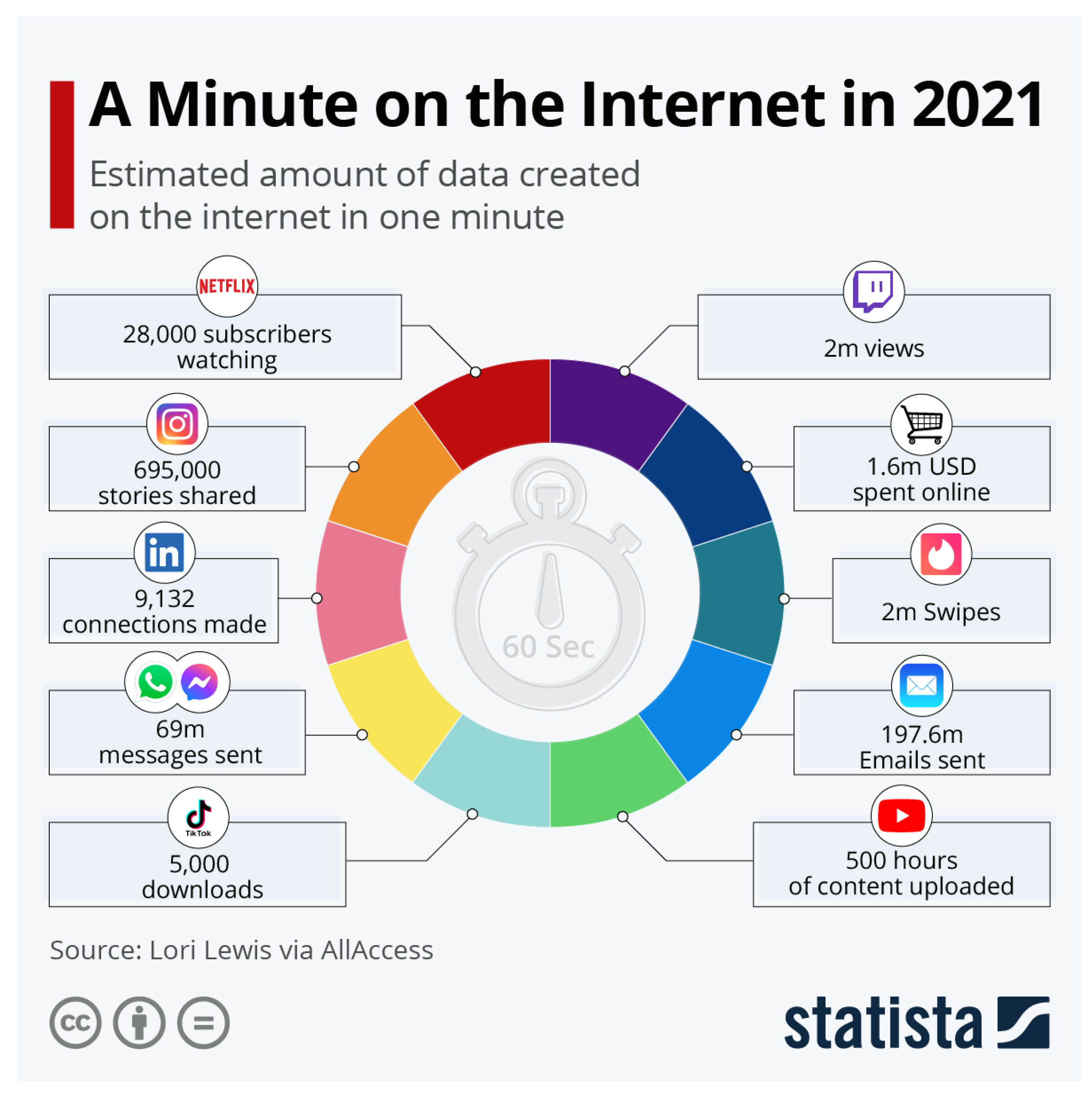
Whether in social networks, media, or medicine, many industries collect and process a growing volume of multimedia content objects (i.e., representations of real-world scenes, such as videos, images, textual descriptions, audio recordings, or combined objects). Statista [1] describes an increase in the volume of photos taken with a smartphone, from 660 billion in 2013 to 1.2 trillion in 2017. When comparing the volume of titles on video streaming services from fall 2021 [2] and summer 2022 [3], annual growth can be observed. Research data sets grow with similar rates, as the National Library of Medicine shows. Founded as Open-i in 2012 with 600,000 [4] assets, the collection grew to 1.2 million in 2022 [5]. Similar rates are shown in Figure 1; in one minute on the Internet [6], 695,000 Instagram [7] stories are shared, 500 hours of YouTube [8] content is uploaded, and 197 million emails are sent.
Mechanisms for the efficient indexing and fast retrieval of these multimedia content objects are essential to manage this large volume of information. Cloud computing [9] and big data technologies [10] enable the storage and processing of these amounts of multimedia content objects. Recent improvements in machine [11] learning, such as deep learning [12], enabled the automated extraction of features from the raw multimedia content object by employing object recognition [13], face identification, and further methods. The increasingly high resolution in multimedia content objects, such as 32-bit audio recording, 8K video recording, and 200-megapixel smartphone cameras, allows the extraction of features with a high level of detail (LOD) from the content of multimedia content objects. All this extracted feature information can be efficiently organized and indexed by graph-based technologies. In previous work [14], we introduced the Multimedia Feature Graphs (MMFG), Graph Codes (GCs), and Graph Code algorithms. Evaluations showed that they are fast and effective technologies for Multimedia Information Retrieval (MMIR) [15] and that Graph Codes can perform better as graph databases. According to [16], the acceptable response time for users is around one second. However, information retrieval in large multimedia collections and a high LOD still result in processing times above the margin of one second. Previous experiments show a potential speedup of the execution times of the Graph Code algorithm through the parallelization of Graph Code algorithms. One of the remaining research questions is how to efficiently parallelize Graph Code algorithms and whether this can lead to a speedup.
To answer this question, in this paper, we introduce several approaches to scale Graph Code algorithms. The scaling approaches explore horizontal and vertical scaling. While vertical scaling aims to employ massively parallel processing hardware, such as Graphic Processing Units (GPUs) [17], horizontal scaling aims at distributed computing systems, such as Apache Hadoop [18]. Section 2 summarizes the current state of the art and related work. Section 3 discusses the mathematical and algorithmic details of parallel Graph Code algorithms and their transfer to parallel systems. The models presented show significant potential to speed up Graph Code processing on GPUs. These models have been used for the proof-of-concept implementation given in Section 4. Finally, the evaluation in Section 5 shows the detailed results of the experiments on its efficiency. Section 6 concludes and discusses future work.
2. State of the Art and Related Work
This section offers a synopsis of current techniques and standards in the field of Multimedia Information Retrieval, as well as a summary of related research. Initially, a foundation is established on existing approaches, followed by the introduction of the Graph Code [14] concepts, an efficient and performant indexing technique. The scaling approaches are based on parallelization technologies and, hence, a brief overview of applicable parallelization options is given. Finally, in this section, the starting points for scaling Graph Code processing are summarized.
2.1. Information Retrieval
Information retrieval [19] aims to find information in large information collections. Multimedia Information Retrieval particularly targets collections with image, video, text, or audio assets (i.e., multimedia content objects). MMIR systems are designed to support these use cases. To search for information, the main component is a search engine. The search engine has an information database containing the list of multimedia assets in the collection and also an index of them. The index contains metadata about the assets. Semantic metadata connect the features and make them machine processable. Metadata can be supplied or generated by feature extraction. In order to organize features, graph-based methodologies and structures are frequently employed, given that feature information relies on information nodes and the connections that exist between these nodes [20]. The increasing number of features requires a mechanism to structure features, detect inconsistencies, and calculate the relevance of each feature, which we describe next.
2.2. Multimedia Features and Multimedia Feature Graphs
The Multimedia Feature Graph (MMFG) [21] is a weighted and directed graph [22], whose nodes and edges represent features of multimedia assets. The Generic Multimedia Annotation Framework (GMAF) [23] is an MMIR system for multimedia assets that uses MMFGs as an index and access method. GMAF provides a flexible plugin architecture that allows the processing of various multimedia asset types to extract features that are stored as metadata in the MMFG. The extracted features are contributed to the MMFG, which can be further processed. Extensions of MMFGs have led to semantic analysis, such as Semantic Multimedia Feature Graphs (SMMFGs) and Explainable SMMFGs (ESMMFGs) [24]. Despite these extensions, the graph-based structure of MMFGs remains and can lead to slow processing times. When the LOD of the assets increases, the number of elements in the MMFG also increases, which further increases the processing times. To address this, Graph Codes were introduced for faster indexing [14]. Therefore, it is important to experiment with an improved processing model to reduce processing times. This is outlined in the next subsection.
2.3. Graph Codes and Algorithms
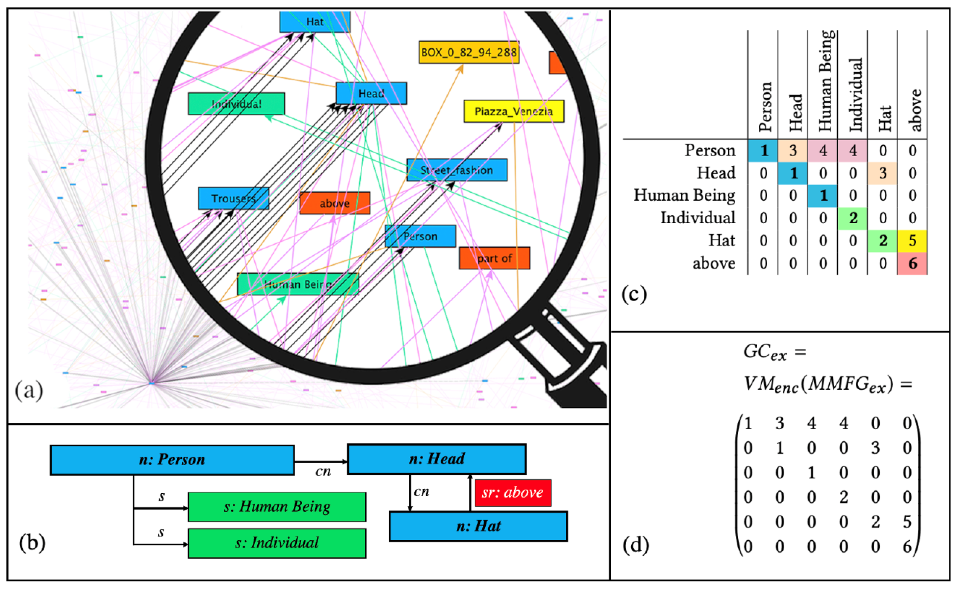
Graph Codes [14,25] are a 2D transformation of a multimedia feature graph that is encoded using adjacency matrix operations [26]. GCs have been shown to be more efficient for similarity and recommendation searches than graph-traversal-based algorithms. Graph Codes represent the labels of feature graph nodes and edges in the form of vocabulary terms. Based on the adjacency matrix of such a feature graph, these are used as row and column indices. The elements of the matrix represent the relationships between the vocabulary terms. The type of the edge in the graph is encoded as the value of the matrix element. Figure 2 illustrates a simple example of a multimedia feature graph (see Figure 2a), a detailed section from the graph (Figure 2b), its corresponding GC in a table representation (Figure 2c), and the GC matrix (Figure 2d).
GCs contain a dictionary of feature vocabulary terms () and represent the relationships between these terms using the matrix field . A similarity metric triple has been defined for GCs. The feature metric is based on the vocabulary, the feature relationship metric is based on the possible relationships, and the feature relationship type metric is based on the actual relationship types.
Semantic Graph Codes (SGCs) [23] are an extension of GCs that incorporate additional semantic structures using annotation with semantic systems such as RDF, RDFS, ontologies, or Knowledge Organization Systems [28,29,30]. This additional semantic information can help to bridge the semantic gap between the technical representations of multimedia feature graphs and their human-understandable meanings.
With the introduction of semantics to the MMFGs in [24], we introduced additional metrics to improve the efficiency and effectiveness of Graph Codes for MMIR. First, the feature discrimination is defined as the difference in the number of nonzero Graph Code fields for two feature vocabulary terms of a given Graph Code or Semantic Graph Code. TFIDF [31] is a numerical statistic used in natural language processing to evaluate the importance of a word in a document. An adapted TFIDF measure for Graph Codes can use to reveal how representative a term is for a single document—in this case, an SGC. The Semantic Graph Code collection corresponds to the TFIDF documents. With , it can be used to define a threshold for a collection to exclude less relevant features from the retrieval process. Alternatively, can be used to weight terms according to the use case. This requires the pre-processing of the Graph Codes by removing the non-relevant vocabulary terms. This step needs to be performed when the relevance threshold is changed, or whenever a multimedia content object is added to or removed from the collection.
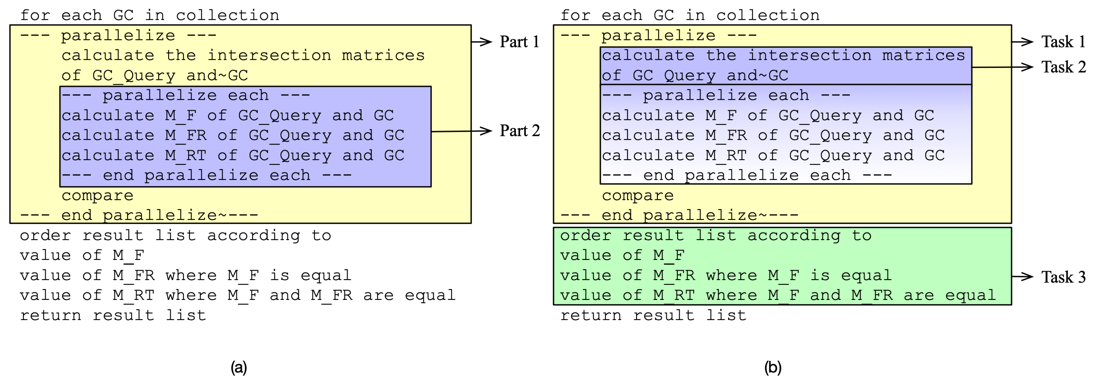
Introduced in [14], the basic algorithm for the comparison and order of Graph Codes in a collection is listed in pseudocode below.
for each GC in collection
--- parallelize ---
calculate the intersection matrices
of GC_Query and~GC
--- parallelize each ---
calculate M_F of GC_Query and GC
calculate M_FR of GC_Query and GC
calculate M_RT of GC_Query and GC
--- end parallelize each ---
compare
--- end parallelize~---
order result list according to
value of M_F
value of M_FR where M_F is equal
value of M_RT where M_F and M_FR are equal
return result list
Experiments with a proof-of-concept (POC) implementation of the algorithm showed that parallel instances can process individual parts of a Graph Code collection in less time on multicore CPUs compared to a single instance. Compared to a single instance with an execution time of 635 s, 16 instances could process the same volume of data in 65 s [32]. Therefore, we explored approaches for the parallel processing of Graph Codes.
2.4. Parallel Computing
The scaling of algorithm processing can either be achieved by higher-performance computing resources or by executing parts of the algorithm in parallel. Higher performance is usually an upgrade of hardware, which is called vertical scaling. Parallel computing can be achieved in many ways. In a single computer, multiple processing units can exist in the form of multicore Central Processing Units (CPUs) [33] or coprocessors such as Graphics Processing Units (GPUs) [17] or Field-Programmable Gate Arrays (FPGAs) [34]. While multicore CPUs work in Multi-Instructions Multiple Data (MIMD) [35] fashion, GPUs usually work in a Single-Instruction Multiple Data (SIMD) [35] method. Although MIMD is suitable for general purpose computing, it is limited for massive parallelization [36] (p. 181). SIMD is optimal for massive parallelization, but only in cases where the same instructions are being applied to the data. Both concepts can be found in modern processors, e.g., Apple M-series [37] and A-series [38], Nvidia G200 [36] (p. xii), CPU AVX extension [39]. Additionally, systems can contain multiple processing units, such as multi GPUs. State-of-the-art approaches [40,41,42] mainly apply GPUs for performance improvements.
Another option for in-system parallelization is distributed computing. Instead of spreading the operations on the data to different processing units in the system, the data and the instructions are distributed to many systems. This is called horizontal scaling. Many frameworks are available to support coordination in distributed computing. Frameworks such as Hadoop [18] or TensorFlow [43] can be used to coordinate parallel execution on large clusters of computers.
On a high level, a task to parallelize can be classified as Task-Level Parallelization (TLP) [33] or Data-Level Parallelization (DLP) [33]. While tasks in TLP can be general purpose and very different from each other, in DLP, the same operation is applied to different data, similar to a matrix multiplication. Given Flynn’s taxonomy [35], for the parallel computation of multiple data, SIMD or MIMD processors can be used. TLP works well with MIMD processors, while, for DLP, SIMD processors are more suitable. As mentioned above, modern processors cannot simply be categorized as SIMD or MIMD, because they often have features of both categories. Multi-Core CPUs such as an Intel i9 [39] work as MIMD but have SIMD extensions such as AVX. GPUs operate as SIMD, but Nvidia CUDA [44] GPUs can also operate as MIMD. Hence, a detailed analysis is needed to find the most suitable processor for a certain task.
To take advantage of the potential for parallel computing, applications and algorithms need to be modified. The method of algorithm decomposition [45] (p. 95) can be applied to identify sections that can run in parallel. Recursive decomposition searches for options for a divide-and-conquer approach. Data decomposition looks for parts of the algorithm that apply the same operation to parts of the data to be processed. Further techniques exist, and they can be applied in hybrid. The result of the algorithm decomposition is a Task Dependency Graph (TDG). A TDG is a directed acyclic graph that signifies the execution process of a task-oriented application. In this graph, the algorithm’s tasks are depicted as nodes, while edges symbolize the interdependencies among tasks. This relationship denotes that a task can only commence its execution once its preceding tasks, represented by incoming edges, have been successfully completed. The TDG can be used to organize an algorithm for the targeted system.
According to [46], the efficiency gain of parallel executions is defined as the speedup S, which is the ratio of the sequential execution time and the execution time on n processors :
Amdahl’s [47] and Gustafson’s [48] laws can be used to calculate the theoretical speedup, based on the fractions of the program, which can be parallelized or not, and the number of execution units. While a detailed discussion of the speedup of our modeled algorithms follows in Section 3.4, the previously given pseudocode can be used as a first approximation: the not parallelizable part of the program s is the order result list, which is around 10% of the program, so the parallelizable part p is 90%. According to Gustafson’s law, the speedup S on 10 cores N would be .
However, the following decomposition of the algorithm to calculate and order the Graph Code metrics will produce a TDG. The characteristics of the tasks can indicate which execution model provides the best acceleration yields.
2.5. Discussion and Open Challenges
Summarizing this body of scientific research, Graph Codes have shown promising performance compared to graph traversal operations. Although Graph Codes are faster than comparable methods, processing large multimedia collections and a high LOD result in optimizable processing times. Previous experiments with the algorithm show options for efficiency gains by parallelization, but the full application of parallelization remains an open challenge. This includes the creation of models for parallel Graph Code algorithms, the transfer to available technology, and the evaluation of the corresponding algorithms and models. To parallelize Graph Code processing, various options are available. For vertical scaling, GPUs are an option, but a detailed analysis is necessary. The decomposition techniques can be applied to characterize the tasks of the algorithm. The resulting TDG indicates which hardware fits best for the parallelization of the algorithm.
3. Modeling and Design
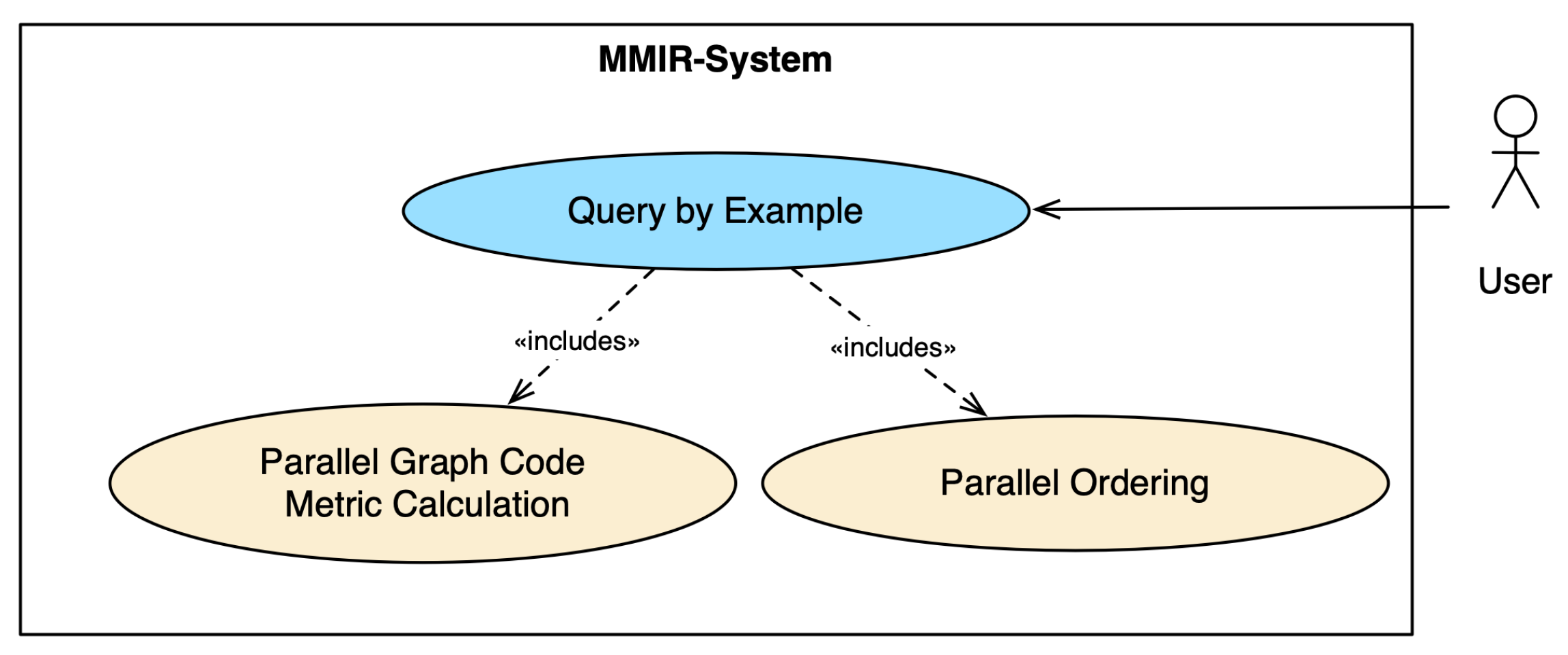
For our modeling work, we employed the User-Centered System Design [49] by Norman and Draper and the Unified Modeling Language (UML) [50]. The central use case for our modeling work is similarity search, as shown in Figure 3. The objective of similarity search is to discover objects that bear a resemblance to a designated query object, adhering to a specific similarity criterion provided. With the user in focus, we aimed for an optimized user experience in terms of reducing runtimes for the implementation of the use case. In the case of MMFGs and Graph Codes, in the first use case, Parallel Graph Code Metric Calculation, the calculation of the metrics’ values for the query Graph Code and all Graph Codes in the collection is happening. In the use case Parallel Ordering, the list of items and metrics is ordered by the highest similarity by comparing the metric values. Parallel algorithms are explored for both steps.
In the following sections, we employ the described decomposition techniques for the Graph Code algorithms and model different parallel approaches. The modeled approaches are examined for their theoretical speedup and applicability to parallelization technologies.
3.1. Parallel Graph Code Algorithms
The similarity search based on Graph Codes calculates the metric values for each Graph Code in the collection against the query Graph Code and orders the results. The pseudocode of Section 2.3 describes the algorithm. We applied the decomposition techniques (Section 2.4) to the algorithm and modeled a Task Dependency Graph (TDG).
Starting with the first step, the iteration over all items n in the Graph Code collection can be decomposed by the divide-and-conquer method. As the individual metric calculations do not have dependencies, they can be split into n parallel steps. Next, the calculation of intersection matrices and metric calculation contain comparison of the elements in both matrices. Hence, the data decomposition can be used, and each comparison step can be done in parallel. In a consecutive step, the individual comparison results are used to calculate the Graph Code metric values. The calculation of the three metric values could also be parallelized, but compared to the rest of the algorithm, the number of instructions is low and, therefore, the potential is also low. Finally, the ordering of the results can be parallelized.
In summary, the decomposition identified three tasks:
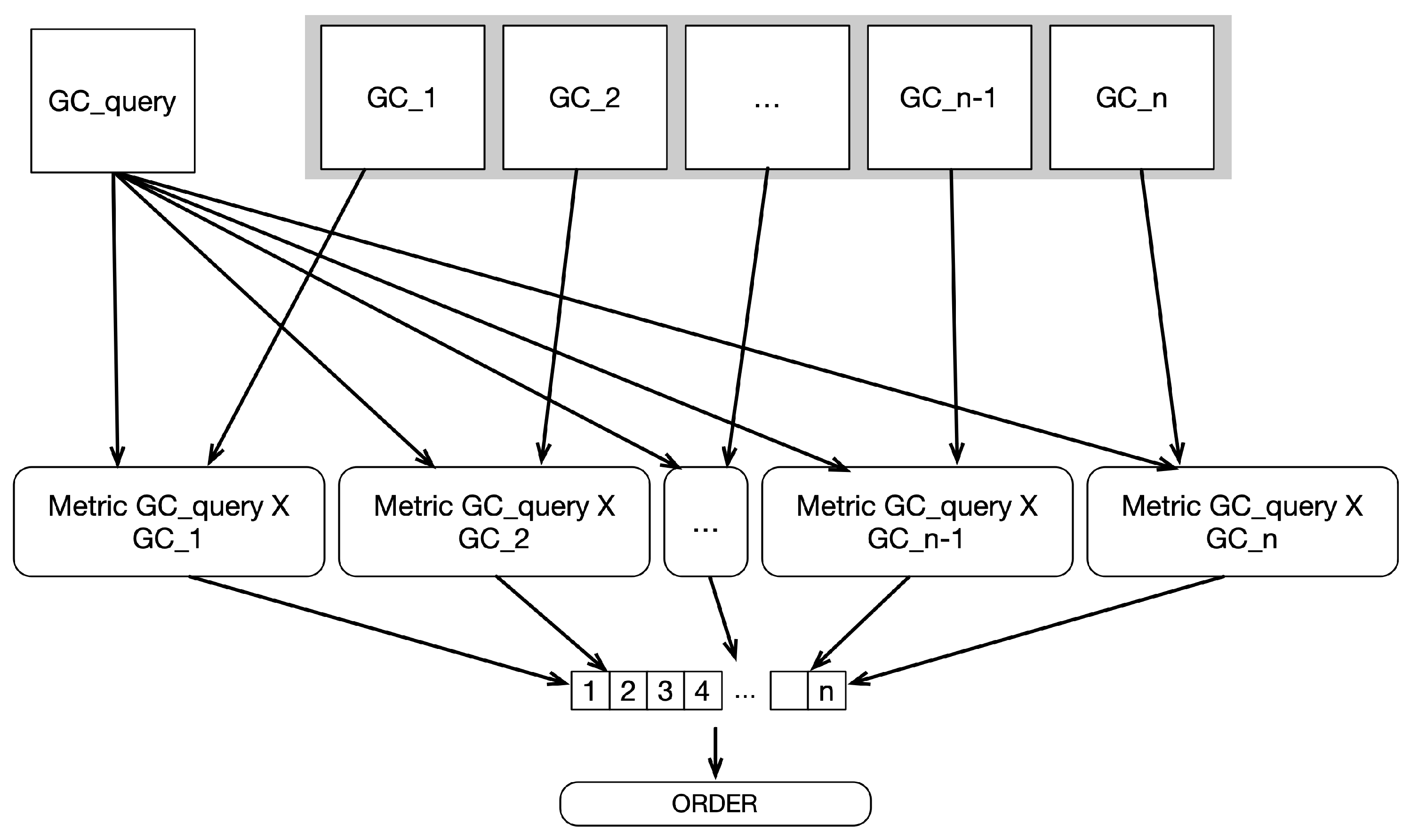
- Task 1: Calculate the metrics for each pair of Graph Codes (see Figure 4). The metric calculation itself can be decomposed by the data decomposition method.
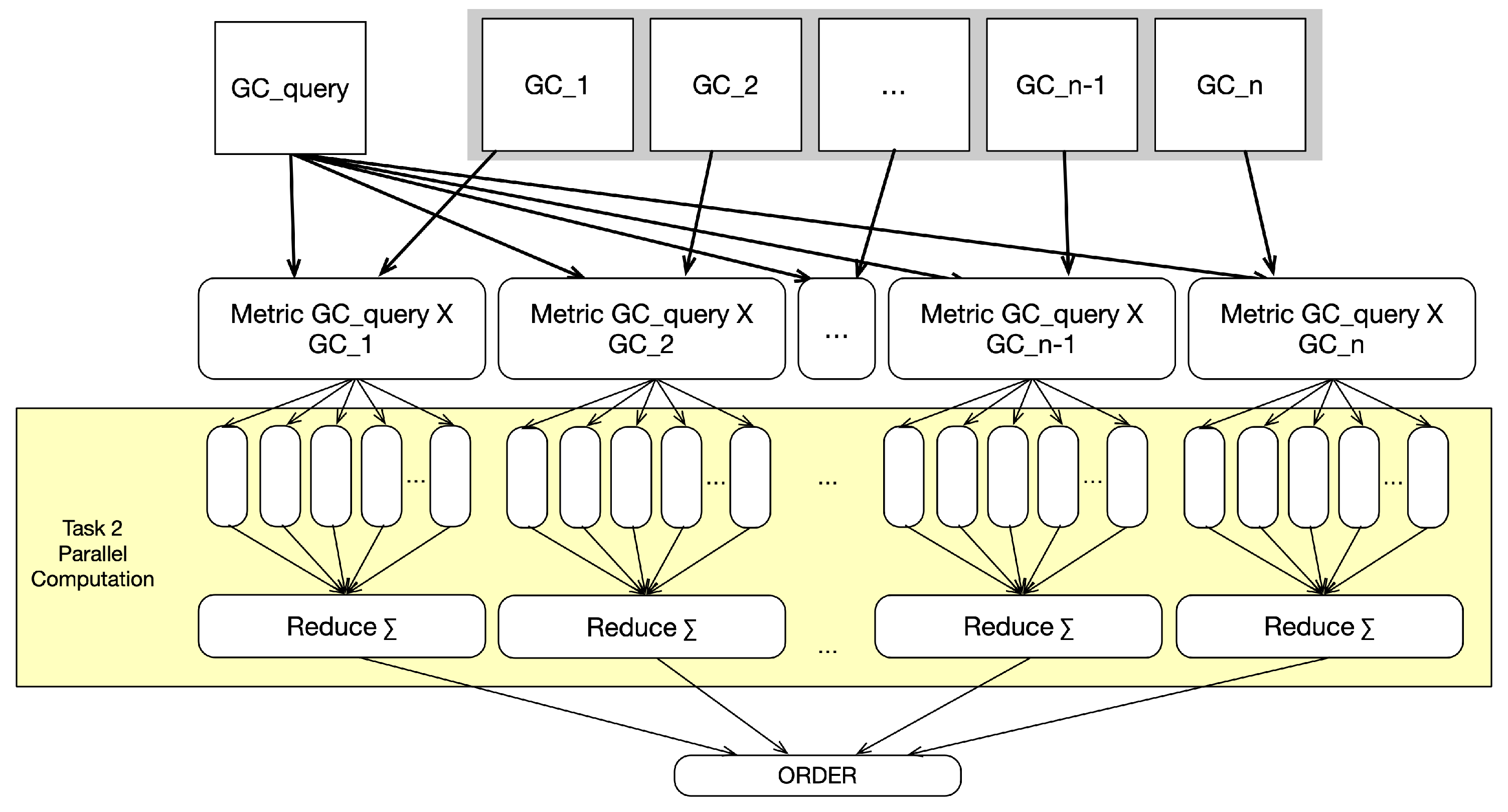
- Task 2: For each element in the dictionary and the matrix of , find the matching elements in and calculate the values according to the metrics (see Figure 5).
- Task 3: After the metrics are calculated, the result set should be ordered.
Compared to the parallelization points indicated in the pseudocode, the identified tasks are different, as shown in Figure 6, where the initial version shows two parallel parts (Figure 6a), and the new version shows the three decomposed tasks (Figure 6b). Task 1 and Task 2 are part of the sub-use case Parallel Graph Code Metric calculation of the use case similarity search. Task 3 maps to the use case Parallel Ordering of the use case similarity search.
The identified tasks can, but do not need to, run in parallel, regardless of whether the other tasks are sequential or parallel. Hence, different versions can be modeled. The remainder of this section discusses different models.
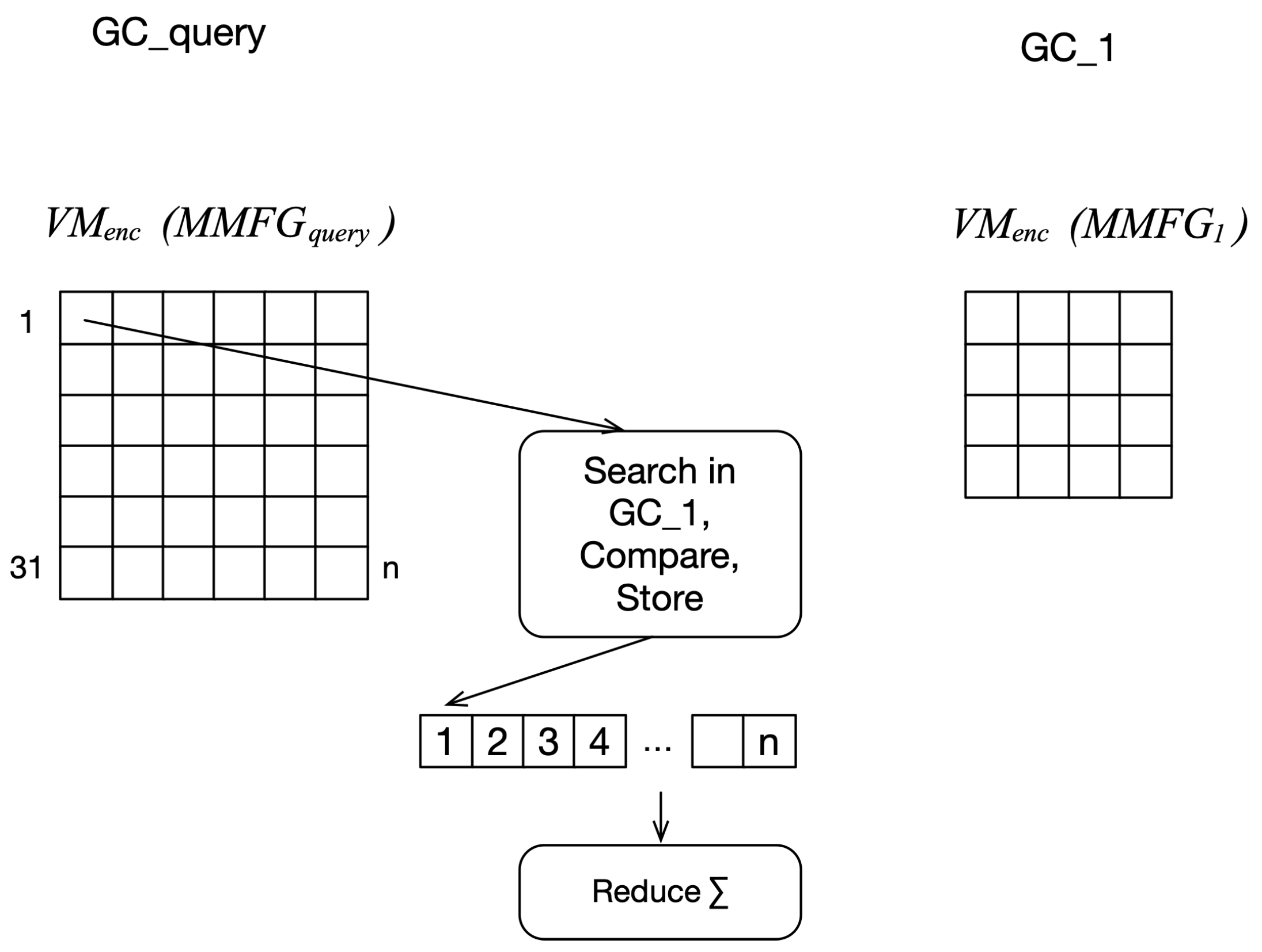
Task 1, the iteration over the collection, is an obvious task to run in parallel and has no interdependencies between each calculation of the metric, as shown in the TDG in Figure 4. A metric calculation uses two Graph Codes as input. For a similarity search, one of the inputs is the reference Graph Code , and the other is an element from the collection . Each of these calculations can be executed independently and thus arbitrarily in parallel. The calculated metric values will be stored in a result array; the position is correlated with the position in the collection. The parallelization can be done on thread-level parallelization and, therefore, run on multicore CPUs and GPUs, as well as with distributed processing. Listing 1 shows the start and end of the parallelization for Task 1 parallelization.
| Listing 1. Pseudocode of Task 1 parallelization. |
| 1 --- START TASK 1 -> TLP parallelise --- |
| 2 for each GC in collection |
| 3 --- calculate the intersection of GC_Query and~GC --- |
| 4 for each element in GC_Q->VM |
| 5 Check Intersection with GC_Q |
| 6 Calculate M_F, M_FR, M_RT from m_res array values |
| 7 --- END Task 1 TLP parallelize --- |
| 8 order result list according to |
| 9 value of M_F |
| 10 value of M_FR where M_F is equal |
| 11 value of M_RT where M_F and M_FR are equal |
| 12 return result list |
For Task 2, finding intersections in the two matrices can be processed in parallel, but the findings, as well as the check for the feature relationship metric and feature relationship type metric, need to be stored in intermediate storage, as shown in Figure 5. This part of Task 2 is named Task 2a. As a subsequent step, the storage is summed up and the values are used for the calculation of the final metric values. This step is Task 2b. For large matrices in the millions, due to the high LOD, summing up the values can be done in parallel with reduction approaches [51]. Listing 2 shows the start and end of the parallelization in the case of Task 2.
| Listing 2. Pseudocode of Task 2 parallelization. |
| 1 for each GC in collection |
| 2 --- calculate the intersection of GC_Query and~GC --- |
| 3 --- START TASK 2a -> SIMD parallelize --- |
| 4 for each element in GC_Q->VM |
| 5 Check Intersection with GC_Q, store in m_res array |
| 6 ... |
| 7 --- END TASK 2a SIMD parallelize --- |
| 8 --- START TASK 2b -> TLP parallelize |
| 9 reduce m_res arrays |
| 10 --- END TASK 2b TLP parallelize --- |
| 11 Calculate M_F, M_FR, M_RT from m_res array values |
| 12 order result list according to |
| 13 value of M_F |
| 14 value of M_FR where M_F is equal |
| 15 value of M_RT where M_F and M_FR are equal |
| 16 return result list |
The final Task 3, the ordering of the metrics, has a dependency on all preceding tasks because it needs all the calculated metrics as input. The task itself can be done with parallel versions of QuickSort [52] or RadixSort [53].
Task 1 can run in parallel with a sequential metric calculation, or in parallel, as described with Task 2, as shown in Figure 7. Executing Task 1 in sequence and only running Task 2 in parallel is also possible, as shown before in Figure 5. The following Listing 3 shows the start and end of the tasks and the type of parallelization for all the tasks.
| Listing 3. Pseudocode of Task 1, 2, and 3 parallelization. |
| 1 --- START TASK 1 -> TLP parallelise --- |
| 2 for each GC in collection |
| 3 --- calculate the intersection of GC_Query and~GC --- |
| 4 --- START TASK 2a -> SIMD parallelize --- |
| 5 for each element in GC_Q->VM |
| 6 Check Intersection with GC_Q, store in m_res array |
| 7 ... |
| 8 --- END TASK 2a SIMD parallelize --- |
| 9 --- START TASK 2b -> TLP parallelize |
| 10 reduce m_res arrays |
| 11 --- END TASK 2b TLP parallelize --- |
| 12 Calculate M_F, M_FR, M_RT from m_res array values |
| 13 --- END Task 1 TLP parallelize --- |
| 14 --- START TASK 3 -> TLP parallelize --- |
| 15 order result list according to |
| 16 value of M_F |
| 17 value of M_FR where M_F is equal |
| 18 value of M_RT where M_F and M_FR are equal |
| 19 --- END TASK 3 TLP parallelize --- |
| 20 return result list |
Overall, the initial algorithm can be broken down into three tasks, and each task can be parallelized or in sequence. In the next section, we define algorithms from the different combinations.
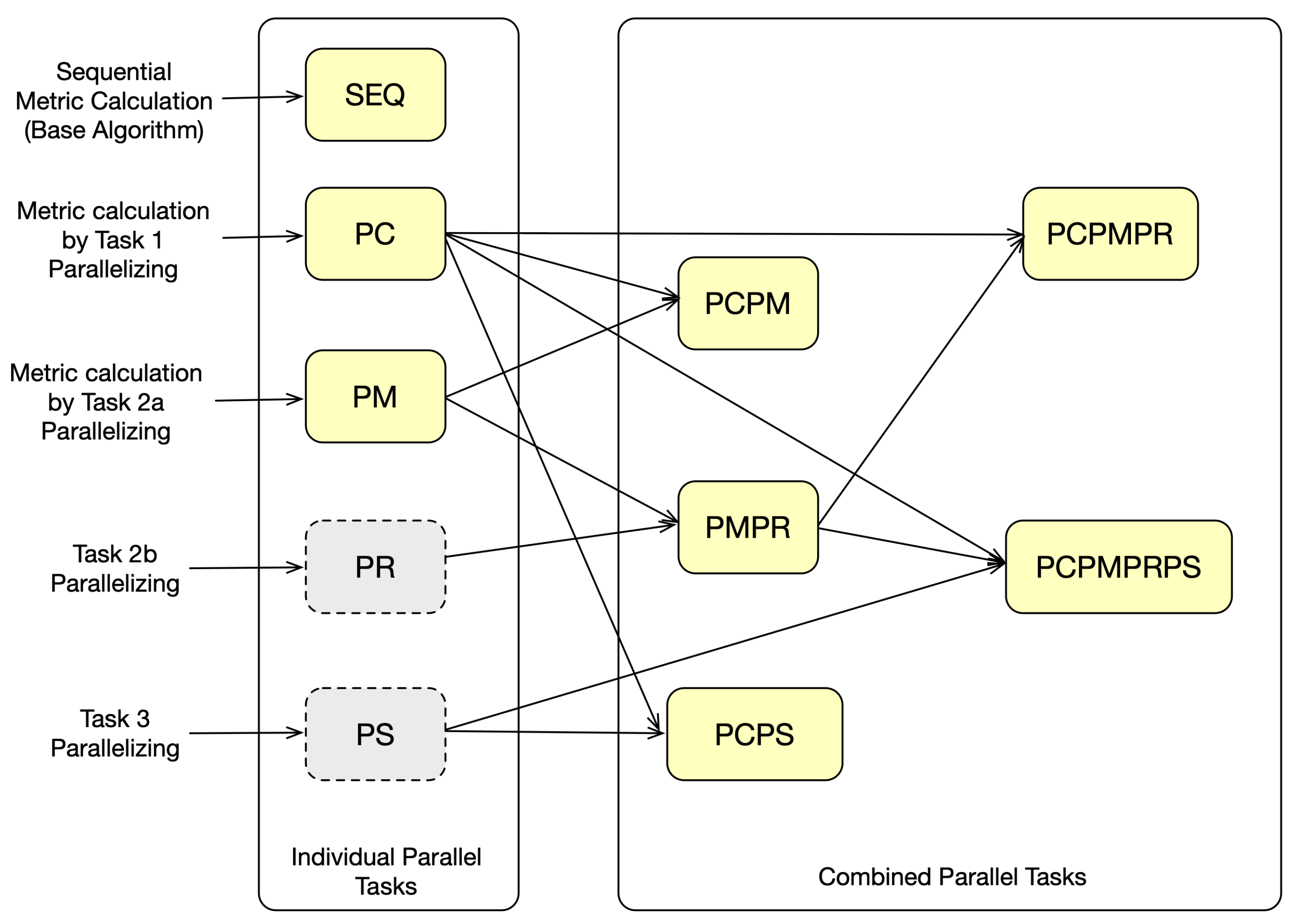
3.2. Definitions
Similarity search can be processed through the three consecutive tasks, each of which can be parallelized or sequential. Hence, the different combinations result in several algorithms, which are defined as follows:
- For reference, we define the sequential algorithm without parallel steps as Sequential ().
- We define the (thread-level) parallelization of Task 1 only as Parallel GC Compute ().
- The parallel computation of Graph Code metrics, as described as Task 2a, is defined as Parallel Metric Sequential Reduce ().
- The combination of Tasks 2a and 2b is defined as Parallel Metric Parallel Reduce ().
- For very large Graph Codes, it may be useful to use alone, but it can be combined with , which we define as Parallel GC Compute with Parallel Metric ().
- Accordingly, in combination with is defined as Parallel GC Compare with Parallel Metric Parallel Reduce ().
- Finally, if parallel sorting is also applied, we define the combination with as Parallel Compute and Parallel Sort ().
- Consequently, with and Parallel Compute Parallel Metric Parallel Reduce Parallel Sort is defined as ().
- If parallel sorting is also applied, we define the combination with as Parallel Compute and Parallel Sort ().
- Respectively, all parallelized tasks are defined as Parallel Compute Parallel Metric Parallel Reduce Parallel Sort ().
Figure 8 illustrates the possible combinations and the resulting algorithms. The individual Tasks 2b and 3 alone are not useful; therefore, they are colored in gray.
Based on the described models of parallel Graph Code algorithms, we will discuss the transfer to modern processors and show the potential speedup.
3.3. Potential Parallelization on Modern Processors
Modern processors are designed as multicore processors. They can execute instructions in parallel, but the execution model differs. While MIMD processors have an individual instruction counter for each core, SIMD processors share an instruction counter. A shared instruction counter means that every core executes all statements for all paths of input data. If a branch of the code (e.g., if statement) is not executed in one parallel path, the core omits the instruction step and cannot execute other instructions. This effect is called thread divergence. The branching characteristics of parallel tasks impact the utilization of a SIMD processor and, hence, the efficiency of the algorithm. However, SIMD processor designs can have many more cores and can achieve massive parallelization.
The characteristics of the modeled parallel Graph Code algorithms are both advantageous and disadvantageous for parallelization. The individual tasks have a low degree of dependency and show a gather pattern, which means that inputs can be grouped and processed individually, and each output can be stored in an individual place. This indicates the applicability for SIMD. On the other hand, the calculation of metrics implies the creation of intersections of two Graph Codes. The number of intersections depends on the size and similarity of the Graph Code. This indicates that thread divergence is likely.
The algorithm can be parallelized at thread level, which means that every calculation can be put into a thread and executed in parallel. This is suitable for both types of processors: multicore CPUs (MIMD) and modern GPUs (SIMD). As Task 2 algorithms constitute data-level parallelization, it loads the data once and processes each item. Data-level parallelization is more suitable for GPUs, but in the case of heterogeneous Graph Codes, thread divergence can limit the effectiveness. However, the low degree of dependency allows for processing many calculations in parallel, employing all available cores. Given a processor with 16,000 cores, such as the Nvida H100 [54], 16,000 Graph Code metric calculations can be performed in parallel.
To reduce or even eliminate the possible performance impact of thread divergence, the Graph Codes can be grouped by size. Executing same-size groups could reduce thread divergence. This method has been used in similar cases [55]. Another approach is to employ the previously described Feature Relevance [24]. Graph Codes with only relevant features should increase the performance with a minimal loss of accuracy. The impact on parallel Graph Code algorithms works as follows.
Depending on the vocabulary width (LOD) used in the MMFGs, the resulting Graph Codes can be sparse or dense. With a high LOD, Graph Codes tend to be large and sparse. For the calculation, this leads to many unnecessary comparisons to obtain the intersections of two Graph Codes. For a similarity search, it is questionable to have many terms used in only one Graph Code or in every Graph Code. By applying techniques such as TFIDF, the density of the information in the resulting SMMFGs and the semantic Graph Codes increases. The resulting semantic Graph Codes have similar dimensions and a similar number of intersections. Both may be beneficial to the effect of thread divergence and, hence, to the efficiency of parallel Graph Code algorithms.
A further approach for Task 2a could replace the search of corresponding feature vocabulary terms in the Graph Code to compare with a lookup table, such as an inverted list [56]. This approach could be applied to the sequential and parallel versions of the algorithms.
A benefit of the modeled algorithms is that no more pre-processing is needed than producing the Graph Codes. The approaches Semantic Graph Codes and inverted lists require further pre-processing.
In summary, the characteristics of the parallel algorithm show high potential for acceleration. In the next section, we deduce the theoretical speedup.
3.4. Theoretical Speedup
The performance of parallel Graph Code algorithms can be compared with the sequential version. The improvement is measured as speedup S, which is the ratio of parallel to sequential runtime, where p is the number of processors around a problem of size n. is the execution time of the best serial implementation and is the parallel implementation. In this subsection, we will focus on the algorithm .
The calculation of the metric values is performed on a collection of Graph Codes . This corresponds to
The value n corresponds to the number of Graph Codes in a collection
Each Graph Code has a variable word list with a length l corresponding to the dimension of the Graph Code value matrix .
Regarding the sequential metric computation of two Graph Codes and , the runtime can be mainly described by the sizes l of the respective Graph Codes with the following factors. For each element in the matrix of Graph Code , the corresponding values of Graph Code must be searched and compared. as the number of elements in the word list of the query vector and corresponding is the length of the word list in the vector to compare .
When calculating the metrics of a collection of Graph Codes , the calculation is performed for Graph Code against each element in the collection. Hence, the calculation happens n times, the number of Graph Codes in the collection. Since the GCs vary in length, the individual runtimes are summed up.
In consideration of the parallel algorithm, can now be divided by the number of execution units (CPU cores or CUDA cores) c. This results in
By parallelizing the steps for each element of the Graph Code matrix , this can be divided among the number of execution units c. To form the sum, the buffer size l must be calculated.
Looking at current top-end GPUs such as the Nvidia H100 with 16,896 cores,
As measured in previously published experiments (source), the calculation of 720,000 Graph Codes took 635 s in an instance using a single thread. Hence, employing the parallel algorithms could lead to a reduction in the processing time down to 0.038 s or a theoretical speedup of 16.711.
Graph Codes and the modeled algorithms show high potential for massive parallel processing. Next, we summarize the section and discuss the implementation and evaluation of the algorithms.
3.5. Discussion
In this section, we present the conceptual details of parallel Graph Code algorithms, their mathematical background and formalization, and the conceptual transfer of parallel algorithms to processors. The application of the decomposition methods showed that the Graph Code metric calculation is massively parallelizable. In theory, the only limiting factor is the number of available cores and memory.
The algorithm variants show huge speedup potential on different multicore processor systems. Considering an implementation for SIMD GPUs with a shared instruction counter, the heterogeneity of Graph Codes in a collection could lead to the inefficient utilization of GPU resources. We presented the options of grouping Graph Codes by size or homogenization with TFIDF. As it is a theoretical examination, an implementation of the parallel algorithm and an evaluation of the efficiency is needed.
With regard to distributed computing, the algorithm could be used because Tasks 1 and 2 are without dependencies. If the collection is distributed, all nodes can calculate their portions; only the final Task 3 (ordering) needs to be computed on one node with all intermediate results. Implementing and evaluating this remains an open challenge.
For an evaluation of real performance, we decided to implement some variants of the algorithms. To compare speedups on CPU and GPU, we decided to implement for Threads and CUDA. In the case of a very high LOD, algorithms and could be beneficial. To test their efficiency, they were implemented in CUDA. For a comparison of ordering the result list (Task 3) on the GPU and CPU, was implemented for CUDA. Our implementation is discussed in Section 4 and the evaluation results given in Section 5.
4. Implementation and Testing
To test the different algorithms, we implemented a proof-of-concept (PoC) application to measure and compare execution times. The application flow follows the use case Query by Example; thus, the processing times are similar to what a user would experience in a real application. We used different hardware systems and software libraries. The algorithm modeling showed high potential for parallel execution. Hence, we wanted to run the algorithms on multicore CPUs and GPUs. For the multicore CPUs, we used the POSIX-Threads library, and for GPUs, we selected the CUDA platform because it is used in comparable research. The application and the algorithms were implemented in C/C++, which allows portability and a reduced possible execution overhead of any interpreters or intermediate frameworks. The application reads the Graph Code data initially from files and stores it in the main memory. In case of CUDA, the data were transformed into a simple data structure and transferred from the main memory to the GPU memory before the calculation, and therefore before measuring the runtimes of the algorithms.
Different versions of the algorithms were implemented. An overarching comparison between sequential, CPU parallel, and GPU parallel runtimes can be made with the algorithm Parallel GC Compute . We implemented the algorithm in a sequential version, ; a CPU POSIX-Threads version, ; and a CUDA parallel version, . For the CPU parallel algorithm, the number of utilized cores can be set. The CUDA implementation is optimized for maximum GPU utilization. For for CUDA, each Graph Code similarity metric calculation is packaged in a parallel executable unit, a kernel. Listing 4 shows parts of the kernel as a function declaration in lines 1–35. The listing demonstrates the process flow for a number of Graph Codes (numberOfGCs), stored at the pointer gcMatrixData (line 2) and gcDictData (line 2), accessible by helper arrays gcMatrixOffsets, gcMatrixSizes, and gcDictOffsets (lines 3–4). First, the index of the Graph Code in the collection is located with the CUDA thread model (line 6). Next, the values gcQuery (line 4) and index, both containing the positions of the two Graph Codes to compare, are used to access the data points in the corresponding arrays—for example, in line 11 or line 14. The lines 19–34 show the metric calculation and the storage of the values in the metrics array. The metrics array will be transferred from the GPU memory to the main memory after execution, demonstrated in the function demoCalculateGCsOnCuda (lines 37–70), with the transfer in lines 65–67. This example also shows that most of the actual calculation is done in the CUDA kernel and, hence, in a parallel way. The sequential part of the algorithm is low, which is in line with the previously mentioned application of Gustafson’s law and the theoretical speedup calculation.
For the sorting, we used sequential sorting and adapted CUDA-QuickSort [52] to compare the metric values.
For the CUDA implementation, thread divergence can have a negative impact on execution times, and because of the heterogeneity of Graph Codes, it is likely to happen. To compare the differences, the application either loads a real dataset or generates an artificial Graph Code.
| Listing 4. Partial code of the Parallel Graph Code metric calculation according to PC. |
| 1 /∗ metric calculation ∗/ |
| 2 __global__ void cudaGcCompute(unsigned short ∗gcMatrixData, unsigned int ∗gcDictData, |
| 3 unsigned int ∗gcMatrixOffsets, unsigned int ∗gcMatrixSizes, |
| 4 unsigned int ∗gcDictOffsets, int gcQuery, int numberOfGcs, Metrics ∗metrics) { |
| 5 |
| 6 unsigned int index = threadIdx.x + blockIdx.x ∗ blockDim.x; |
| 7 if (index >= numberOfGcs) |
| 8 return; |
| 9 |
| 10 int sim = 0; |
| 11 int elementsGc1 = sqrtf((float) gcMatrixSizes[gcQuery]); |
| 12 int elementsGc2 = sqrtf((float) gcMatrixSizes[index]); |
| 13 |
| 14 unsigned int off1 = gcDictOffsets[gcQuery]; |
| 15 unsigned int off2 = gcDictOffsets[index]; |
| 16 |
| 17 ... // Metric Calculation |
| 18 |
| 19 metrics[index].similarity = 0.0; |
| 20 metrics[index].recommendation = 0.0; |
| 21 metrics[index].inferencing = 0.0; |
| 22 metrics[index].similarity = (float) sim / (float) elementsGc1; |
| 23 metrics[index].idx = index; |
| 24 if (num_of_non_zero_edges > 0) { |
| 25 /∗edge_metric∗/ metrics[index].recommendation = |
| 26 (float) edge_metric_count / (float) num_of_non_zero_edges; |
| 27 } |
| 28 if (edge_metric_count > 0) { |
| 29 /∗edge_type_metric∗/ metrics[index].inferencing = |
| 30 (float) edge_type / (float) edge_metric_count; |
| 31 } |
| 32 metrics[index].compareValue = metrics[index].similarity |
| 33 ∗ 100000.0f + metrics[index].recommendation |
| 34 ∗ 100.0f + metrics[index].inferencing; |
| 35 } |
| 36 |
| 37 Metrics ∗demoCalculateGCsOnCuda(int numberOfGcs, |
| 38 unsigned int dictCounter, |
| 39 unsigned short ∗d_gcMatrixData, |
| 40 unsigned int ∗d_gcDictData, |
| 41 unsigned int ∗d_gcMatrixOffsets, |
| 42 unsigned int ∗d_gcDictOffsets, |
| 43 unsigned int ∗d_gcMatrixSizes, |
| 44 int gcQueryPosition) { |
| 45 Metrics ∗d_result; |
| 46 |
| 47 HANDLE_ERROR(cudaMalloc((void ∗∗) &d_result, numberOfGcs ∗ sizeof(Metrics))); |
| 48 |
| 49 int gridDim = ceil((float) numberOfGcs / 1024.0); |
| 50 int block = (numberOfGcs < 1024) ? numberOfGcs : 1024; |
| 51 |
| 52 cudaGcCompute<<<gridDim, block>>>(d_gcMatrixData, |
| 53 d_gcDictData, |
| 54 d_gcMatrixOffsets, |
| 55 d_gcMatrixSizes, |
| 56 d_gcDictOffsets, |
| 57 gcQueryPosition, |
| 58 numberOfGcs, |
| 59 d_result); |
| 60 |
| 61 HANDLE_ERROR(cudaPeekAtLastError()); |
| 62 HANDLE_ERROR(cudaDeviceSynchronize()); |
| 63 |
| 64 Metrics ∗result = (Metrics ∗) malloc(numberOfGcs ∗ sizeof(Metrics)); |
| 65 HANDLE_ERROR(cudaMemcpy(result, d_result, |
| 66 numberOfGcs ∗ sizeof(Metrics), cudaMemcpyDeviceToHost)); |
| 67 HANDLE_ERROR(cudaFree(d_result)); |
| 68 |
| 69 return result; |
| 70 } |
As memory management is different for POSIX threads and Nvidia CPUs, two methods of memory management have been created. The memory management modules organize the data loaded in appropriate data structures in the main memory or GPU memory. For the execution time on GPUs, it is relevant if all the data are already present in the GPU memory. Data transfers between the main memory and GPU memory add significant execution time. Our implementation is limited by the memory of the processor used, but advanced strategies can be examined [42,57] in future research to overcome this limitation.
Compared to other CUDA implementations in similar fields, such as k-selection by Johnson et al. [41], our implementation can be accomplished with simple means, since there are no dependencies between the calculations, i.e., no intermediate states are synchronized and exchanged.
The exemplary implementation can process large datasets, and the execution times of different algorithms can be measured. In the next section, an evaluation of this PoC is given.
5. Evaluation
The proof-of-concept implementation has been used to evaluate the performance of the modeled algorithms, by employing widely recognized experimental techniques, focusing on the effectiveness of metric computation processes. We conducted experiments with the implementation of the algorithms described in Section 4 and performed them on different hardware platforms. As a test dataset, we used Graph Codes generated from the NIST Washington Post Corpus (WaPo) [58].
For our experiments, we used several CPU and GPU processors, listed in Table 1. Unfortunately, a top-of-the-line CPU was not available for our experiments, but it is mentioned for comparison.
5.1. Scalability of Parallel Graph Code Algorithms
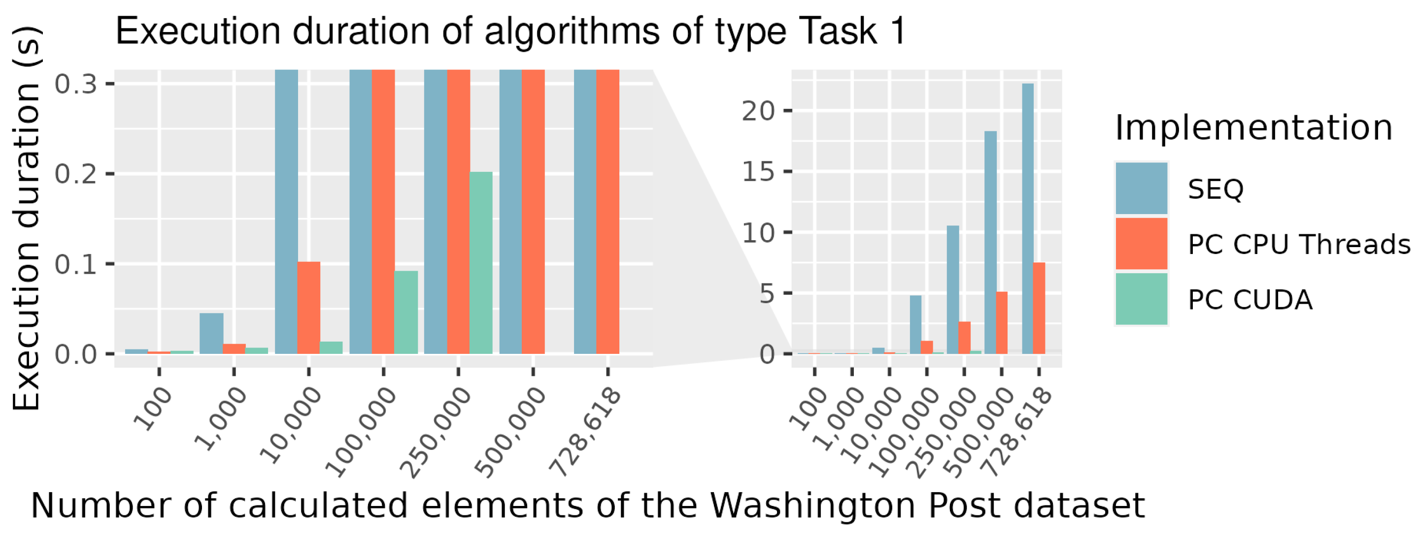
To measure a real-world speedup, we compared the runtime duration of the algorithm on different processors. The duration of execution was measured for the part of the metric calculation and for the entire processing, including the ordering of Graph Codes, as shown in Table 2 and visualized in Figure 9. As expected, the algorithm scales with input in an almost linear way. Tenfold the input takes tenfold the execution duration on the same system. For example, the CPU Parallel without Sort for 10,000 Graph Codes takes 0.1 s and a ten-times greater value of 1.021 s for 100,000 Graph Codes.
The processors used are different in multiple characteristics, so the execution durations cannot be compared one by one. However, they indicate that the CUDA CPU can process the same number of Graph Codes in a fraction of the time. Given the theoretical speedup of the algorithm explained in Section 3.4, it should primarily scale with the number of cores. Hence, we sought to prove this. We measured the performance on different CPUs and GPUs with a different number of cores. Again, the processors differed in clock rates and speed, but the focus was on the number of processor cores and the scalability of the algorithm.
5.2. Efficiency for High LOD
The mean number of features extracted from the WaPo collection is 39. We explored the behavior for cases with a higher LOD, based on artificially created Graph Codes of the same size. Therefore, we created Graph Codes with the same terms in the dictionary , following the same dimensions, dim, of the Graph Code matrix . To compare the results, we measured the runtime duration for shown in Table 5 and shown in Table 6. By comparing the runtime duration of CUDA and CUDA for 100 Graph Codes, for , CUDA performs better, but at , CUDA performs better. For the , CUDA also performs well for larger Graph Code collections, while CUDA and do not scale well. This behavior can be explained by the low GPU utilization of the sequential performance of PM calculations. Future research could examine whether the algorithm can perform better for a high LOD.
5.3. Impact of Graph Code Heterogeneity
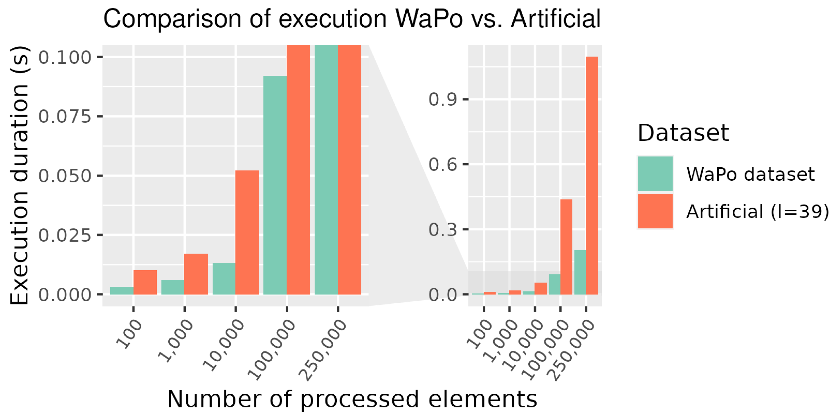
We explained the possible impact of heterogeneous Graph Codes on performance in Section 3.3. To evaluate the impact with real-world data, we performed an experiment and measured the runtime durations of CUDA with a subset of the WaPo dataset and artificial data. For artificial data, we generated comparable Graph Codes of . The results given in Table 7 and visualized in Figure 11 show that the heterogeneity of the input data does not necessarily have a negative impact on the duration of the runtime.
5.4. Summary
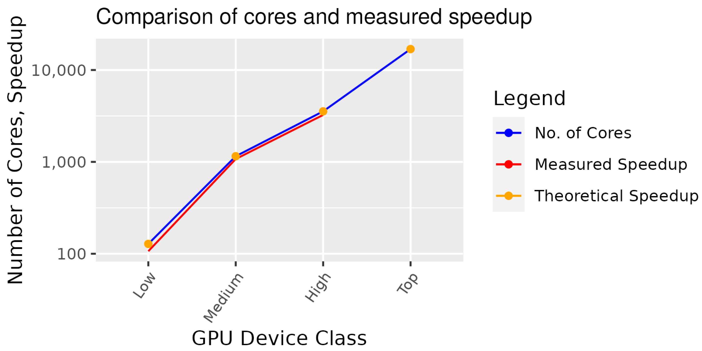
Our research focuses on the use case of similarity search in multimedia assets in multimedia collections. We wanted to examine the user experience of a Query by Example operation for large multimedia collections with a high LoD. High volumes and a high LoD result in high processing durations. Our experiments show that the parallel Graph Code similarity search can significantly reduce the execution duration. Our modeling and implementation have been validated by showing that the algorithm execution duration scales with the number of parallel processor cores. In our experiments, the algorithm on a medium GPU (see Table 1) achieved a speedup of 225 compared to a sequential execution on a medium CPU. These results lend clear support to the theoretical speedup on top-of-the-line GPUs.
6. Conclusions and Future Work
In this paper, we explained the difficulties for multimedia information retrieval introduced by growing multimedia collections and a high level of detail. Graph Codes are an efficient method to process multimedia content objects for use cases of similarity search. Processing large multimedia collections with sequential Graph Code algorithms still results in processing durations beyond the user-friendly margin of one second. We researched parallelization strategies for Graph Code algorithms, to improve the efficiency, which should lead to a better user experience. By applying decomposition methods, we modeled parallel versions of Graph Code algorithms. The characteristics of Graph Code metric calculation for the similarity search are good for scaling with both the number of Graph Codes to process and the number of processor cores used. We implemented a selection of the modeled algorithms for CUDA GPUs and CPUs with POSIX-Threads. The evaluation results prove the expected scaling behavior. A proven speedup of 225% could be measured. We integrated the implementation into GMAF and users observed less or even no loading times while searching for similarities.
In summary, massive speedups are possible on high-end GPUs and high speedups on CPUs. However, processing Graph Codes at the billion scale takes the processing time beyond the one-second margin. Based on the modeled algorithms, an implementation can be created for execution on multiple GPUs within a system or a distributed system. Such an implementation can probably achieve further acceleration.
As the evaluation has shown, a higher LOD results in larger dimensions of the Graph Codes and thus to a longer execution duration. Therefore, any measure that compacts the Graph Codes, or the originating MMFGs, will result in a better execution duration. One option to achieve this is the use of the compact SMMFGs. SMMFGs will improve the processing times with an acceptable loss of accuracy.
Future research could examine the performance of multi-GPU systems and the combined algorithm , which could lead to the speedup of plain for a high LOD.
Author Contributions
Conceptualization and methodology: P.S., S.W. and M.H. Software, validation, formal analysis, investigation, resources, data curation, writing: P.S. and S.W. Review, editing, and supervision: P.M.K., I.F. and M.H. All authors have read and agreed to the published version of the manuscript.
Funding
This research received no external funding.
Informed Consent Statement
Not applicable.
Data Availability Statement
The data presented in this study are openly available in [59].
Conflicts of Interest
The authors declare no conflict of interest.
References
- Richter, F. Smartphones Cause Photography Boom. 2017. Available online: https://0-www-statista-com.brum.beds.ac.uk/chart/10913/number-of-photos-taken-worldwide/ (accessed on 29 January 2023).
- DCTV Productions Comparing Streaming Services. (1 January 2022). Available online: http://web.archive.org/web/20220101112312/https://dejaview.news/comparing-streaming-services/ (accessed on 21 January 2023).
- DCTV Productions Comparing Streaming Services. (21 August 2022). Available online: http://web.archive.org/web/20220828145828/https://dejaview.news/comparing-streaming-services/ (accessed on 21 January 2023).
- Demner-Fushman, D.; Antani, S.; Simpson, M.; Thoma, G. Design and Development of a Multimodal Biomedical Information Retrieval System. J. Comput. Sci. Eng. 2012, 6, 168–177. [Google Scholar] [CrossRef] [Green Version]
- National Library of Medicine. What Is Open-i? Available online: https://openi.nlm.nih.gov/faq#collection (accessed on 21 January 2023).
- Jenik, C. A Minute on the Internet in 2021. Statista. 2022. Available online: https://0-www-statista-com.brum.beds.ac.uk/chart/25443/estimated-amount-of-data-created-on-the-internet-in-one-minute/ (accessed on 17 October 2022).
- Meta Platforms Ireland Limited. Instagram Homepage. 2022. Available online: https://www.instagram.com/ (accessed on 21 January 2023).
- Google. YouTube. Available online: http://www.youtube.com (accessed on 21 January 2023).
- Cloud Computing—Wikipedia. Page Version ID: 1128212267. 2022. Available online: https://en.wikipedia.org/w/index.php?title=Cloud_computing&oldid=1128212267 (accessed on 26 December 2022).
- Big Data—Wikipedia. Page Version ID: 1126395551. 2022. Available online: https://en.wikipedia.org/w/index.php?title=Big_data&oldid=1126395551 (accessed on 16 December 2022).
- Machine Learning—Wikipedia. Page Version ID1128287216. 2022. Available online: https://en.wikipedia.org/w/index.php?title=Machine_learning&oldid=1128287216 (accessed on 19 December 2022).
- Deep Learning. Wikipedia. Page Version ID1127713379. 2022. Available online: https://en.wikipedia.org/w/index.php?title=Deep_learning&oldid=1127713379 (accessed on 16 December 2022).
- Dasiopoulou, S.; Mezaris, V.; Kompatsiaris, I.; Papastathis, V.; Strintzis, M. Knowledge-Assisted Semantic Video Object Detection. IEEE Trans. Circuits Syst. Video Technol. 2005, 15, 1210–1224. Available online: http://0-ieeexplore-ieee-org.brum.beds.ac.uk/document/1512239/ (accessed on 21 January 2023). [CrossRef]
- Wagenpfeil, S.; Vu, B.; Mc Kevitt, P.; Hemmje, M. Fast and Effective Retrieval for Large Multimedia Collections. Big Data Cogn. Comput. 2021, 5. Available online: https://0-www-mdpi-com.brum.beds.ac.uk/2504-2289/5/3/33 (accessed on 11 October 2022). [CrossRef]
- Raieli, R. Multimedia Information Retrieval: Theory and Techniques; Chandos Publishing: Cambridge, UK, 2013; ISBN 978-1843347224. [Google Scholar]
- CXL.com. Reduce Your Server Response Time for Happy Users, Higher Rankings. 2021. Available online: https://cxl.com/blog/server-response-time/ (accessed on 12 October 2021).
- Kirk, D.; Hwu, W. Programming Massively Parallel Processors: A Hands-On Approach; Elsevier, Morgan Kaufmann: Amsterdam, The Netherlands, 2013. [Google Scholar]
- Apache™ Hadoop® Project Apache Hadoop. Available online: https://hadoop.apache.org/ (accessed on 13 January 2022).
- Singhal, A. Modern information retrieval: A brief overview. IEEE Data Eng. Bull. 2001, 24, 35–43. [Google Scholar]
- Davies, J.; Studer, R.; Warren, P. Semantic Web technologies: Trends and Research in Ontology-Based Systems; John Wiley & Sons: Hoboken, NJ, USA, 2006; OCLC: ocm64591941. [Google Scholar]
- Wagenpfeil, S.; McKevitt, P.; Hemmje, M. AI-Based Semantic Multimedia Indexing and Retrieval for Social Media on Smartphones. Information 2021, 12, 43. [Google Scholar] [CrossRef]
- Gurski, F.; Komander, D.; Rehs, C. On characterizations for subclasses of directed co-graphs. J. Comb. Optim. 2021, 41, 234–266. [Google Scholar] [CrossRef]
- Wagenpfeil, S.; Hemmje, M. Towards AI-based Semantic Multimedia Indexing and Retrieval for Social Media on Smartphones. In Proceedings of the 15th International Workshop on Semantic and Social Media Adaptation And Personalization (SMA), Zakynthos, Greece, 29–30 October 2020; pp. 1–9. [Google Scholar]
- Wagenpfeil, S.; Mc Kevitt, P.; Cheddad, A.; Hemmje, M. Explainable Multimedia Feature Fusion for Medical Applications. J. Imaging 2022, 8, 104. [Google Scholar] [CrossRef] [PubMed]
- Wagenpfeil, S.; McKevitt, P.; Hemmje, M. Graph Codes-2D Projections of Multimedia Feature Graphs for Fast and Effective Retrieval. ICIVR. 2021. Available online: https://publications.waset.org/vol/180 (accessed on 2 February 2022).
- Sciencedirect.com. Adjacency Matrix. 2020. Available online: https://0-www-sciencedirect-com.brum.beds.ac.uk/topics/mathematics/adjacency-matrix (accessed on 3 April 2023).
- Wagenpfeil, S.; Mc Kevitt, P.; Hemmje, M. Towards Automated Semantic Explainability of Multimedia Feature Graphs. Information 2021, 12, 502. Available online: https://0-www-mdpi-com.brum.beds.ac.uk/2078-2489/12/12/502. (accessed on 3 January 2023). [CrossRef]
- Asim, M.N.; Wasim, M.; Ghani Khan, M.U.; Mahmood, N.; Mahmood, W. The Use of Ontology in Retrieval: A Study on Textual. IEEE Access 2019, 7, 21662–21686. [Google Scholar] [CrossRef]
- Domingue, J.; Fensel, D.; Hendler, J.A. (Eds.) Introduction to the Semantic Web Technologies. In Handbook of Semantic Web Technologies; SpringerLink: Berlin, Germany, 2011. [Google Scholar] [CrossRef]
- W3C. SKOS Simple Knowledge Organisation System. 2021. Available online: https://www.w3.org/2004/02/skos/ (accessed on 2 February 2022).
- Silge, J.; Robinson, D. Text Mining with R: A Tidy Approach. (O’Reilly, 2017). OCLC: ocn993582128. Available online: https://www.tidytextmining.com/tfidf.html (accessed on 20 March 2023).
- Wagenpfeil, S. Smart Multimedia Information Retrieval. (University of Hagen, 2022). Available online: https://nbn-resolving.org/urn:nbn:de:hbz:708-dh11994 (accessed on 9 February 2023).
- Rauber, T.; Rünger, G. Parallel Programming; Springer: Berlin/Heidelberg, Germany, 2013; Section 3.3; pp. 98–112. [Google Scholar]
- Tanenbaum, A. Structured Computer Organization; Pearson Prentice Hall: Hoboken, NJ, USA, 2006; OCLC: Ocm57506907. [Google Scholar]
- Flynn, M. Very high-speed computing systems. Proc. IEEE 1966, 54, 1901–1909. Available online: http://0-ieeexplore-ieee-org.brum.beds.ac.uk/document/1447203/ (accessed on 17 December 2021). [CrossRef] [Green Version]
- Keckler, S.; Hofstee, H.; Olukotun, K. Multicore Processors and Systems; Springer: Berlin/Heidelberg, Germany, 2009. [Google Scholar]
- Apple Inc. M1 Pro and M1 Max. 2021. Available online: https://www.apple.com/newsroom/2021/10/introducing-m1-pro-and-m1-max-the-most-powerful-chips-apple-has-ever-built/ (accessed on 29 January 2023).
- Wikipedia. Apple A14. 2022. Available online: https://en.wikipedia.org/wiki/Apple_A14 (accessed on 12 January 2022).
- Intel Deutschland GmbH. Intel® Core™ i9-12900KF Processor. Available online: https://www.intel.de/content/www/de/de/products/sku/134600/intel-core-i912900kf-processor-30m-cache-up-to-5-20-ghz/specifications.html (accessed on 18 December 2021).
- Harish, P.; Narayanan, P. Accelerating large graph algorithms on the GPU using CUDA. In Proceedings of the High Performance Computing—HiPC 14th International Conference, Goa, India, 18–21 December 2007; pp. 197–208. [Google Scholar]
- Johnson, J.; Douze, M.; Jégou, H. Billion-scale similarity search with GPUs. arXiv 2017, arXiv:1702.08734. [Google Scholar] [CrossRef] [Green Version]
- Kusamura, Y.; Kozawa, Y.; Amagasa, T.; Kitagawa, H. GPU Acceleration of Content-Based Image Retrieval Based on SIFT Descriptors. In Proceedings of the 19th International Conference On Network-Based Information Systems (NBiS), Ostrava, Czech Republic, 7–9 September 2016; pp. 342–347. Available online: http://0-ieeexplore-ieee-org.brum.beds.ac.uk/document/7789781/ (accessed on 4 January 2022).
- Google Ireland Limited. TensorFlow Home Page. 2022. Available online: https://www.tensorflow.org/ (accessed on 18 December 2022).
- NVIDIA CUDA-Enabled Products. CUDA Zone. Available online: https://developer.nvidia.com/cuda-gpus (accessed on 18 December 2022).
- Grama, A. Introduction to Parallel Computing; Addison-Wesley: Boston, MA, USA, 2003. [Google Scholar]
- Rauber, T.; Rünger, G. Parallel Programming; Springer: Berlin/Heidelberg, Germany, 2013; Section 4.2.1; pp. 162–164. [Google Scholar]
- Amdahl, G. Validity of the Single Processor Approach to Achieving Large Scale Computing Capabilities, Reprinted from the AFIPS Conference Proceedings, Vol. 30 (Atlantic City, N.J., Apr. 18–20), AFIPS Press, Reston, Va., 1967, pp. 483–485, When Dr. Amdahl Was at International Business Machines Corporation, Sunnyvale, California. IEEE Solid-State Circuits Newsl. 2007, 12, 19–20. Available online: http://0-ieeexplore-ieee-org.brum.beds.ac.uk/document/4785615/ (accessed on 27 March 2022).
- Gustafson, J. Reevaluating Amdahl’s law. Commun. ACM 1988, 31, 532–533. [Google Scholar] [CrossRef] [Green Version]
- Norman, D.; Draper, S. User Centered System Design: New Perspectives on Human-Computer Interaction; L. Erlbaum Associates: Mahwah, NJ, USA, 1986. [Google Scholar]
- Object Management Group. Unified Modeling Language. 2011. Available online: https://www.omg.org/spec/UML/2.4.1/ (accessed on 29 April 2022).
- Harris, M. Optimizing parallel reduction in CUDA. Nvidia Dev. Technol. 2007, 2, 70. [Google Scholar]
- Manca, E.; Manconi, A.; Orro, A.; Armano, G.; Milanesi, L. CUDA-quicksort: An improved GPU-Based Implementation of Quicksort: CUDA-QUICKSORT. Concurr. Comput. Pract. Exp. 2016, 28, 21–43. [Google Scholar] [CrossRef]
- Harris, M.; Owens, J.; Patel, R.; Aaldavid; Yan, E.; Zhangyaobit; Sengupta, S.; Dan; Ap1. cudpp 2.2. (Zenodo,2014,8,31). Available online: https://zenodo.org/record/11548 (accessed on 17 September 2022).
- NVIDIA. NVIDIA H100 Tensor Core GPU. Available online: https://www.nvidia.com/en-us/data-center/h100/ (accessed on 3 January 2023).
- Sitaridi, E.; Ross, K. GPU-accelerated string matching for database applications. VLDB J. 2016, 25, 719–740. [Google Scholar] [CrossRef]
- Wikipedia Inverted index. Wikipedia. Page Version ID: 1137401637. 2023. Available online: https://en.wikipedia.org/w/index.php?title=Inverted_index&oldid=1137401637 (accessed on 19 February 2023).
- Chen, L.; Villa, O.; Krishnamoorthy, S.; Gao, G. Dynamic load balancing on single-and multi-GPU systems. In Proceedings of the International Symposium on Parallel and Distributed Processing (IPDPS), Atlanta, GA, USA, 19–23 April 2010. [Google Scholar]
- NIST. TREC Washington Post Corpus. Available online: https://trec.nist.gov/data/wapost/ (accessed on 6 March 2022).
- Steinert, P. marquies/gmaf-cuda. 2023. Available online: https://github.com/marquies/gmaf-cuda (accessed on 10 October 2022).
Figure 1.
A Minute on the Internet in 2021 [6].
Figure 1.
A Minute on the Internet in 2021 [6].

Figure 2.
Multimedia features represented as a Graph Code index (a–d) [27].
Figure 2.
Multimedia features represented as a Graph Code index (a–d) [27].

Figure 3.
UML use case diagram for similarity search with parallel execution.

Figure 4.
TDG for Task 1 and Task 3 with the and the as input.

Figure 5.
TDG for task 2a and task 2b with the value matrices as input.

Figure 6.
Comparison of (a) initial and (b) new parallel parts of the Graph Code algorithm in pseudocode. Colored items show tasks to decompose.
Figure 6.
Comparison of (a) initial and (b) new parallel parts of the Graph Code algorithm in pseudocode. Colored items show tasks to decompose.

Figure 7.
Task Dependency Diagram for Tasks 1–3.

Figure 8.
Combination overview of tasks and the resulting algorithms.

Figure 9.
Execution duration of algorithms of type Task 1.

Figure 10.
Comparison of speedup.

Figure 11.
Execution durations of real and artificial Graph Codes.


Table 1.
Hardware configurations of Central Processing Units (CPUs) and Graphical Processing Units (GPUs) used for evaluation.
Table 1.
Hardware configurations of Central Processing Units (CPUs) and Graphical Processing Units (GPUs) used for evaluation.
| Device Class | Low-End CPU | Low-End GPU | Medium CPU | Medium GPU | High-End CPU | High-End Desktop GPU | Top-of-the-Line GPU for Reference |
|---|---|---|---|---|---|---|---|
| Model name | Jetson Nano | Jetson Nano | Intel Core i5 | Nvidia GeFroce GTX 1060 3 GB | AWS c6a. 48xlarge | Nvidia RTX 3060 | Nvidia H100 80 GB PCIe |
| Processor | ARM Cortex-A57 MPCore | GM20B TM660M-A2 | i5-8500 | GP106/GP106-300-A1 | AMD EPYC | GA104 | H100 |
| Architecture | ARMv8-A64-bit | Maxwell | I686/Coffee Lake-S | Pascal | Zen | Ampere | Hopper |
| DRAM | 4096 MB | 4096 MB (shared) | 16 GB | 3 GB | 384 GB | 12 GB | 80 GB |
| CPU/GPU-clock | 1430 MHz | 640 MHz (921 MHz Boost) | 3 GHz | 1506 MHz (1708 MHz Boost) | Turbo 3.6 GZz | 1320 MHz (1777 MHz Boost) | 1830 MHz (1980 MHz Boost) |
| Cores | 4 CPU cores | 128 CUDA cores | 6 CPU cores | 1152 CUDA cores | 192 CPU cores | 3584 CUDA cores | 16,896 CUDA Cores |
Table 2.
Comparison of execution duration in seconds for Graph Code calculation and ordering for Sequential (), CPU Parallel (), and CUDA Parallel () of subsets of the WaPo dataset. Each measured the time with and without sorting.
Table 2.
Comparison of execution duration in seconds for Graph Code calculation and ordering for Sequential (), CPU Parallel (), and CUDA Parallel () of subsets of the WaPo dataset. Each measured the time with and without sorting.
| # GCs | CPU SEQ without Sort | CPU SEQ with Sort | CPU Par without Sort | CPU Par with Sort | CUDA Par without Sort | CUDA Par with Sort |
|---|---|---|---|---|---|---|
| [s] | [s] | [s] | [s] | [s] | [s] | |
| 100 | 0.005 | 0.005 | 0.002 | 0.002 | 0.003 | 0.003 |
| 1000 | 0.045 | 0.045 | 0.011 | 0.011 | 0.006 | 0.006 |
| 10,000 | 0.462 | 0.465 | 0.100 | 0.102 | 0.012 | 0.013 |
| 100,000 | 4.756 | 4.787 | 1.021 | 1.052 | 0.079 | 0.092 |
| 250,000 | 10.421 | 10.502 | 2.560 | 2.642 | 0.163 | 0.202 |
| 500,000 | 18.078 | 18.252 | 4.917 | 5.091 | — * | — * |
| 728,618 | 21.942 | 22.210 | 7.195 | 7.462 | — * | — * |
* out of memory.
Table 3.
Comparison of execution duration in seconds for Graph Code calculation and ordering for () on different CPUs.
Table 3.
Comparison of execution duration in seconds for Graph Code calculation and ordering for () on different CPUs.
| 10,000 | 50,000 | 100,000 | 200,000 | 400,000 | |
|---|---|---|---|---|---|
| Low-Level CPU (4 core) | 0.461 s | 2.338 s | 4.793 s | 9.798 s | 19.770 s |
| Medium CPU (6 core) | 0.102 s | 0.516 s | 1.053 s | 2.098 s | 4.088 s |
| High-Level CPU (192 core) | 0.018 s | 0.053 s | 0.091 s | 0.171 s | 0.326 s |
Table 4.
Comparison of execution duration in seconds for Graph Code calculation and ordering for () on different GPUs.
Table 4.
Comparison of execution duration in seconds for Graph Code calculation and ordering for () on different GPUs.
| 10,000 | 50,000 | 100,000 | 200,000 | 400,000 | |
|---|---|---|---|---|---|
| Low-Level GPU (128 Core) | 0.144 s | 0.467 s | 0.923 s | - * | - * |
| Medium GPU (1152 Core) | 0.013 s | 0.048 s | 0.092 s | 0.166 s | - * |
| High-Level GPU (3584 Core) | 0.004 s | 0.015 s | 0.030 s | 0.053 s | 0.110 s |
* out of memory.
Table 5.
Comparison of execution duration in seconds for Graph Code calculation for artificial Graph Codes of dim = 40.
Table 5.
Comparison of execution duration in seconds for Graph Code calculation for artificial Graph Codes of dim = 40.
| # GCs | CPU SEQ | CUDA PC | CUDA PM | CUDA PMPR |
|---|---|---|---|---|
| [s] | [s] | [s] | [s] | |
| 100 | 0.105 | 0.044 | 0.096 | 0.034 |
| 1000 | 1.050 | 0.043 | 0.888 | 0.247 |
| 10,000 | 10.512 | 0.096 | 8.905 | 2.372 |
| 100,000 | 105.956 | 0.562 | 88.529 | 23.286 |
Table 6.
Comparison of execution duration in seconds for Graph Code calculation for artificial Graph Codes of dim = 1000.
Table 6.
Comparison of execution duration in seconds for Graph Code calculation for artificial Graph Codes of dim = 1000.
| # GCs | CUDA PC | CUDA PM | CUDA PMPR |
|---|---|---|---|
| [s] | [s] | [s] | |
| 100 | 121.167 | 2.863 | 2.208 |
| 1000 | 387.565 | 28.334 | 21.502 |
Table 7.
Comparison of execution duration in seconds for Graph Code calculation for artificial Graph Codes of dim = 39.
Table 7.
Comparison of execution duration in seconds for Graph Code calculation for artificial Graph Codes of dim = 39.
| # GCs | CPU SEQ | CPU PC | CPU PC |
|---|---|---|---|
| [s] | [s] | [s] | |
| 100 | 0.098 | 0.022 | 0.010 |
| 1000 | 0.983 | 0.222 | 0.017 |
| 10,000 | 9.796 | 2.248 | 0.052 |
| 100,000 | 98.389 | 22.080 | 0.437 |
| 250,000 | 244.893 | 54.606 | 1.095 |
| 500,000 | 490.977 | 108.641 | 2.187 |
| 728,618 | - | - | 3.194 |
Disclaimer/Publisher’s Note: The statements, opinions and data contained in all publications are solely those of the individual author(s) and contributor(s) and not of MDPI and/or the editor(s). MDPI and/or the editor(s) disclaim responsibility for any injury to people or property resulting from any ideas, methods, instructions or products referred to in the content. |
© 2023 by the authors. Licensee MDPI, Basel, Switzerland. This article is an open access article distributed under the terms and conditions of the Creative Commons Attribution (CC BY) license (https://creativecommons.org/licenses/by/4.0/).
Share and Cite
MDPI and ACS Style
Steinert, P.; Wagenpfeil, S.; Mc Kevitt, P.; Frommholz, I.; Hemmje, M. Parallelization Strategies for Graph-Code-Based Similarity Search. Big Data Cogn. Comput. 2023, 7, 70. https://0-doi-org.brum.beds.ac.uk/10.3390/bdcc7020070
AMA Style
Steinert P, Wagenpfeil S, Mc Kevitt P, Frommholz I, Hemmje M. Parallelization Strategies for Graph-Code-Based Similarity Search. Big Data and Cognitive Computing. 2023; 7(2):70. https://0-doi-org.brum.beds.ac.uk/10.3390/bdcc7020070
Chicago/Turabian StyleSteinert, Patrick, Stefan Wagenpfeil, Paul Mc Kevitt, Ingo Frommholz, and Matthias Hemmje. 2023. "Parallelization Strategies for Graph-Code-Based Similarity Search" Big Data and Cognitive Computing 7, no. 2: 70. https://0-doi-org.brum.beds.ac.uk/10.3390/bdcc7020070