Design of Cascaded and Shifted Fractional-Order Lead Compensators for Plants with Monotonically Increasing Lags


Department of Electrical and Information Engineering, Polytechnic University of Bari, Via E. Orabona, 4, I-70125 Bari, Italy
Fractal Fract. 2020, 4(3), 37; https://0-doi-org.brum.beds.ac.uk/10.3390/fractalfract4030037
Submission received: 2 July 2020
/
Revised: 21 July 2020
/
Accepted: 23 July 2020
/
Published: 27 July 2020
(This article belongs to the Special Issue Fractional Calculus in Control and Modelling)
Abstract
:This paper concerns cascaded, shifted, fractional-order, lead compensators made by the serial connection of two stages introducing their respective phase leads in shifted adjacent frequency ranges. Adding up leads in these intervals gives a flat phase in a wide frequency range. Moreover, the simple elements of the cascade can be easily realized by rational transfer functions. On this basis, a method is proposed in order to design a robust controller for a class of benchmark plants that are difficult to compensate due to monotonically increasing lags. The simulation experiments show the efficiency, performance and robustness of the approach.
1. Introduction
Fractional calculus is an old field of science that, based on the initial idea of generalizing derivatives with integer order to derivatives with non-integer order, has given rise to many results in the pure field of mathematics [1,2,3,4]. However, today the field has tremendously grown and has many and various applications in science and engineering [5,6,7,8], such that even modeling, analysis, and control of complex systems requiring a multi-disciplinary approach [9,10] can be approached by fractional calculus tools [11,12,13].
In the specific field of automatic control, it is now more than two decades since the influential book [14] reported that the of the control loops worldwide were of Proportional-Integral-Derivative (PID) type. Today, the technological trends and the increasing demand of better tuning make it clear that the PID controllers are still a subject of intensive research. Hence, following the boost to innovation in the late twentieth century, the fractional-order controllers (FOCs) are also proposed for industrial applications [15,16,17,18,19,20,21,22].
The first attempt to classify the FOCs used in process applications mentioned four types [23]: the TID controller [24], the CRONE controller [25,26], the controller [27], and the fractional lead-lag compensator [28]. All share the same idea of using irrational compensators ensuring flat phase in Bode plots. Namely, if the phase derivative with respect to the frequency is zero (or nearly zero), then robustness to gain variations and iso-damping behavior of the step response is achieved. Hence, ensuring flat phase property is a main reason justifying the interest for FOCs.
In the years following the publication of [23], a great effort has been made to develop efficient FOC tuning procedures in both the frequency and time domain. A noticeable, present-day research direction in tuning approaches opts for optimization techniques with constraints that are expressed by time-domain specifications (rise time, settling time, percentage overshoot, error indices, etc.) or by frequency-domain specifications (phase/gain margin, crossover frequency, bandwidth, sensitivity magnitudes, etc.). For example, the tuning of a fractional-order PID (FPID) controlling a first-order plus delay-time process is converted into an optimization problem [17,29]. In other cases, the tuning is based on parameter searching in a multidimensional space [30]. In addition, as regards the time-domain optimization approaches, many authors employed evolutionary algorithms for tuning FPID controllers. For example, they applied Particular Swarm Optimization (PSO) or Genetic Algorithms to minimize the Integral Time Absolute Error (ITAE) [31,32] or a combination of the ITAE and the Integral Square Error (ISE) [33] or the integral absolute error (IAE) [34] or a combination of the integral gain and closed-loop system bandwidth [35]. Additionally, a combination of differential evolution and PSO was proposed to design and realize FOC based on time-domain performance specifications [36].
Clearly, the drawback of all the optimization-based tuning procedures is that they should be repeated for any specific model that one takes into account. However, in practice, control engineers need easy-to-apply, efficient tuning rules. For this reason, some attempts generalized the Ziegler and Nychols rules to FPID tuning [37,38]. New formulas also extended the Symmetrical Optimum approach [14] to tune the fractional-order PI (FPI), also named PI controller, in positions control of a class of electromechanical systems [39]. To overcome the difficulties, the research on FPIDs developed empirical tuning rules and some auto-tuning approaches [17,39,40,41,42,43,44,45,46,47,48]. Whatever tuning approach is chosen, the practical implementation of FPID is a critical issue. Namely, the fractional-order transfer functions (TFs) of the FOC frequently require to be approximated by high-order rational TFs.
On the basis of the above considerations, this paper considers the Cascaded, Shifted, Fractional-order, LEad Compensators (CS-FLECs), a new class of compensators enjoying the following characteristics:
- (A)
- The CS-FLECs are multistage compensators, in which each stage is in its turn a fractional-order lead compensator (FLEC). Each FLEC stage is frequency-scaled with respect to the previous one, so that it provides phase lead values with a nearly flat phase on an adjacent interval. When compared with a cascade of identical FLECs that are superposed on the same frequency interval, a CS-FLEC exhibits a nearly flat phase in a much larger frequency interval. This is a direct result of the serial structure of the shifted stages.
- (B)
- To implement a CS-FLEC, each stage needs a rational TF approximation. As the paper shows, a second-order TF provides a satisfactory approximation in the frequency interval of each stage of the cascade. The values of the coefficients in each second-order TF ensure low sensitivity in both analogue and digital realizations.
- (C)
- The paper shows how to apply CS-FLEC structures to compensate a class of plants that are notoriously difficult to control [49,50]. The approach is especially suited for plants that are characterized by monotonically increasing lags. The fundamental ideas underlying the design pattern are simple and refer to formulas based on the properties of the CS-FLEC. The paper also brings out the limits of the CS-FLEC in controlling the chosen benchmarks.
The organization of the paper is the following. Section 2 introduces the CS-FLEC controller and illustrates its properties. Section 3 provides a new and easy method for implementing rational, low-order TF of these controllers. Section 4 describes the procedure to design a CS-FLEC. Section 5 presents and discusses two case-studies that show how CS-FLECs control classes of processes, reported as benchmarks by the technical literature. Section 6 provides the conclusions.
2. Cascaded, Shifted, Fractional-Order Lead Compensator
This section describes the CS-FLEC that is composed by two elements, indicated by and , which are defined in shifted, partially overlapping, intervals of the frequency axis.
2.1. The First Compensator Stage
The basic element of the proposed CS-FLEC is the first compensator, that is described as
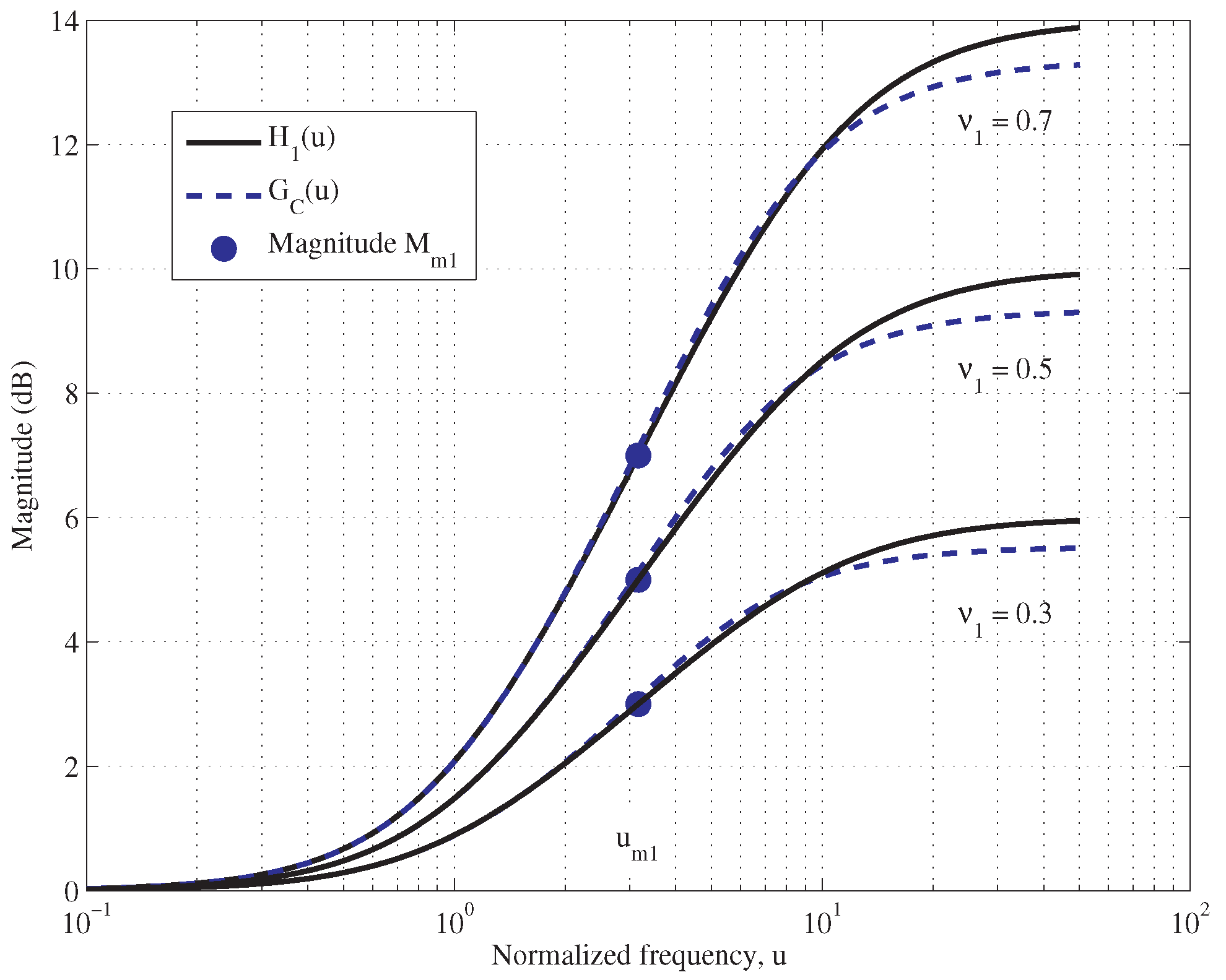
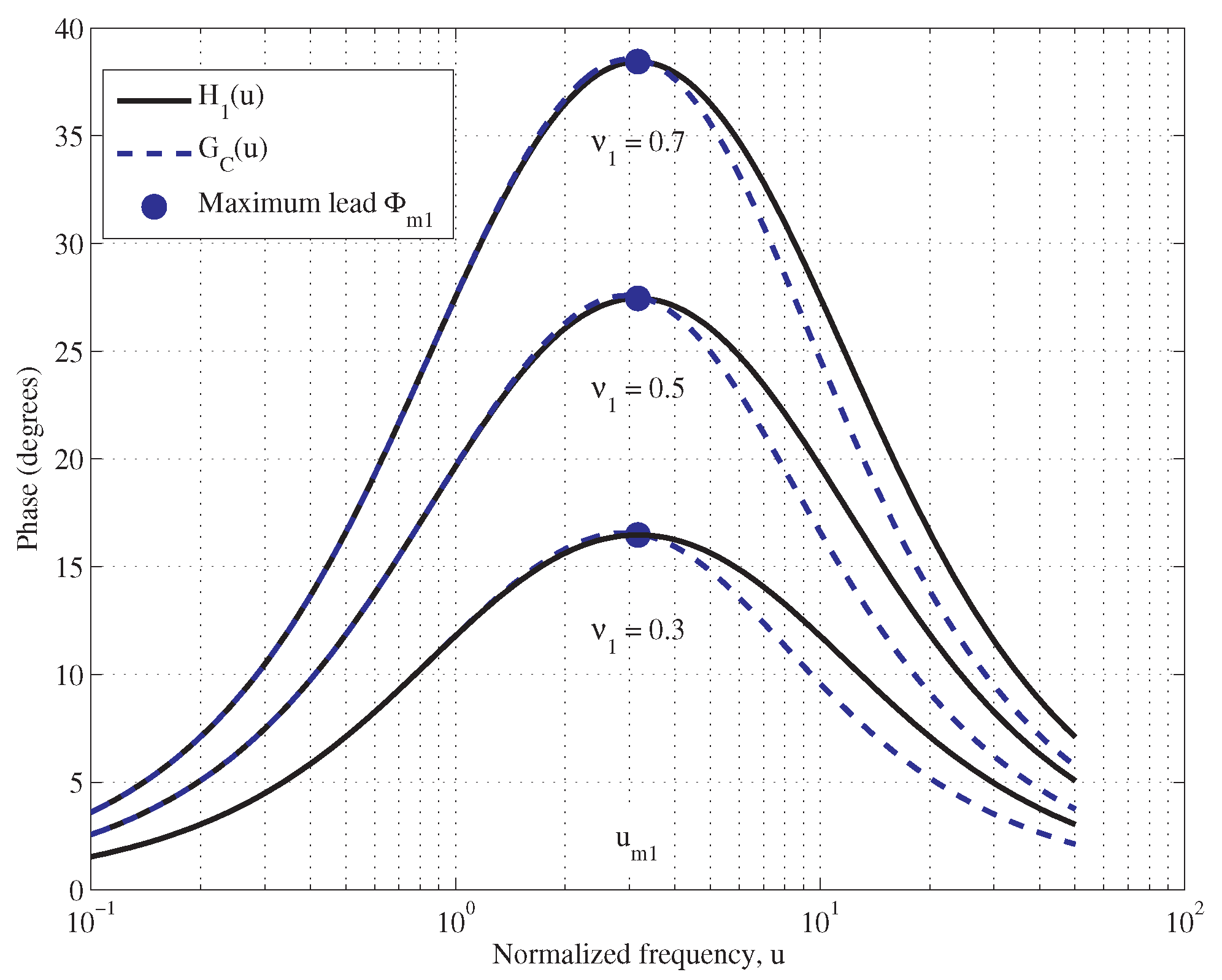
with and when considering a fractional-order lead compensator (FLEC) [40]. The symbols and represent the time constant and the fractional order, respectively. Now, put to recall the frequency key features of a FLEC. It is well known that the maximum phase lead of is obtained at the geometric mean of and [27,51]:
In this frequency, the magnitude, say , and the phase, , are:
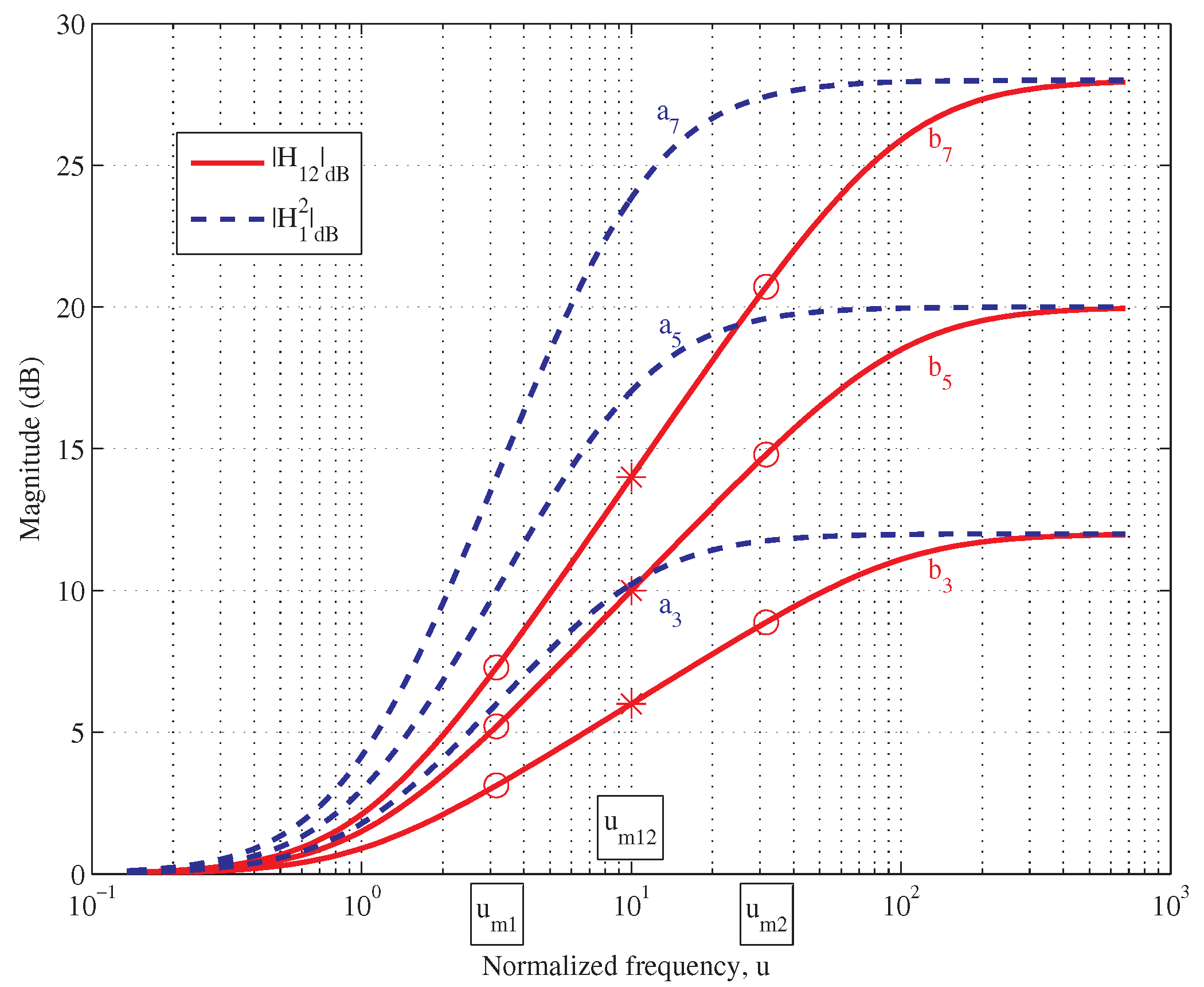
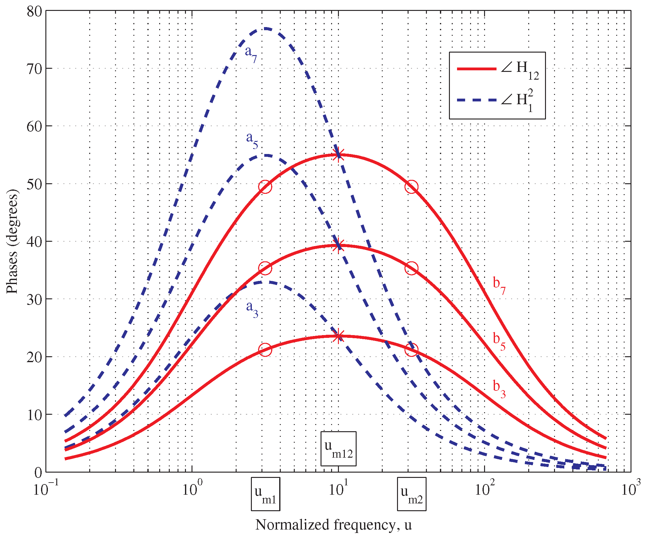
Figure 1 and Figure 2 show, in solid lines, the magnitude and phase plots of the normalized frequency response of the compensator , where is a normalized frequency, for , and . The circles represent the pairs and corresponding to the assigned values of .
Higher values of provide higher phase leads while the lower ones lead to a flatter behavior of the phase plots.
By Equation (4), the maximum phase lead depends on and , whose values dictate the amount of the introduced phase lead. For integer-order compensators (), many authors usually consider values of in the range between and [52], in particular . Subsequently, with , the Equation (4) gives . Accordingly, integer-order compensators consisting of a series of two stages with the same zero-pole pair provide greater phase leads. In this conventional structures, the serial stages have equal characteristics and, at each frequency, provide equal contributions to the resulting phase lead.
2.2. The Second Compensator Stage
The proposed structure differs from the conventional one. A CS-FLEC, indeed, is a cascade of two FLECs with the same Bode plots, but the position on the -axis of the second stage is shifted with respect to the first one. The shifting amount is established to make the phase of each FLEC element dominate on its nearly flat phase frequency interval. The resulting lead network, i.e., the CS-FLEC, has a relatively low order and enjoys the flat phase property in a large frequency band. In details, once the parameters of have been chosen, the second FLEC, say , is obtained by using in place of and by scaling with the substitution , where is used as scaling factor:
In this way, the frequencies delimiting the flatness interval of the CS-FLEC can be fixed in terms of the features of the two stages in the series. Namely, it is easy to show that gives its maximum phase lead at the frequency
and
Moreover, comparing Equations (3), (4), (7), and (8), and using yields: , and, for any frequency , . Figure 3 and Figure 4 show the magnitude and phase plots for the analogue compensators and (see dashed and dash-dotted lines, respectively). For clarity reasons, these figures only use the values . The curves assume and they are drawn in terms of the nondimensional frequency , so that and correspond to the maximum leads the two stages respectively provide.
2.3. The Serial Compensator
With the chosen parameters and , the series connection of the two compensators is equivalent to a single unit:
By using , it follows
and, by Equations (2) and (9), the maximum phase lead is obtained at the geometric mean of the new break-away frequencies:
At , the magnitude is
and the maximum phase lead is
The frequencies and define the interval , where the phase is nearly flat (see Figure 4) and where the magnitude characteristic of follows a nearly straight pattern (solid lines in Figure 3). Beyond this range, the magnitude plot tends to a horizontal line and the CS-FLEC provides the maximum magnitude for each value of .
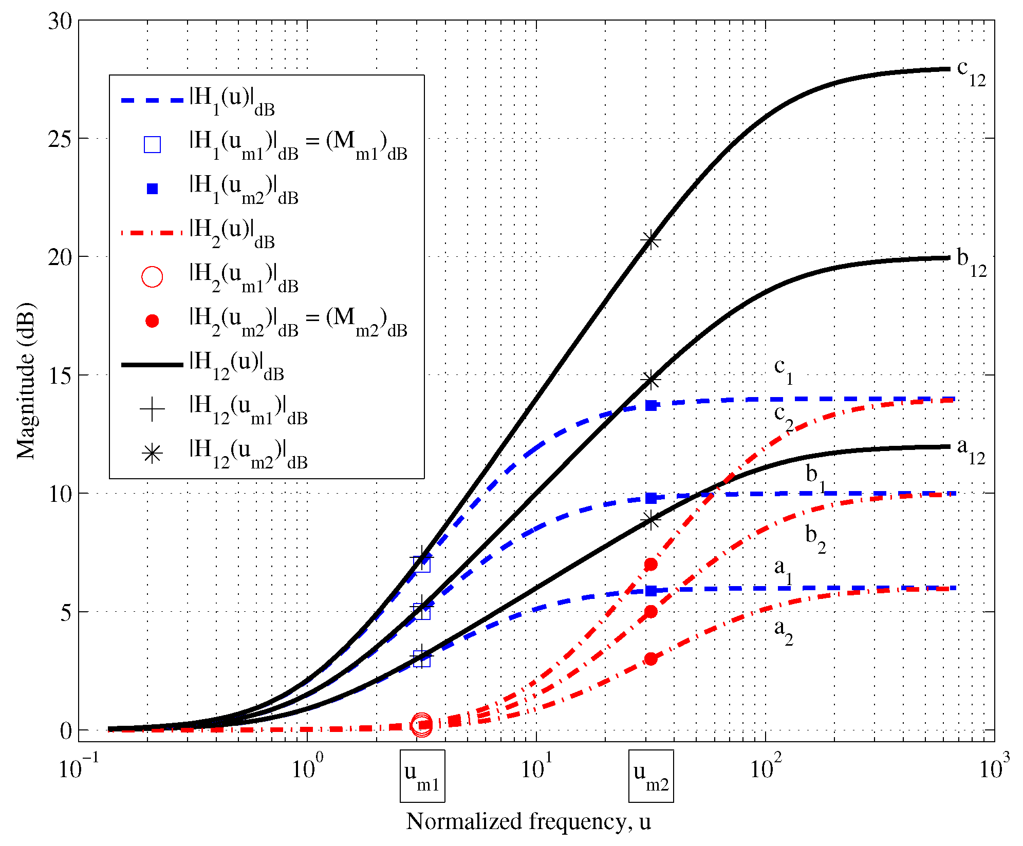
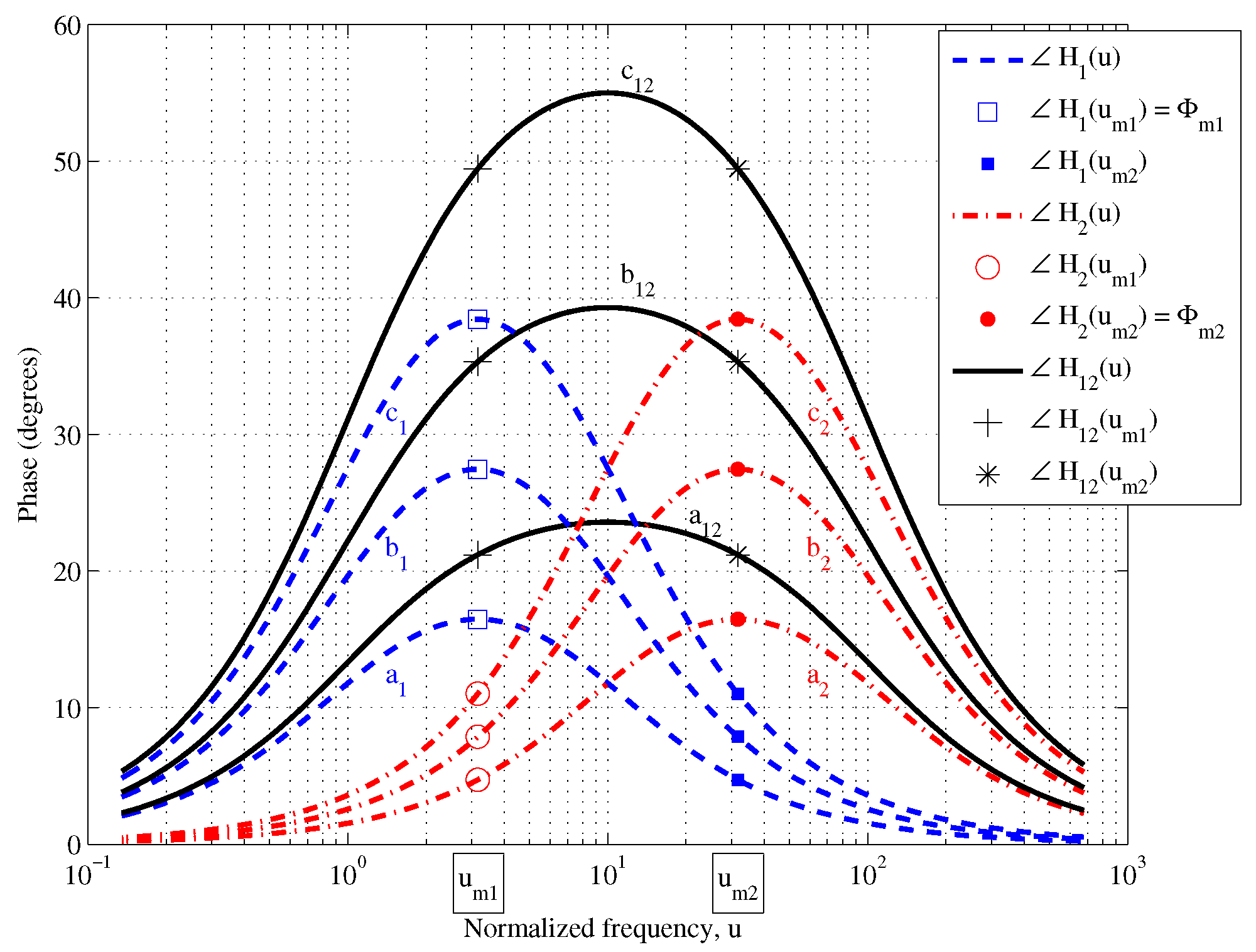
Figure 5 and Figure 6 compare the Bode diagrams of the CS-FLEC specified by with the Bode diagrams of the conventional series of two identical FLECs, specified by . The cases with and are considered. Compensators and provide the same high-frequency gain, even if the magnitude of the former increases more gradually than the magnitude of the latter. Finally, by Equations (4) and (13), the maximum phase lead given by is that is greater than , which is provided by . However, the phase characteristics of are flatter than those of . Moreover, the slopes of the plots of and , evaluated on the right (or left) of and , respectively, are measures of the flatness of the phase. Because the decreasing of around is more rapid than the falling of around , the latter plot is flatter than the former one.
3. Realization
Because the CS-FLEC is an irrational function, its implementation needs a rational integer-order TF approximation. Literature shows many frequency domain approaches to approximate irrational operators and functions, starting with early contributions like [53,54,55]. The most referred methods are the Oustaloup recursive approximation (ORA) [56] and the modified Oustaloup technique [57]. They employ popular formulas to alternate zeros and poles of the rational transfer function in the frequency interval of practical interest, but they often determine approximations of very high order. Methods that are based on continued fraction expansions (CFE), interpolation, and curve-fitting methods are also important [58,59], and even the Matsuda approach, which is one of the best known, combines CFE and a fitting technique [55]. Moreover, CFE-based methods are preferred to those using power series expansions, because better convergence properties imply less coefficients to obtain a good approximation [58]. A good review of the basic approaches and techniques was given by [60].
In recent years, researchers proposed several other techniques, among which one may consider [61,62,63,64,65,66,67]. Namely, it was pointed out that fractional-order lead compensators found difficult application in industry, because it is difficult to obtain the desired functions with the commercially available electronic components, such that special methods that are based on operational amplifiers and field programmable analog arrays should be used [61]. In [63], the authors design two fractional-order lead-lag compensators to control a benchmark refrigeration system (the PID2018 benchmark challenge) such that a more aggressive response is obtained. In this case, approximation is simply performed via the Matlab command fitmagfrd from the Robust Control Toolbox. Other peculiar techniques could take advantage from orthonormal rational basis functions, which can be used to improve fitting and approximation of frequency response, as shown in [64]. Some other authors proposed curve fitting techniques (with built-in Matlab functions) that use frequency response data of fractional-order operators to improve the ORA, the modified ORA, or the Matsuda approximation [65]. A Scilab Based Toolbox is also available for fractional-order operators, transfer functions, filters, and controllers [66]. Finally, the recent work presented in [67] implements fractional-order lead/lag compensators using Operational Transconductance Amplifiers as active blocks. To this aim, the authors consider a Padé approximation proposed in [68] and obtain the same form of realization for the two types of fractional transfer functions, which allows them to use the same active core and to electronically tune the characteristics of the compensators. Contributions for the discretization and digital implementation of fractional functions are many and beyond the scope of this paper.
Here, each stage of the CS-FLEC is approximated by a second-order rational TF, which gives sufficient accuracy in the frequency range of interest. Note that a low-order implementation is advantageous, because the changes of the coefficients due to passive component tolerances (analogue implementation) or to the limitations of microprocessor words and the quantization effects (digital implementation) are quite contained [69,70], such that a low sensitivity to parameter variations is obtained.
The realization method leads to the following expression of the approximated FLEC (see Appendix A)
with
where , , [71] and
where , .
Figure 1 and Figure 2 show in dashed lines magnitude and phase plots of a second-order realization of the FLEC. The approximation accuracy is satisfactory in the frequency range of interest for the single (irrational) stage FLEC. The plots in Figure 1 and Figure 2 show that both the magnitude and the phase practically coincide with the plots representing the irrational FLEC in the frequency interval , which is important for compensation. Instead, for , the approximation gets worse. On the other hand, for practical purpose, it can be easily verified that higher-order, rational TFs do not significantly improve the approximation in the frequency range where a nearly flat phase is achieved.
Now, consider the rational TFs indicated by and , respectively representing the second-order realizations of and . Subsequently, the cascade provides a fourth-order realization of .
4. The Design Method
To achieve robustness to gain variations, the phase margin must be nearly constant in a frequency interval around the gain crossover frequency of the compensated system, . That is, the tangent line to the curve of the phase angle of the open-loop TF should have a small slope in a given range around . Even if this curve is not completely flat, the robustness can be ensured if is greater than an established minimum value for a wide frequency spread around . The width of the range is also important to guarantee robustness.
Hence, let be the open-loop TF, including the controller and the plant . To introduce the design method, the following essential facts clarify the objectives, specify the assumptions, and provide some advice.
- a.
- The features of the CS-FLEC are suitable for controlling plants with phase lags which are monotonic increasing with the frequency . Afterwards, putting , the phase margin of the plant at its gain crossover frequency , , is often negative.
- b.
- The compensator will introduce a phase lead compensating the lag of the plant so as to obtain the flattest possible phase trend in the range surrounding , i.e., the gain crossover frequency of . However, the CS-FLEC shifts to the right of . Accordingly, if and decrease sharply beyond , cannot introduce leads balancing the greater lags (see the plant phase diagrams in Figure 7 and Figure 8). For this reason, the value of gain must be properly adjusted to make or even if these frequencies are not too far from each other.
- c.
- To satisfy the previous requirements, is chosen by composing and , having phase plots in shifted frequency ranges. More preciselywhere and is the scaling factor. The strategy is that introduces the larger lead amount, while improves the flatness. It holds .
- d.
- The compensated system must show an adequate phase margin (e.g., ) with a phase decay rate beyond that is less than that of the corresponding plant. Finally, from must be , without excessively reducing the system bandwidth.
- e.
- Let and define the slope . Afterwards, to improve the robustness to gain variations in a frequency range around , the slope must decrease as much as possible. Since the value of estimates the robustness to gain variations, some approaches are proposed for evaluating this parameter [43]. In the present case, simple calculations give (see Appendix B)It can be verified that , , and make , where provides the plant slope.
To sum up, the parameters of the compensator to be determined are , , , and , while and are known from the start. The procedure to set the parameters is specified, as follows.
- I.
- By Equation (2), the time constant can be easily determined in terms of , the frequency where occurs. However, due to the lead contribution of , the controller reaches the maximum phase lead at frequency . Hence, to put , is chosen, so that with . The parameter h can be determined by few successive attempts. A first one can be .
- II.
- To set and , the phase margin specification on is considered. Hence, since and , the following approximate relation can be used:where by Equation (4) and is computed by Equation (5). Note that, if the plant shows a phase lag rapidly increasing with the frequency, can be negative. Moreover, it is suitable to choose , otherwise large values for would increase the magnitude of , that shifts the crossover of too far beyond . A rule of thumb, which is tested by numerical experiments, indicates . Moreover, Equation (19) shows that values of allow to compensate in order to obtain and achieve a right compromise between robustness and dynamic response.
- III.
- is set, so that . The gain crossover frequency , indeed, can also assume values that are less than . This choice is convenient if a greater phase margin is required and if decreases. However, must be quite close (to the left) to .
- IV.
- The performance is verified. If specifications are not met, then the procedure must be repeated by going back to step I. (or III.), decreasing (or ), then changing and so on.
Note that the design pattern refers to the irrational TF . Usually, the step response characterizes the system performance in terms of rise time , maximum overshoot , and settling time (if necessary). To establish a total reliance on computer simulation, is replaced by its rational approximation according to the approach presented in Section 3, thus providing a rational approximation for .
Finally, for comparison purpose, one can design a cascade of two identical FLECs, namely , where is specified by Equation (1). In this case, the maximum phase lead is at . By using the same values of , , and , a procedure that is similar to that for the CS-FLEC can be followed. At step I, by putting with (e.g., ) and using Equation (2), the time constant is determined in terms of and . At step II, the relation provides . At step III, is set so that . At step IV, performance is verified.
5. Two Illustrative Benchmark Examples
The design approach is illustrated by two meaningful and demonstrative benchmarks taken from the literature.
5.1. First Example
Consider the plant model
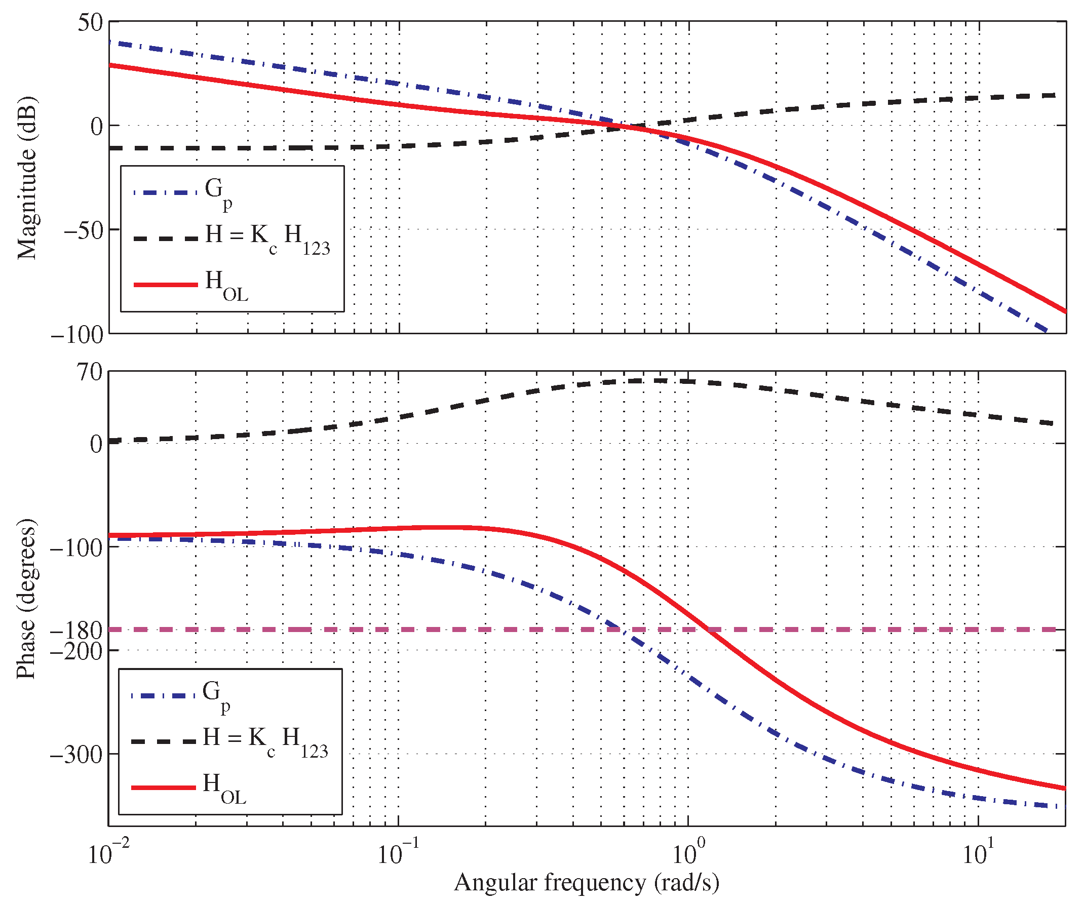
that is a benchmark proposed by [50]. In Figure 7, the Bode diagrams give with then and .
The design method is applied with . The specifications are a phase margin to ensure stability, despite plant gain and parameter variations. The overshoot in the unit step response of the closed-loop system should not be much higher than .
One choice of the CS-FLEC parameter set comes from a first iteration of the design method and is as follows:
- –
- Step I: s
- –
- Step II: and
- –
- Step III:
- –
- Step IV: the obtained phase margin is in rad/s. The slope of the phase plot is . The step response shows a overshoot and settling time of s.
These results could be satisfactory, however a second iteration gives:
- –
- Step I: s
- –
- Step II: and
- –
- Step III:
- –
- Step IV: the obtained phase margin is in rad/s. Moreover, , which is a good improvement. The step response shows a overshoot and settling time of s.
The controller is realized, as follows:
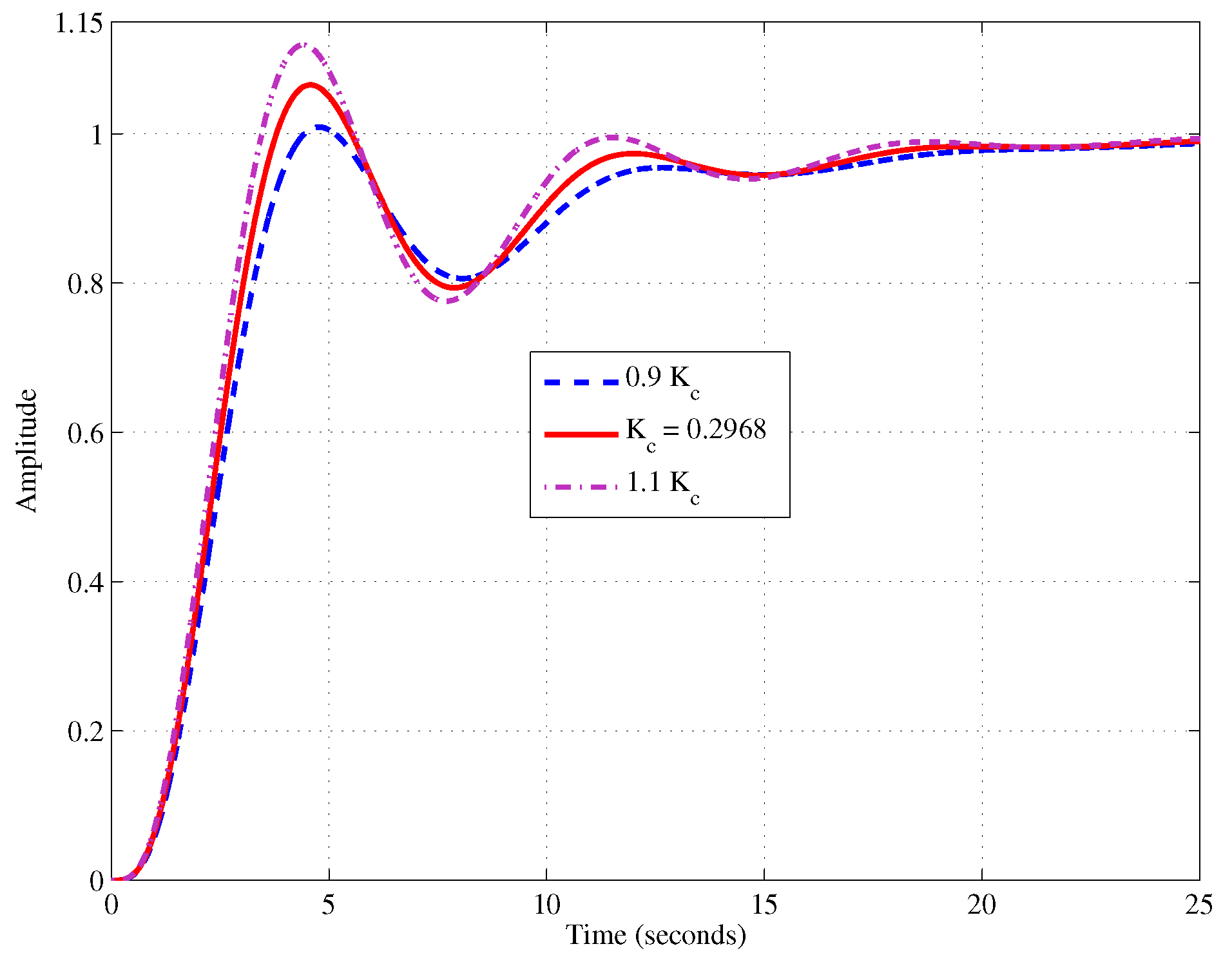
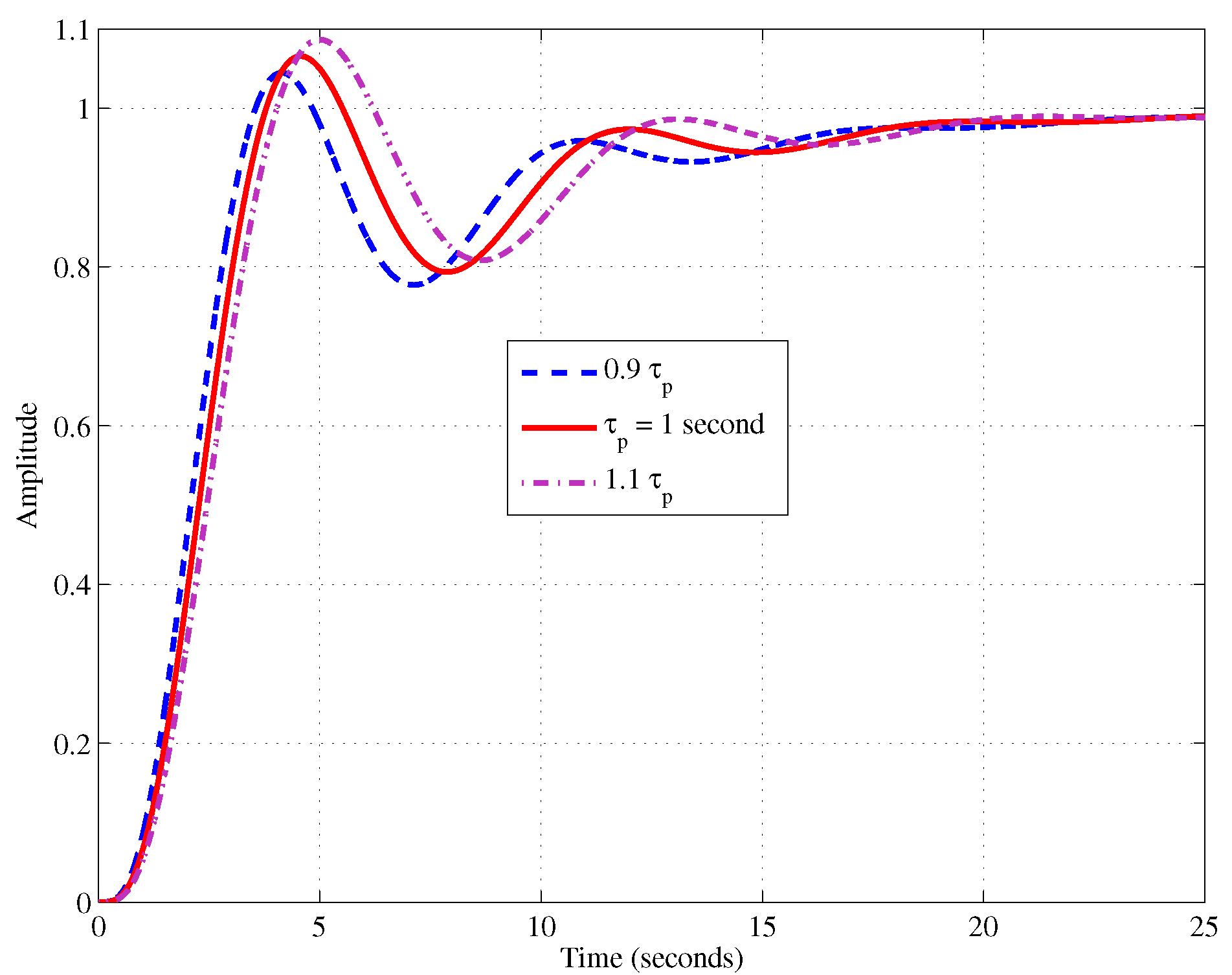
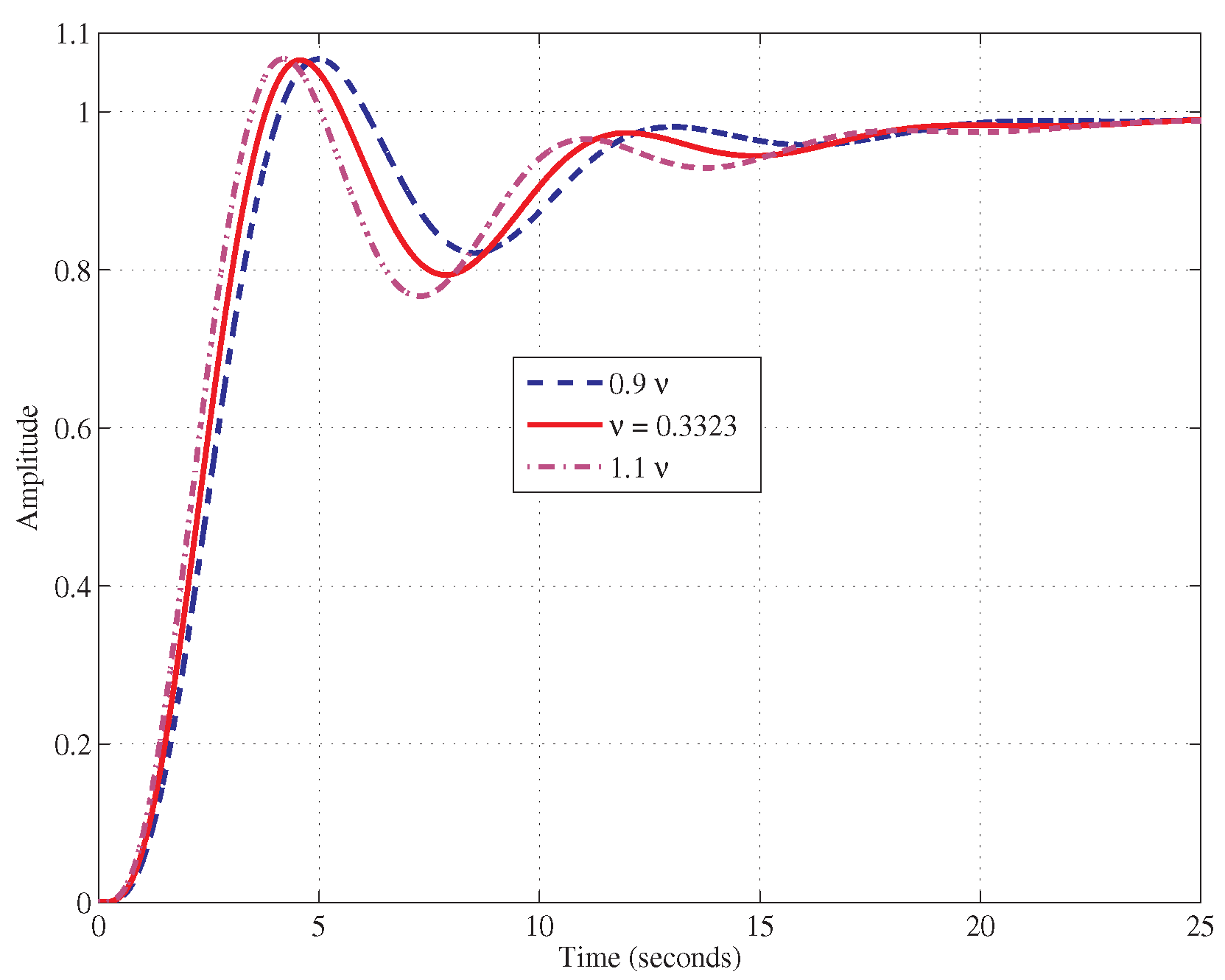
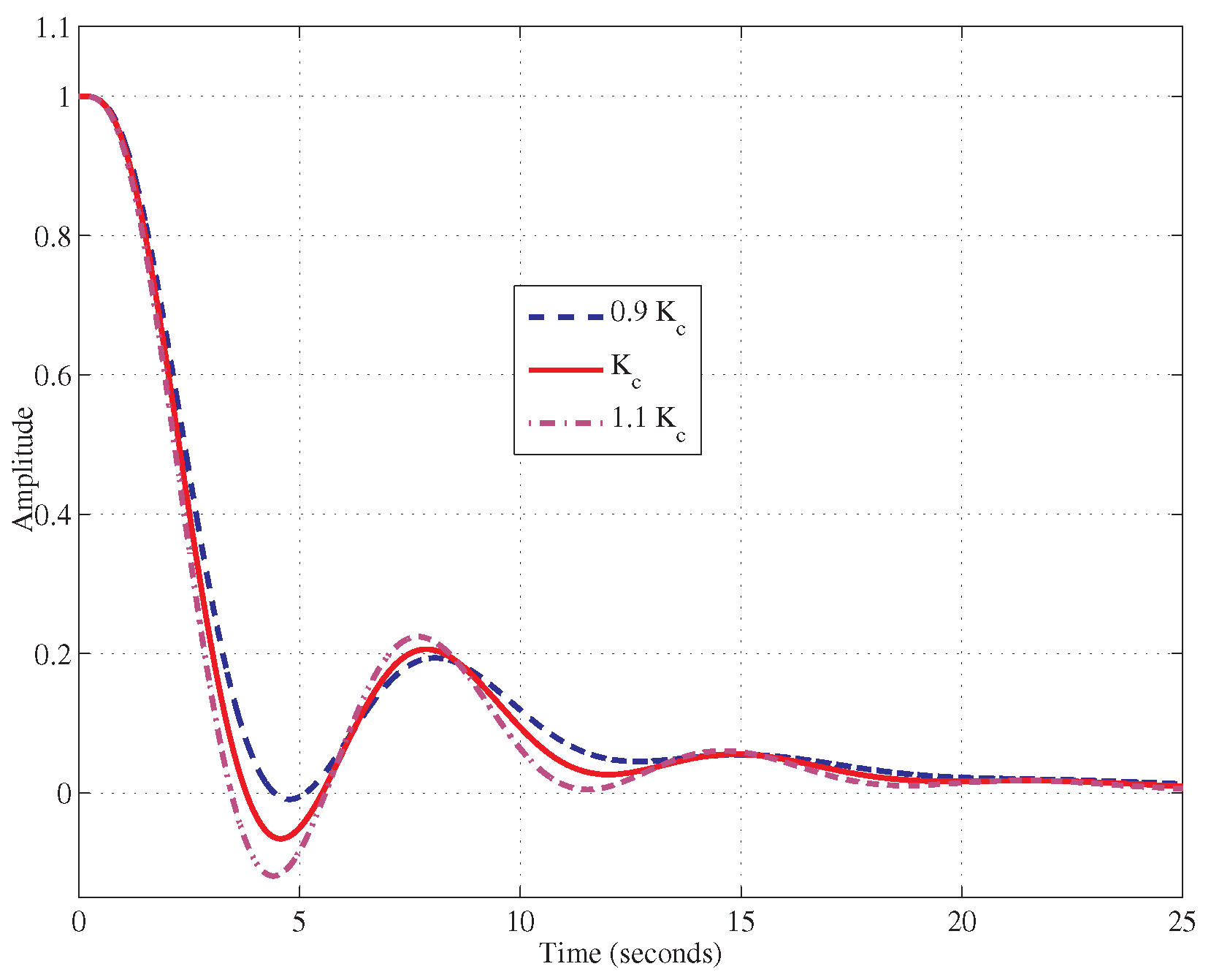
Table 1 reports the performance indexes when or the plant time constant or the fractional order change by a amount with respect to their nominal values , s, and . and take the values assigned by the design. See Figure 9, Figure 10 and Figure 11 for the responses. Note that, here, the rise time is required for the response to rise from to of the steady-state value. The settling time is defined for a requirement. In all cases, is contained and stays below and it does not change in a significant way. The settling time has satisfactory values. All of the responses show undershoots that increase with .
To validate an auto-tuning technique, the authors of [43] proposed simulation results referred to the process (20) controlled by a FPID tuned by an iso-damping approach. The specifications were the desired “tangent frequency” rad/s and the “tangent phase margin” at , i.e., . Subsequently, the Bode plots in [43] showed a flat phase curve near (at the peak of the phase plot). Hence, the step responses remained nearly constant with respect to the gain variation, thus showing robustness. The overshoot was roughly . The design approach proposed here gives rad/s with a phase margin of . Moreover, limited changes of the step responses occur due to the gain (or other parametric) variations and the overshoots are below (see Figure 9, Figure 10 and Figure 11 and Table 1).
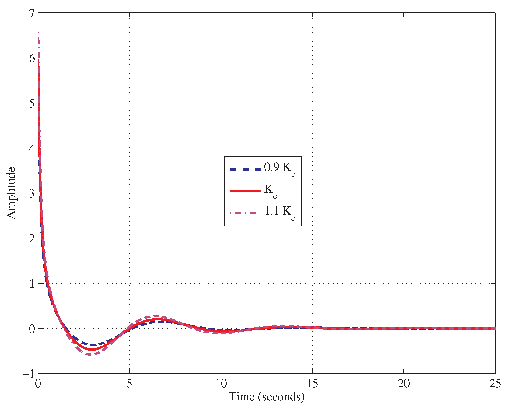
Finally, the control variable and the unit step disturbance rejection are illustrated in Figure 12 and Figure 13 for variations of . The results obtained in case or change do not affect the performance in a substantially different way. Figure 12 shows that high initial values of the control variable are obtained. However, the amplitude of the manipulated variable is usually subject to limitations deliberately placed on actuators for accounting the limited power available to the control system and avoiding damages to the process [72].
The design of two identical FLECs gives the following results:
- –
- Step I: s
- –
- Step II:
- –
- Step III:
- –
- Step IV: the obtained phase margin is in rad/s.
The controller is realized, as follows:
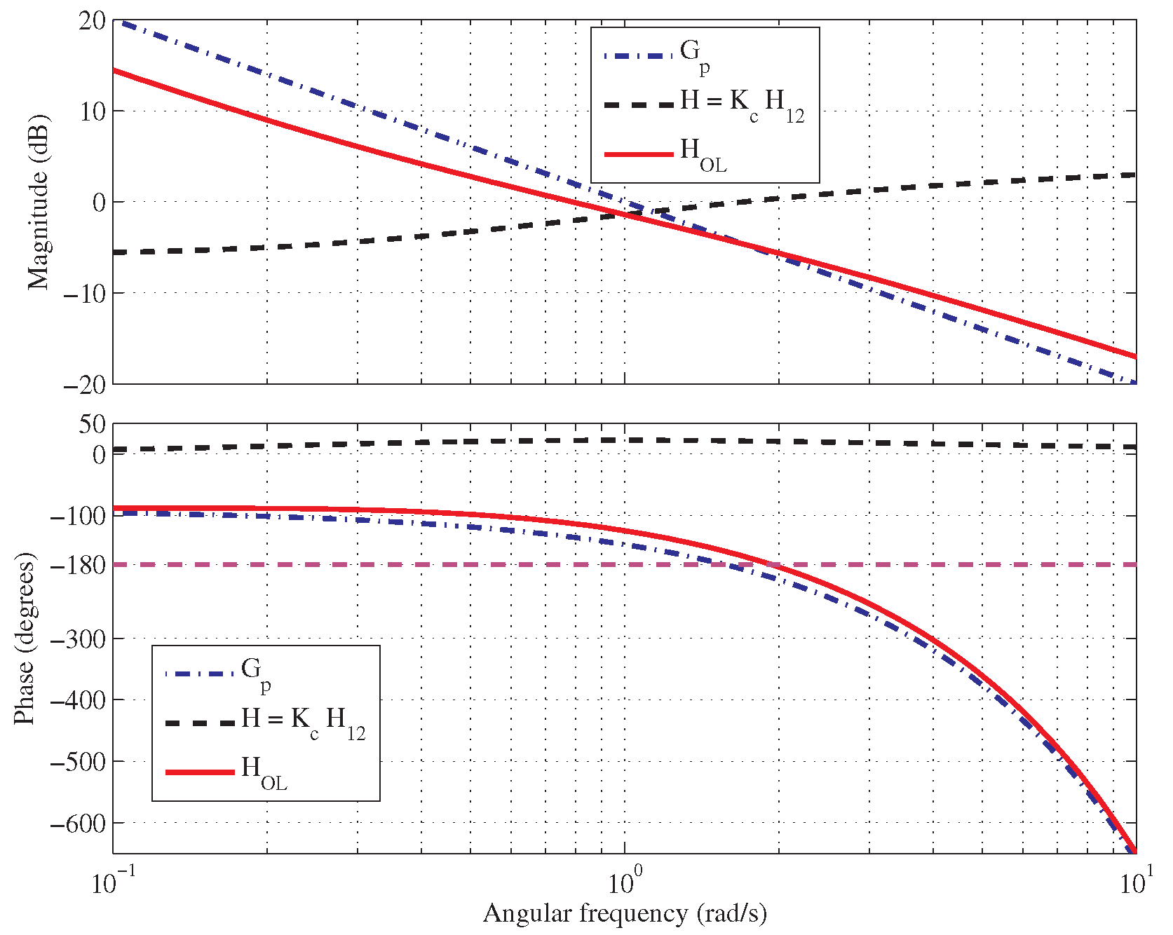
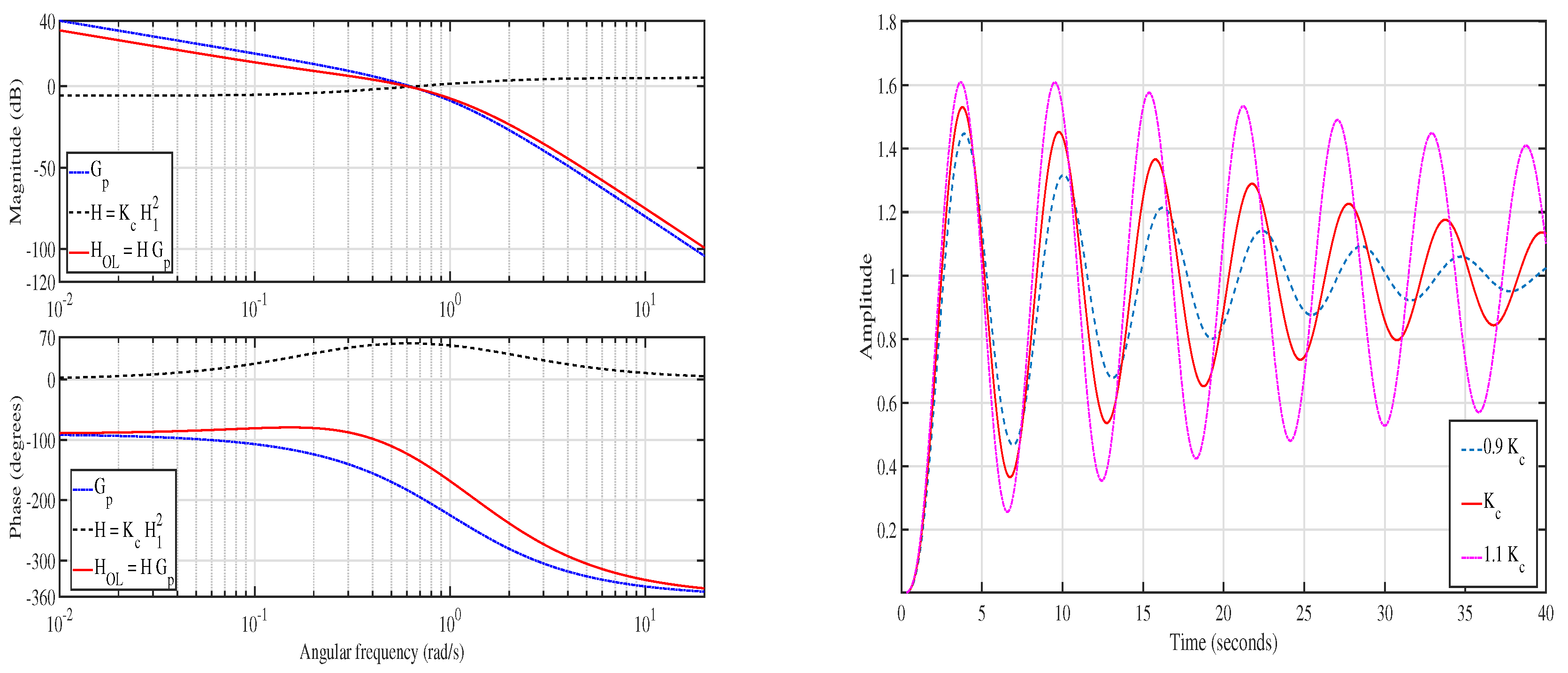
Figure 14 shows the frequency response. Although the specification on phase margin is met and the crossover is kept the same, the phase diagram is not as flat as with a CS-FLEC. Namely, the slope in the crossover is , which is only a bit lower than before compensation. Moreover, as shown by the same Figure 14, the step response shows a overshoot, sustained oscillations, a long settling time. Finally, variations with the gain are much more significant than with a CS-FLEC: with a 10% gain reduction, the overshoot is 44.7%, while with a 10% gain increase, the overshoot is 60.9%. All of these considerations explain why the CS-FLEC is preferable to a conventional cascade of identical FLECs.
5.2. Second Example
Whenever it does not compromise the clarity, the same symbols are used as the notations of the first case-study. Consider a plant that consists of an integrator with a time delay D:
that is another common reference model. This case-study has also been considered by [49]. Moreover, time-delays are important in modeling many physical devices, such as large-scale flexible structures or electric networks [73]. For this reason, the results shown here were obtained by simulating (21) without approximating the dead-time element.
For instance, if s, Figure 8 shows the Bode diagrams of with rad/s, then and . After few iterations of the step-wise algorithm, the proposed design pattern, with and with the specification , gives: s; and ; ; a phase margin of in rad/s. Moreover, . The controller is realized by
Figure 8 shows the frequency response of the compensated system and Figure 15 illustrates the step response, whose characteristics are presented in Table 1. The step response shows a overshoot and settling time of s with the designed parameters. However, variations of the gain induce and s. If changes, and s. Similar considerations to the first case hold for the control variable and the disturbance rejection.
Note that some rules can be established to guide the controller design.
- (a)
- The initial choice in the design procedure, and , is sufficient for small delays .
- (b)
- The positions and are applied to delays .
- (c)
- The design choice and can be used to satisfy the specifications and obtain good performance for delays (see Table 2).
- (d)
- The relations and are used for delays that are more difficult to compensate.
Subsequently, these rules may help the control engineer and set the limits of application of the proposed controllers.
6. Conclusions
The introduced CS-FLEC are new types of two-stages fractional-order controllers, whose phase diagrams are nearly flat in large frequency intervals of the Bode plots. Each stage of the cascade can be implemented as a second-order TF, which approximates irrational FLEC elements with sufficient accuracy. Because it is composed by a series of independent stages, a CS-FLEC is approximated by cascade of rational low-order TFs with limited coefficients sensitivity to parameter variations. Different alternatives in choosing the number of stages and their free parameters make these new controllers flexible and suitable for also solving difficult control problems. The potentiality of the CS-FLEC has been tested for controlling two plants that often are assumed as benchmark to verify the design proposals. The introduced design method follows an intuitive, practical pattern based on the developed formulas. Namely, the main strategy consists in compensating the rapidly and monotonically increasing phase lag by the lead introduced by the CS-FLEC in the same frequency range. The two examples show that the CS-FLEC allows for a desired set-point response and the stability robustness to gain and parameter variations. Finally, the study of the second benchmark identifies the interval values of the dead-time D, where the CS-FLEC can be used to satisfy strict specifications.
Funding
This research received no external funding.
Conflicts of Interest
The author declares no conflict of interest.
Abbreviations
The following abbreviations are used in this manuscript:
| PID | Proportional-Integral-Derivative |
| FOC | Fractional-Order Controller |
| FPID | Fractional-Order PID |
| FPI | Fractional-Order PI |
| PSO | Particle Swarm Optimization |
| ITAE | Integral Time Absolute Error |
| ISE | Integral Square Error |
| IAE | Integral Absolute Error |
| FLEC | Fractional-Order Lead Compensator |
| CS-FLEC | Cascaded Shifted Fractional-Order Lead Compensator |
| TF | Transfer Function |
| PM | Phase Margin |
Appendix A. The Approximation Method
The realization of the FLEC is based on a rational second-order TF approximation of the basic function :
The coefficients , depend on and can be obtained by the general approach proposed in [71]. Then the variable transformation
converts Equation (A1) in the rational TF approximating the FLEC. Namely, substituting Equation (A2) in (A1) gives:
Now let and indicate the Binomial Coefficients (BCs for brevity). By the Binomial Theorem and by the distributive law of the product of sums, it is easy to verify that
Appendix B. Computation of Slopes in the Bode Phase Diagrams
Here a new closed-formula is provided to analytically compute the slope of the Bode phase plot. If the open-loop TF including the CS-FLEC is
and if and , then it easily follows
that can be computed for . Then applying the chain rule for derivatives yields Equation (18).
References
- Oldham, K.B.; Spanier, J. The Fractional Calculus: Integrations and Differentiations of Arbitrary Order; Academic Press: New York, NY, USA, 1974. [Google Scholar]
- Samko, S.; Kilbas, A.; Marichev, O. Fractional Integrals and Derivatives: Theory and Applications; Cambridge University Press: Cambridge, UK, 1993. [Google Scholar]
- Miller, K.S.; Ross, B. An Introduction to the Fractional Calculus and Fractional Differential Equations; John Wiley & Sons, Inc.: New York, NY, USA, 1993. [Google Scholar]
- Kiryakova, V.S. Generalized Fractional Calculus and Applications; Longman Scientific & Technical: Harlow, UK, 1994. [Google Scholar]
- Podlubny, I. Fractional Differential Equations—An Introduction to Fractional Derivatives, Fractional Differential Equations, to Methods of Their Solution and Some of Their Applications; Academic Press: San Diego, CA, USA, 1999. [Google Scholar]
- Magin, R.L. Fractional Calculus in Bioengineering; Begell House Publishers: Redding, CT, USA, 2006. [Google Scholar]
- Tarasov, V.E. Fractional Dynamics: Applications of Fractional Calculus to Dynamics of Particles, Fields and Media; Springer: Berlin/Heidelberg, Germany, 2010. [Google Scholar]
- Uchaikin, V.E. Fractional Derivatives for Physicists and Engineers: Background and Theory; Springer: Berlin/Heidelberg, Germany, 2013. [Google Scholar]
- Sapuppo, F.; Bucolo, M.; Intaglietta, M.; Fortuna, L.; Arena, P. A cellular nonlinear network: Real-time technology for the analysis of microfluidic phenomena in blood vessels. Nanotechnology 2006, 17, S54–S63. [Google Scholar]
- Cairone, F.; Gagliano, S.; Bucolo, M. Experimental study on the slug flow in a serpentine microchannel. Exp. Therm. Fluid Sci. 2016, 76, 34–44. [Google Scholar]
- Lino, P.; Maione, G.; Saponaro, F. Fractional-order modeling of high-pressure fluid-dynamic flows: An automotive application. In Proceedings of the 8th Vienna International Conference on Mathematical Modelling, Vienna, Austria, 18–20 February 2013; IFAC-PapersOnLine. Volume 8, Part 1. pp. 382–387. [Google Scholar]
- Garrappa, R.; Lino, P.; Maione, G.; Saponaro, F. Model optimization and flow rate prediction in electro-injectors of Diesel injection systems. In Proceedings of the 8th IFAC International Symposium on Advances in Automotive Control (AAC 2016), Norrköping, Sweden, 19–23 June 2016; IFAC-PapersOnLine. Volume 49, pp. 484–489. [Google Scholar]
- Kapetina, M.N.; Lino, P.; Maione, G.; Rapaić, M.R. Estimation of non-integer order models to represent the pressure dynamics in common-rail natural gas engines. In Proceedings of the 20th IFAC World Congress, Toulouse, France, 9–14 July 2017; IFAC-PapersOnLine. Volume 50, pp. 14551–14556. [Google Scholar]
- Åström, K.J.; Hägglund, T. PID Controllers: Theory, Design, and Tuning, 2nd ed.; Instrument Society of America: Research Triangle Park, NC, USA, 1995. [Google Scholar]
- Oustaloup, A. La Commande CRONE. Commande Robuste d’Ordre Non Entiér; Hermés: Paris, France, 1991. [Google Scholar]
- Chen, Y.Q. Ubiquitous fractional order controls? In Proceedings of the Second IFAC Symposium on Fractional Derivatives and Its Applications (IFAC FDA06), Porto, Portugal, 19–21 July 2006; pp. 481–492. [Google Scholar]
- Monje, C.A.; Vinagre, B.M.; Feliu, V.; Chen, Y.Q. Tuning and auto-tuning of fractional order controllers for industry applications. Control Eng. Pract. 2008, 16, 798–812. [Google Scholar]
- Monje, C.A.; Chen, Y.Q.; Vinagre, B.M.; Xue, D.; Feliu, V. Fractional Order Systems and Controls. Fundamentals and Applications; Springer: London, UK, 2010. [Google Scholar]
- Efe, M.O. Fractional order systems in industrial automation. A survey. IEEE Trans. Ind. Inform. 2011, 7, 582–591. [Google Scholar]
- Caponetto, R.; Dongola, G.; Pappalardo, F.; Tomasello, V. Auto-tuning and fractional order controller implementation on hardware in the loop system. J. Optim. Theory Appl. 2013, 156, 141–152. [Google Scholar]
- Caponetto, R.; Maione, G.; Pisano, A.; Rapaić, M.R.; Usai, E. Analysis and shaping of the self-sustained oscillations in relay controlled fractional-order systems. Fract. Calc. Appl. Anal. 2013, 16, 93–108. [Google Scholar]
- Caponetto, R.; Dongola, G. A numerical approach for computing stability region of FO-PID controller. J. Frankl. Inst. 2013, 350, 871–889. [Google Scholar]
- Xue, D.; Chen, Y.Q. A comparative introduction of four fractional order controllers. In Proceedings of the 4th World Congress on Intelligent Control and Automation, Shanghai, China, 10–14 June 2002; pp. 3228–3235. [Google Scholar]
- Lurie, B.J. Three-Parameter Tunable Tilt-Integral-Derivative (TID) Controller. U.S. Patent 5371670, 6 December 1994. [Google Scholar]
- Oustaloup, A.; Mathieu, B.; Lanusse, P. The CRONE control of resonant plants: Application to a flexible transmission. Eur. J. Control 1995, 1, 113–121. [Google Scholar]
- Oustaloup, A.; Moreau, X.; Nouillant, M. The CRONE suspension. Control Eng. Pract. 1996, 4, 1101–1108. [Google Scholar]
- Podlubny, I. Fractional-order systems and PIλDμ-controllers. IEEE Trans. Autom. Control 1999, 44, 208–214. [Google Scholar]
- Raynaud, H.F.; Zergainoh, A. State-space representation for fractional order controllers. Automatica 2000, 36, 1017–1021. [Google Scholar]
- Chen, Y.Q.; Bhaskaran, T.; Xue, D. Practical tuning rules development for fractional order proportional and integral controllers. ASME J. Comput. Nonlinear Dyn. 2008, 3, 1–8. [Google Scholar]
- Barbosa, R.S.; Tenreiro Machado, J.A.; Ferreira, I. Tuning PID controllers based on Bode’s ideal transfer function. Nonlinear Dyn. 2004, 38, 305–321. [Google Scholar]
- Maiti, D.; Acharya, A.; Chakraborty, M.; Konar, A.; Janarthanan, R. Tuning PID and PIλDδ controllers using the integral time absolute error criterion. In Proceedings of the 4th International Conference on Information and Automation for Sustainability, Colombo, Sri Lanka, 12–14 December 2008; pp. 457–462. [Google Scholar]
- Chang, F.K.; Lee, C.H. Design of fractional PID control via hybrid of electromagnetism-like and genetic algorithms. In Proceedings of the Eighth International Conference on Intelligent Systems Design and Applications, Kaohsiung, Taiwan, 26–28 November 2008; pp. 525–530. [Google Scholar]
- Cao, J.Y.; Liang, J.; Cao, B.G. Optimization of fractional order PID based on genetic algorithms. In Proceedings of the Fourth International Conference on Machine Learning and Cybernetics, Guangzhou, China, 18–21 August 2005; pp. 5686–5689. [Google Scholar]
- Boškovic, M.; Rapaić, M.; Jeličić, Z. Particle swarm optimization of PID controller under constraints on performance and robustness. Int. J. Electr. Eng. Comput. 2018, 2, 1–10. [Google Scholar]
- Jakovljević, B.B.; Rapaić, M.R.; Jeličić, Z.D.; Šekara, T.B. Optimization of fractional PID controller by maximization of the criterion that combines the integral gain and closed-loop system bandwidth. In Proceedings of the 2014 18th International Conference on System Theory, Control and Computing (ICSTCC), Sinaia, Romania, 17–19 October 2014; pp. 64–69. [Google Scholar]
- Maione, G.; Punzi, A. Combining differential evolution and particle swarm optimization to tune and realize fractional order controllers. Math. Comput. Model. Dyn. Syst. 2013, 19, 277–299. [Google Scholar]
- Barbosa, R.S.; Tenreiro Machado, J.A.; Jesus, I.S. On the fractional PID control of a laboratory servo system. In Proceedings of the 17th IFAC World Congress, Seoul, Korea, 6–11 July 2008; pp. 15273–15278. [Google Scholar]
- Valerio, D.; Sá da Costa, J. Tuning of fractional PID controllers with Ziegler—Nichols-type rules. Signal Process. 2010, 86, 2771–2784. [Google Scholar]
- Maione, G.; Lino, P. New tuning rules for fractional PIα controllers. Nonlinear Dyn. 2007, 49, 251–257. [Google Scholar]
- Monje, C.A.; Calderon, A.J.; Vinagre, B.M.; Chen, Y.Q.; Feliu, V. On fractional PIλ controllers: Some tuning rules for robustness to plant uncertainties. Nonlinear Dyn. 2004, 38, 369–381. [Google Scholar]
- Luo, Y.; Chen, Y.Q.; Wang, C.Y.; Pi, Y.G. Tuning fractional order proportional integral controllers for fractional order systems. J. Process. Control 2010, 20, 823–831. [Google Scholar]
- Chen, Y.Q.; Moore, K.L.; Vinagre, B.M.; Podlubny, I. Robust PID controller autotuning with a phase shaper. In Proceedings of the First IFAC Workshop on Fractional Differentiation and Its Application (ENSEIRB), Bordeaux, France, 19–21 July 2004; pp. 162–167. [Google Scholar]
- Chen, Y.Q.; Moore, K.L. Relay feedback tuning of robust PID controllers with iso-damping property. IEEE Trans. Syst. Man Cybern. Part B Cybern. 2005, 35, 23–31. [Google Scholar]
- Monje, C.A.; Vinagre, B.M.; Chen, Y.Q.; Feliu, V.; Lanusse, P.; Sabatier, J. Proposals for fractional PIλDμ tuning. In Proceedings of the First IFAC Symposium on Fractional Differentiation and Its Application (FDA04), Bordeaux, France, 19–21 July 2004; pp. 115–120. [Google Scholar]
- Das, S.; Saha, S.; Das, S.; Gupta, A. On the selection of tuning methodology of FOPID controllers for the control of higher order processes. ISA Trans. 2011, 50, 376–388. [Google Scholar]
- Tavakoli-Kakhki, M.; Haeri, M. Fractional order model reduction approach based on retention the dominant dynamics: Application in IMC based tuning of FOPI and FOPID controllers. ISA Trans. 2011, 50, 431–441. [Google Scholar]
- Zhang, B.T.; Pi, Y.G.; Luo, Y. Fractional order sliding-mode control based on parameters auto-tuning for velocity control of permanent magnet synchronous motor. ISA Trans. 2012, 51, 649–656. [Google Scholar]
- Tavazoei, M.S.; Tavakoli-Kakhki, M. Compensation by fractional-order phase-lead/lag compensators. IET Control Theory Appl. 2014, 8, 319–329. [Google Scholar]
- Åström, K.J.; Panagopoulos, H.; Hägglund, T. Design of PI controllers based on non-convex optimization. Automatica 1998, 34, 585–601. [Google Scholar]
- Panagopoulos, H.; Åström, K.J.; Hägglund, T. Design of PID controllers based on constrained optimization. IEE Proc. Control Theory Appl. 2002, 149, 32–40. [Google Scholar]
- Monje, C.A.; Calderon, A.J.; Vinagre, B.M.; Feliu, V. The fractional order lead compensator. In Proceedings of the 2nd International Conference on Computational Cybernetics (ICCC 2004), Vienna, Austria, 30 August–1 September 2004; pp. 347–352. [Google Scholar]
- Seborg, D.E.; Edgar, T.F.; Mellichamp, D.A. Process Dynamics and Control, 2nd ed.; John Wiley & Sons, Inc.: New York, NY, USA, 2004. [Google Scholar]
- Carlson, G.E.; Halijak, C.A. Approximation of fractional capacitors (1/s)1/n by a regular Newton process. IEEE Trans. Circuit Theory 1964, 11, 210–213. [Google Scholar]
- Charef, A.; Sun, H.H.; Tsao, Y.Y.; Onaral, B. Fractal system as represented by singularity function. IEEE Trans. Autom. Control 1992, 37, 1465–1470. [Google Scholar]
- Matsuda, K.; Fujii, H. H∞ optimized wave-absorbing control: Analytical and experimental results. J. Guid. Control Dyn. 1993, 16, 1146–1153. [Google Scholar]
- Oustaloup, A.; Levron, F.; Mathieu, B.; Nanot, F.M. Frequency-band complex noninteger differentiator: Characterization and synthesis. IEEE Trans. Circuits Syst. Fundam. Theory Appl. 2000, 47, 25–39. [Google Scholar]
- Xue, D.; Zhao, C.; Chen, Y.Q. A modified approximation method of fractional order system. In Proceedings of the IEEE International Conference on Mechatronics and Automation, Luoyang, China, 25–28 June 2006; pp. 1043–1048. [Google Scholar]
- Vinagre, B.M.; Podlubny, I.; Hernández, A.; Feliu, V. Some approximations of fractional order operators used in control theory and applications. Fract. Calc. Appl. Anal. 2000, 3, 231–248. [Google Scholar]
- Podlubny, I.; Petráš, I.; Vinagre, B.M.; O’Leary, P.; Dorčák, L. Analogue realizations of fractional-order controllers. Nonlinear Dyn. 2002, 29, 281–296. [Google Scholar]
- Valério, D. Fractional Robust System Control. Ph.D. Thesis, Instituto Superior Técnico, Universidade Técnica de Lisboa, Lisbon, Portugal, 2005. [Google Scholar]
- Muñiz-Montero, C.; Sánchez-Gaspariano, L.A.; Sánchez-López, C.; González-Díaz, V.R.; Tlelo-Cuautle, E. On the electronic realizations of fractional-order phase-lead-lag compensators with OpAmps and FPAAs. In Fractional Order Control and Synchronization of Chaotic Systems, Studies in Computational Intelligence; Azar, A., Vaidyanathan, S., Ouannas, A., Eds.; Springer: Cham, Switzerland, 2017; Volume 688, pp. 131–164. [Google Scholar]
- Jadhav, S.P.; Chile, R.H.; Hamde, S.T. A simple method to design robust fractional-order lead compensator. Int. J. Control Autom. Syst. 2017, 15, 1236–1248. [Google Scholar]
- Yuan, J.; Zhenlong, W.; Shumin, F.; Chen, Y.Q. Hybrid model-based feedforward and fractional-order feedback control design for the benchmark refrigeration system. Ind. Eng. Chem. Res. 2019, 58, 17885–17897. [Google Scholar]
- Ozdemir, A.A.; Gumussoy, S. Transfer function estimation in system identification toolbox via vector fitting. IFAC-PapersOnLine 2017, 50, 6232–6237. [Google Scholar]
- Bingi, K.; Ibrahim, R.; Karsiti, M.N.; Hassam, S.M.; Harindran, V.R. Frequency response based curve fitting approximation of fractional-order PID controllers. Int. J. Appl. Math. Comput. Sci. 2019, 29, 311–326. [Google Scholar]
- Bingi, K.; Ibrahim, R.; Karsiti, M.N.; Hassan, S.M.; Harindran, V.R. Fractional-order Systems and PID Controllers—Using Scilab and Curve Fitting Based Approximation Techniques; Springer: Cham, Switzerland, 2020. [Google Scholar]
- Kapoulea, S.; Tsirimokou, G.; Psychalinos, C.; Elwakil, A.S. Employment of the Padé approximation for implementing fractional-order lead/lag compensators. AEU Int. J. Electron. Commun. 2020, 120, 153203. [Google Scholar]
- Bošković, M.Č.; Rapaić, M.R.; Šekara, T.B.; Mandić, P.D.; Lazarević, M.P.; Cvetković, B.; Lutovac, B.; Daković, M. On the rational representation of fractional order lead compensator using pade approximation. In Proceedings of the 2018 7th Mediterranean Conference on Embedded Computing (MECO), Budva, Montenegro, 10–14 June 2018; pp. 1–4. [Google Scholar]
- Maione, G. High-speed digital realizations of fractional operators in the delta domain. IEEE Trans. Autom. Control 2011, 56, 697–702. [Google Scholar]
- Caponetto, R.; Tomasello, V.; Lino, P.; Maione, G. Design and efficient implementation of digital non-integer order controllers for electro-mechanical systems. J. Vib. Control 2016, 22, 2196–2210. [Google Scholar]
- Maione, G. Continued fractions approximation of the impulse response of fractional order dynamic systems. IET Control Theory Appl. 2008, 2, 564–572. [Google Scholar]
- Middleton, R.H. Dealing with actuator saturation. In The Control Handbook; Levine, W.S., Ed.; CRC Press: Boca Raton, FL, USA, 1996; pp. 377–381. [Google Scholar]
- Bucolo, M.; Buscarino, A.; Fortuna, L.; Frasca, M. Forward action to make time-delay systems positive-real or negative-imaginary. Syst. Control Lett. 2019, 131, 104495. [Google Scholar]
Figure 1.
Bode magnitude diagrams of the FLECs (solid lines) and of the second-order realizations (dashed lines) for .
Figure 1.
Bode magnitude diagrams of the FLECs (solid lines) and of the second-order realizations (dashed lines) for .

Figure 2.
Bode phase diagrams of the FLECs (solid lines) and of the second-order realizations (dashed lines) for .
Figure 2.
Bode phase diagrams of the FLECs (solid lines) and of the second-order realizations (dashed lines) for .

Figure 3.
Bode magnitude diagrams of (dashed lines), (dash-dotted lines) and (solid lines) for 0.7 (curves ).
Figure 3.
Bode magnitude diagrams of (dashed lines), (dash-dotted lines) and (solid lines) for 0.7 (curves ).

Figure 4.
Bode phase diagrams of (dashed lines), (dash-dotted lines) and (solid lines) for 0.7 (curves ).
Figure 4.
Bode phase diagrams of (dashed lines), (dash-dotted lines) and (solid lines) for 0.7 (curves ).

Figure 5.
Bode magnitude diagrams of (dashed lines) and of the Cascaded, Shifted, Fractional-order, LEad Compensators (CS-FLEC) (solid lines) for .
Figure 5.
Bode magnitude diagrams of (dashed lines) and of the Cascaded, Shifted, Fractional-order, LEad Compensators (CS-FLEC) (solid lines) for .

Figure 6.
Bode phase diagrams of (dashed lines) and of the CS-FLEC (solid lines) for .

Figure 7.
Frequency response by the first plant (dash-dotted lines), the compensator H with the CS-FLEC (dashed lines) and the compensated system (solid lines).
Figure 7.
Frequency response by the first plant (dash-dotted lines), the compensator H with the CS-FLEC (dashed lines) and the compensated system (solid lines).

Figure 8.
Frequency response by the second plant (dash-dotted lines), the compensator H with the CS-FLEC (dashed lines) and the compensated system (solid lines).
Figure 8.
Frequency response by the second plant (dash-dotted lines), the compensator H with the CS-FLEC (dashed lines) and the compensated system (solid lines).

Figure 9.
Unit step response in the first example for different values of .

Figure 10.
Unit step response in the first example for different plant time constants.

Figure 11.
Unit step response in the first example for different fractional orders.

Figure 12.
Control variable in the first example for different values of .

Figure 13.
Step disturbance rejection in the first example for different values of .

Figure 14.
Left: frequency response by the first plant (dash-dotted lines), the compensator H with two identical FLECs (dashed lines), and the compensated system (solid lines). Right: unit step response for different values of .
Figure 14.
Left: frequency response by the first plant (dash-dotted lines), the compensator H with two identical FLECs (dashed lines), and the compensated system (solid lines). Right: unit step response for different values of .

Figure 15.
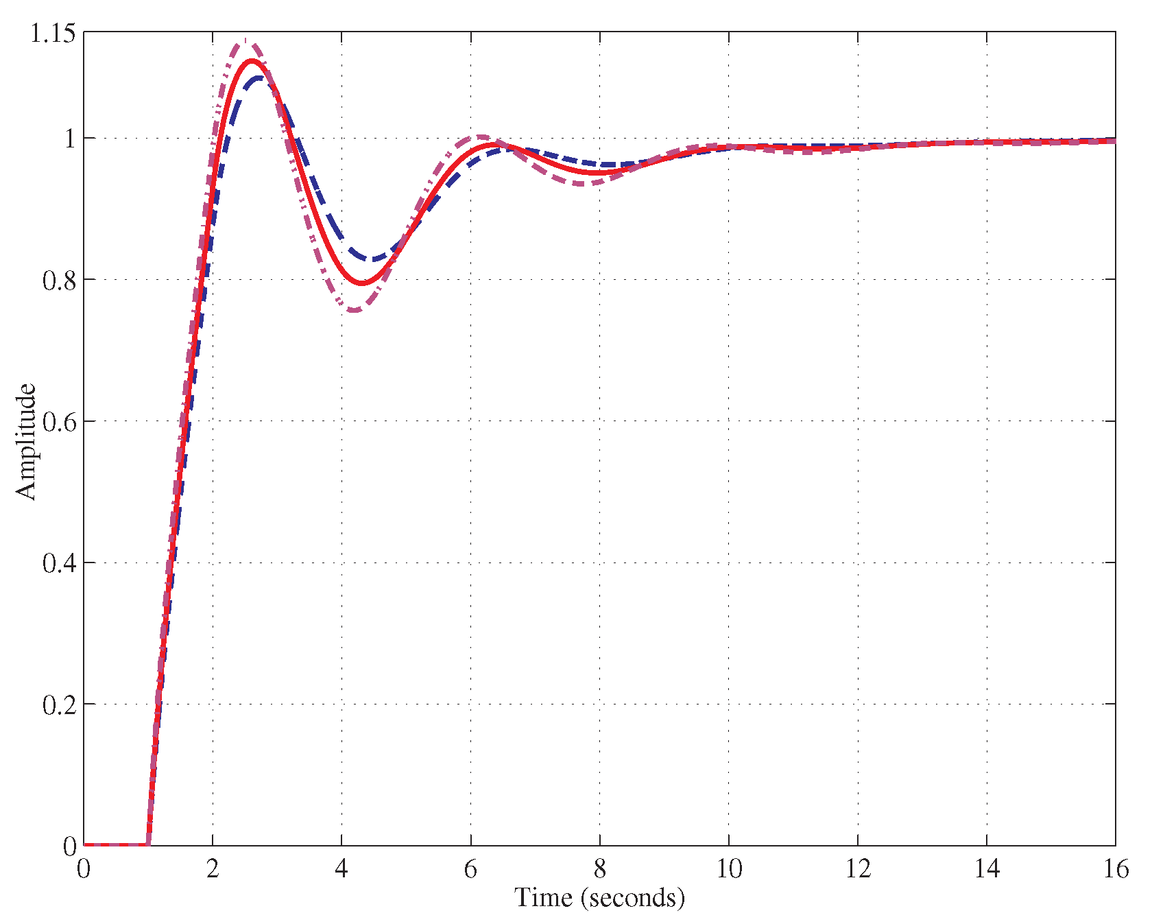
Unit step response in the second example for different fractional orders.


Table 1.
Characteristics of the step response with parameter variations: , (expressed in seconds), (in % values). Changing parameters: , , . Design values: , , (first example); , , (second example).
Table 1.
Characteristics of the step response with parameter variations: , (expressed in seconds), (in % values). Changing parameters: , , . Design values: , , (first example); , , (second example).
| First example | 0.9 | 2.46 | 0.90 | 21.47 | ||
| 2.19 | 6.55 | 18.50 | ||||
| 1.1 | 2.00 | 11.90 | 17.34 | |||
| 0.9 | 2.04 | 4.46 | 21.30 | |||
| 1.1 | 2.34 | 8.64 | 19.29 | |||
| 0.9 | 2.38 | 6.68 | 19.01 | |||
| 1.1 | 2.01 | 6.70 | 21.90 | |||
| Second example | 0.9 | – | 1.03 | 2.16 | 10.30 | |
| – | 0.89 | 10.89 | 9.40 | |||
| 1.1 | – | 0.78 | 19.71 | 9.03 | ||
| – | 0.9 | 0.95 | 8.47 | 9.56 | ||
| – | 1.1 | 0.82 | 13.76 | 11.47 |
Table 2.
Characteristics of the step response for with parameter variations: , (expressed in seconds), (in % values). Changing parameters: , .
Table 2.
Characteristics of the step response for with parameter variations: , (expressed in seconds), (in % values). Changing parameters: , .
| 0.9 | 1.01 | 3.01 | 12.95 | ||
| 0.87 | 12.65 | 12.65 | |||
| 1.1 | 0.76 | 22.38 | 12.58 | ||
| 0.9 | 0.96 | 8.87 | 10.15 | ||
| 1.1 | 0.78 | 17.24 | 12.50 | ||
| 0.9 | 1.00 | 4.04 | 14.12 | ||
| 0.85 | 14.54 | 13.32 | |||
| 1.1 | 0.73 | 25.12 | 16.29 | ||
| 0.9 | 0.96 | 9.05 | 13.60 | ||
| 1.1 | 0.74 | 21.23 | 16.06 |
© 2020 by the author. Licensee MDPI, Basel, Switzerland. This article is an open access article distributed under the terms and conditions of the Creative Commons Attribution (CC BY) license (http://creativecommons.org/licenses/by/4.0/).
Share and Cite
MDPI and ACS Style
Maione, G. Design of Cascaded and Shifted Fractional-Order Lead Compensators for Plants with Monotonically Increasing Lags. Fractal Fract. 2020, 4, 37. https://0-doi-org.brum.beds.ac.uk/10.3390/fractalfract4030037
AMA Style
Maione G. Design of Cascaded and Shifted Fractional-Order Lead Compensators for Plants with Monotonically Increasing Lags. Fractal and Fractional. 2020; 4(3):37. https://0-doi-org.brum.beds.ac.uk/10.3390/fractalfract4030037
Chicago/Turabian StyleMaione, Guido. 2020. "Design of Cascaded and Shifted Fractional-Order Lead Compensators for Plants with Monotonically Increasing Lags" Fractal and Fractional 4, no. 3: 37. https://0-doi-org.brum.beds.ac.uk/10.3390/fractalfract4030037