Fractional SIS Epidemic Models


Department of Basic and Applied Sciences for Engineering, Sapienza University of Rome, 00161 Rome, Italy
*
Author to whom correspondence should be addressed.
†
These authors contributed equally to this work.
Fractal Fract. 2020, 4(3), 44; https://0-doi-org.brum.beds.ac.uk/10.3390/fractalfract4030044
Submission received: 22 July 2020
/
Revised: 24 August 2020
/
Accepted: 28 August 2020
/
Published: 31 August 2020
(This article belongs to the Special Issue Fractional Behavior in Nature 2019)
Abstract
:In this paper, we consider the fractional SIS (susceptible-infectious-susceptible) epidemic model (α-SIS model) in the case of constant population size. We provide a representation of the explicit solution to the fractional model and we illustrate the results by numerical schemes. A comparison with the limit case when the fractional order α converges to 1 (the SIS model) is also given. We analyze the effects of the fractional derivatives by comparing the SIS and the α-SIS models.
1. Introduction
The study of mathematical models for epidemiology has a long history, dating back to the early 1900s with the theory developed by Kermack and McKendrick [1]. Such theory describes compartmental models, where the population is divided into groups depending on the state of individuals with respect to disease, distinguishing between groups. The dynamic of the disease is then described by a system of ordinary differential equations for each class of individuals. The use of mathematical models for epidemiology is particularly useful to predict the progress of an infection and to take strategy to limit the spread of the disease. In this work, we focus on the α-SIS (susceptible-infectious-susceptible) epidemiological model. The SIS model has a long history, too [2]. It describes the spread of human viruses, such as influenza. The SIS model with constant population is particularly appropriate to describe some bacterial agent diseases, such as gonorrhea, meningitis, and streptococcal sore throat. SIS is a model without immunity, where the individual recovered from the infection comes back into the class of susceptibles.
1.1. Statement of the Problem
We propose an α-SIS model with constant population size. The novelty concerns the SIS equations with the time fractional Caputo derivative in place of time standard derivative and their explicit solutions in terms of Euler’s numbers and Euler’s Gamma functions.
Let us consider the Caputo fractional derivative introduced in (Section 2.1) below. We provide an explicit representation of the solution to
for the constant population case , , where is the order of the Caputo fractional derivative, is the birth rate and the death removal rate, is the contact rate, and is the recovery removal rate. The unknown functions and represent the percentage of susceptible and infected people at time with initial data and . As far as we know, although, in the numerical literature, it is an unknown formula for the solution. By using a series representation for the solution to the fractional logistic equation we may give an explicit formula for the unknown functions S and I. From the numerical point of view, we validate the goodness of the theoretical formulas by applying two different numerical schemes. Then, we compare the fractional case results () with the well-known standard case taking the limit converges to 1, and we analyze the effects produced by the fractional derivatives.
1.2. Motivations
Let us consider an infective disease which does not confer immunity and which is transmitted through contact between people. We divide the population into two disjoint classes which evolve in time: the susceptibles and the infectives. The first class contains the individuals which are not yet infected but who can contract the disease; the second class contains the infected population which can transmit the disease. The SIS model [2] is a simple disease model without immunity, where the individuals recovered from the infection come back into the class of susceptibles. Such a model is used to describe the dynamic of infections which do not confer a long immunity, such as a cold or influenza. Fractional calculus is therefore considered in biological models to take into account macroscopic effect. The use of fractional derivatives in the model means that some global effect may produce slowdown in the process. This is verified and discussed in the validation of the model.
1.3. State of the Art
The logistic function was introduced by Pierre Francois Verhulst [3] to model the population growth. At the beginning of the process, the growth of the population is fast; then, as saturation process begins, the growth slows, and then growth is close to be flat. The problem to give a solution of the fractional logistic equation was unsolved and several attempts have been done (see, for instance, Reference [4,5,6,7]). Concerning the fractional SIS model, some works can be listed about numerical solutions obtained by considering different methods. The existence and uniqueness of the solution have been discussed in Reference [8] in case of constant population size. Moreover, in that work, the authors have studied a numerical solution by variational iteration method and Euler method. In the previous paper of Reference [9], the case of variable population size has been considered and the stability of the equilibrium point has been investigated together with the existence of the solution. From the technical point of view our result take advantage of the explicit representation by series of the solution of fractional logistic equation solved in the recent paper of Reference [10]. Thanks to a fruitful formulation of the SIS model, we are able to adapt the results obtained for fractional logistic equation in Reference [10] and to give the solution of fractional SIS model by series. For the physical derivation of the fractional model, we refer to the interesting paper of Reference [11], in which the authors have considered a probabilistic approach in terms of continuous-time random walk in order to obtain the fractional SIR model.
In recent years, the study of epidemiological models using fractional calculus has spread widely. In Reference [12], the authors prove via numerical simulations that the proposed fractional model gives better results than the classical theory, when compared to real data. Moreover, for some diseases, it is necessary to take into account the history of the system (see, for example, Reference [13]); thus, non-locality and memory become important to model real data. Indeed, fractional operators consider the entire history of the biological process, and we are able to model non-local effects often encountered in biological phenomena.
1.4. Main Results
We provide an explicit representation of the solution to
in terms of uniformly convergent series on compact sets.
Let us introduce the basic reproduction number [14], i.e., the expected number of secondary infections produced during the period of infection, which is given by
where is the infection period. Let
be the so-called carrying capacity and define . The problem (1) can be solved by considering, for , the fractional logistic equation
In the following theorems, denotes the Beta function, denotes the Euler Gamma function, and is the -Euler’s number introduced in Reference [10].
Theorem 1.
Let , and . An explicit representation of the solution of the fractional model (1) with initial condition and is given by
with
and
The series is uniformly convergent on any compact subset , where
Theorem 2.
Let , . An explicit representation of the solution of the fractional SIS model (1) with initial condition and is given by
with and
The series converges uniformly in with .
1.5. Outline
The paper is organized as follows. In Section 2, we introduce the fractional α-SIS model with constant population size. In Section 3, we prove the main results of the paper. In Section 4, we validate the model using two numerical schemes, and we provide some numerical tests also comparing the α-SIS model with the SIS one.
2. The Settings
In this section, we briefly review the mathematical background on fractional derivatives and its connection with the SIS model.
2.1. The Fractional Derivatives
Fractional Calculus has a long history, starting from some works by Leibniz (1695) or Abel (1823), to where it has been developed up to today. The literature is vast and many definitions of fractional derivatives has been given. We recall the well-known derivatives of Caputo and Riemann-Liouville given by following the definitions we will deal with throughout. The Caputo Derivative of a function is written as
whereas the Riemann-Liouville derivative of is defined as follows:
Notice that, for , if such that and a.e. with , then we have that for
where
is the Beta function and , is the Euler’s gamma function. The Caputo and the Riemann-Liouville fractional derivatives are linked by the following formula:
which will be useful further on. We list some useful properties of the Caputo derivative:
- (P1)
- Let u be a constant function. Then .
- (P2)
- Let such that and , exist almost everywhere. Then, .
- (P3)
- Let be such that and exist almost everywhere in . Let . Then, exists almost everywhere in . In particular,
- (P4)
- Let . Then,pointwise in .
(P1) and (P3) are immediate consequences of the definition of the Caputo derivative. (P2) can be obtained from (12). (P4) follows from the definition given for . Our discussion here is based on the result in [15] (Theorem 2.20) for the Riemann-Liouville derivative and the definition (12) above of the Caputo derivative. The interested reader can also consult [16] (p. 20) in which the connection with the Marchaud derivative is considered.
Let us consider the equation on with where . Then, u is the Mittag-Leffler function
For the reader’s convenience, we write below the proof of this standard result. From the Laplace transform
where , the equation takes the form , that is
since . From the Stirling’s formula for Gamma function, we have
Thus, we get that
Thus, by the root criterion, we get an infinite radius of convergence.
2.2. The Fractional SIS Model
In the discussion above the symbols and have been used denoting percentages. Indeed, is a constant function for any t. Denoting by and the number of susceptibles and infectives, respectively, at time t, the fractional SIS model with non-constant population (see Reference [17,18] for , that is, the non-fractional case, but we say SIS model) is written as
where is the birth rate, is the death removal rate, is the contact rate, and is the recovery removal rate. The sum of susceptibles and infectives is defined by .
The problem to solve (14) is challenging for many reasons. To overcome such difficulties we introduce the difference between the susceptible and infective populations given by
from which we are able to recover the functions and as follows:
By the linearity of the Caputo derivative, (see (P3)) the problem takes the form
In this new formulation, we are able to solve (16) by using standard results.
Proposition 1.
Notice that is an increasing function as , whereas it exhibits a decreasing behavior for . Thus, we can write the non-obvious relation
We underline that the fractional derivative is a non-local operator, and we do not have a direct information about the behavior of the function under investigation.
The Equation (17) can be treated as a fractional logistic equation with a forcing term. We decided to focus on this equation in a different work. Although the problem can be studied from a numerical point of view, proceeding with a general approach seems to be hard.
Our results can be regarded as the special case , that is, constant population , . Indeed, for the Mittag-Leffler function, we have , . Thus, we turn our problem in studying the fractional logistic equation. In particular, assuming , the problem reduces to
that is, is constant and satisfies (P1), as we can see from the first equation, and the second equation is the fractional logistic equation we are interested in with the suitable characterization of all parameters. Indeed, by considering with the corresponding compartmental , , , , the equations above take the form:
and we get
where and . Remember that is a percentage; by recalling that and , we obtain
that is
from which we recover
which is (4). We notice that in this characterization the carrying capacity c merits further investigations. Indeed, it must be . We are led to study both cases and . Since, in our formulation, , we refer to and as percentages and use the symbol and .
For , the Mittag-Leffler becomes the exponential , whereas, for , we have the following asymptotic behaviors for ,
where
For , the Mittag-Leffler (18) is an increasing function.
3. Proof of the Main Results
In this section, we collect the proof of the results presented in the work. From the theory of power series, we know that to each series representation with coefficients corresponds a radius of convergence such that the series converges uniformly in for every . By the root test, we also have that
and the radius obviously depends on the sequence and the order of the fractional derivative.
Proof of Theorem 1.
Similarly to the classical case, by the linearity (P3) of the Caputo derivative, we exploit to reduce problem (1) to
We rewrite (24) as
where and . Equation (25) is the fractional logistic equation investigated in Reference [10], where the explicit solution is given for and as
In particular, the authors proved an estimate by below of the convergence ray . From (26), we recover , the solution of the α − SIS model.
Proof of Theorem 2.
By the linearity (P3) of the Caputo derivative and the fact that , the problem (1) reduces to
Setting , we have that
We prove that
solves (28); hence, is the solution to (27).
To this end, we compute the Riemann-Liouville fractional derivative of in (29), which is
By (12), we have
Now, we compute :
By (30) and (31), and by , we have
thus,
We use the fact that ,
From the definition above of the coefficients , we get
By iteration, we obtain that . Since , we write
We now consider the fact that
(where is the Mascheroni constant), and we get
Since
and
we get that
Thus, we get the radius of convergence
for the series
The convergence of the majorant series determines the uniform convergence in of the series we are interested in. This concludes the proof by considering .
Remark 1.
The solution in Theorem 1 has been given only for the initial datum . This is because of the representation given in Reference [10] in terms of Euler polynomials. Let us focus on the solution in Theorem 2. Taking , we see that, setting
where
we obtain . This is the solution in to
(see the proof of Theorem 3.1 in Reference [10]). In the special case , we know that
solves with . In particular, for , we obtain convergence in any compact sets for both solutions v and w. This underlines the fact that, by introducing non-locality, we may deal with solutions quite far from their non-linear analogues.
4. Numerical Comparison
In this section, we proceed with the validation of the previous results on the fractional SIS model by means of numerical approximations, and we analyze the effects of fractional derivatives by comparing the ordinary and fractional SIS model.
4.1. Numerical Approximation
The explicit solution (5)–(6) to the fractional SIS model (1) for is defined for and initial datum . The explicit solution (8)–(9) to the fractional SIS model (1) for is defined for the initial datum . In order to compute the solution to the fractional SIS model for any set of parameters and any initial datum, we propose and compare two numerical schemes to approximate (1). To this end, let us consider the following problem:
on a time interval uniformly divided into time steps of length . Our aim is to define the discrete solution for , where , and is known.
We refer to the following method as the Method 1. Following Reference [19], we observe that
thus, we rewrite (33) as
We introduce a Predictor-Evaluate-Corrector-Predictor (PECE) method [20]. Specifically, we use the implicit one-step Adams-Moulton method [21] (Chapter 11), i.e.,
where the coefficients and are defined below.
First of all, we compute the term with the one-step Adams-Bashforth method. We introduce and as a piece-wise linear function which interpolates g on the nodes , . We approximate the integral term of (34) with the product rectangle rule, i.e.,
where
In particular, for our uniform discretization of the time interval , we have
Therefore,
Now, we compute the coefficients ; thus, we approximate as
By using the product trapezoidal quadrature formula on the nodes , Equation (37) becomes
where are defined as
We observe that, from integration by parts, we have
and, therefore,
Finally, in our uniform grid, the coefficients are
Remark 2.
The numerical scheme described above works for any .
We now introduce a method to which we refer as Method 2. Let . In Reference [22], the authors give the following approximation of the Caputo derivative
with
and . The numerical scheme to solve (33) is then given by
We refer to Reference [22] for further details on the properties of the scheme.
Remark 3.
The numerical scheme above described works for , with the extreme values excluded.
To summarize, in this section, we have introduced two numerical schemes, which we denote here by and for notational convenience. The solution to the fractional SIS model (1) with the first numerical scheme (that is Method 1) is
where is defined in (35), and the solution with the second numerical scheme (that is Method 2) is
where is defined in (42) and . Note that the function in (33), used for both the numerical schemes, is defined as , while .
Remark 4.
The computational complexity is essentially due to the fact that fractional derivatives are non-local operators. In order to improve the speed of the iterative method the short memory principle of Podlubny [23] (p. 203) for Caputo derivative can be helpfully considered. However, the price for the reduced complexity is given by the loss in the order of accuracy (see, for example, Reference [24,25]).
4.2. Numerical Tests
In this section we compare the solutions to the fractional SIS model (1) computed with the explicit representation and the two numerical schemes, testing both the case and . In what follows, we denote by
- the solutions to the SIS model, our aim is to show the correspondence with the case ,
4.2.1. Test with
We start our numerical analysis with the case of carrying capacity . We fix this set of parameters: , , , , and . The initial data are and , the final time is , and the time step .
First of all, we compare the exact fractional solutions (5)–(6) and the two numerical solutions (43)–(44) and (45)–(46) for , which approximately corresponds to the classical derivative. Note that we do not use since the second numerical scheme works for , as already observed in Remark 3. In Figure 1, we show the results. As expected, the exact fractional solution and the two numerical solutions to (1) overlap the solution for .
In Figure 2 and Figure 3, we show the results obtained with and . In the first case, the two density curves are closer each other and the intersection point between them slightly moves to the right with respect to the solution shown in Figure 1. Such behavior is further emphasized by lower values of , as shown for example in Figure 3. Note that, in both cases, the three methodologies produces almost identical results.
To further investigate on the three methodologies, we compute the -norm of the difference between the exact fractional solutions (5)–(6) and the two numerical solutions (43)–(44) and (45)–(46) and between the two numerical solutions each others, as shown in Table 1. We observe that the errors range from orders of to , increasing with respect to the decrease of . This fact further certifies the similarity between the three proposed methodologies.
4.2.2. Test with
We focus now on the case of carrying capacity . We fix this set of parameters: , , , and . Moreover, the initial data are and , the final time is , and the time step .
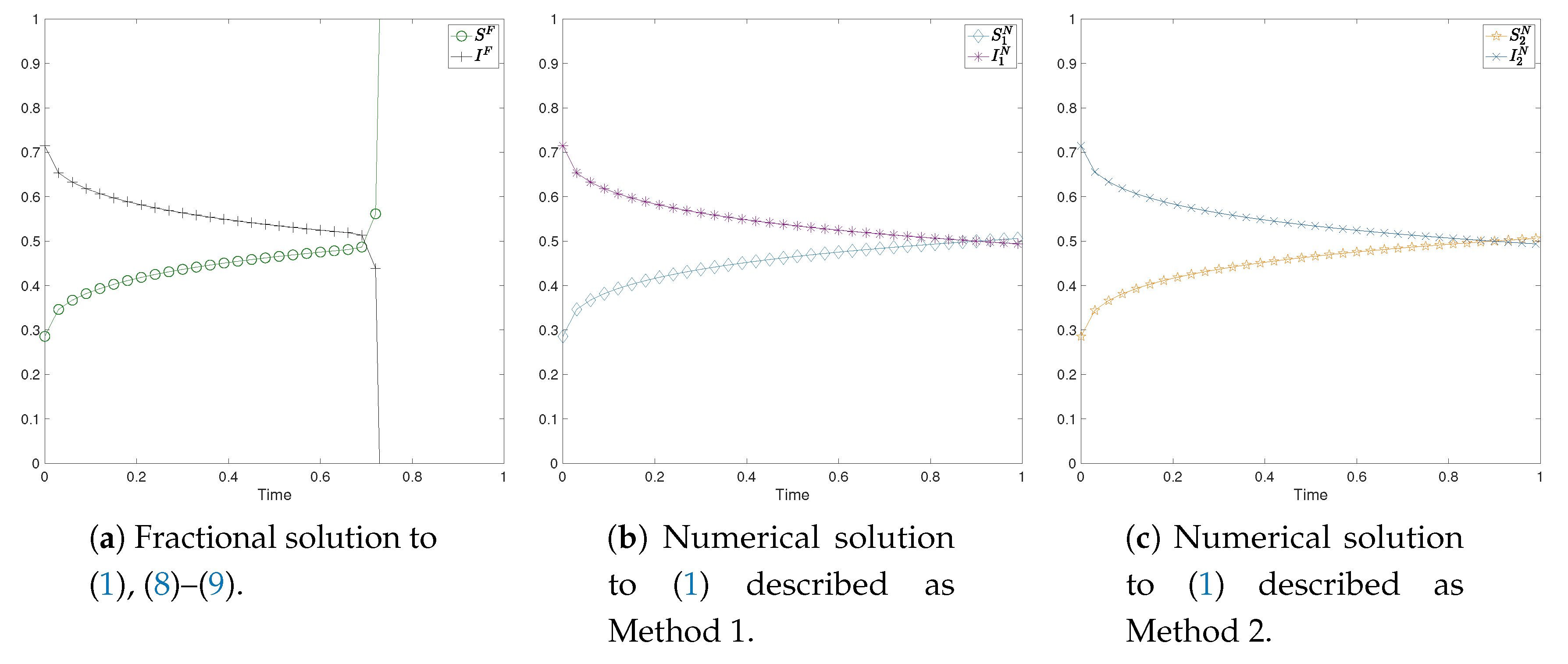
In Figure 4, we compare the exact fractional solutions (8)–(9) and the two numerical solutions (43)–(44) and (45)–(46) for . Again, we observe that the fractional solutions, both explicit and numerical, perfectly overlap the solution to the SIS model. In Figure 5, we show the results obtained with . Analogously to the example with , the point of intersection between the two densities of population slightly moves to the right with respect to the solution shown in Figure 4. Moreover, the three different methodologies produce again almost identical results. Finally, in Figure 6, we show the results obtained with . In this case, the explicit fractional solutions (8)–(9) blow up in finite time, since the final time T is greater than the radius of convergence, while the two numerical solutions show that the intersection point between the two curves further moves to the right with respect to Figure 5.
5. Conclusions
In this work, we studied the fractional SIS model with constant population size. We proposed an explicit representation of the solution to the fractional model under particular assumptions on parameters and initial data. By considering the basic reproduction number, we rearrange the SIS model and obtain a logistic equation. In the new formulation of the problem, the carrying capacity has a new meaning based on the parameters of the SIS model. We exploit such a formulation in order to study the fractional SIS model and obtain a fruitful characterization of the problem, despite many difficulties introduced by non-locality. In our formulation, the carrying capacity can equal zero, and this brings our attention to a different non-linear problem which, in turn, is related to the underlined SIS model. We introduced two different numerical schemes to approximate the model and perform numerical simulations, with which we tested the proposed explicit solution.
Author Contributions
Conceptualization; methodology; software; validation; formal analysis; investigation; writing—original draft preparation; writing—review and editing: C.B., M.D. and P.L. All authors have read and agreed to the published version of the manuscript.
Funding
The research has been done within the Ph.D. program in “Mathematical Models for Engineering, Electromagnetics and Nanosciences”, Sapienza Università di Roma.
Conflicts of Interest
The authors declare no conflict of interest. The funders had no role in the design of the study; in the collection, analyses, or interpretation of data; in the writing of the manuscript, or in the decision to publish the results.
References
- Kermack, W.O.; McKendrick, A.G. A contribution to the mathematical theory of epidemics. Proc. R. Soc. A Math. Phys. 1927, 115, 700–721. [Google Scholar]
- Hethcote, H.W. Three basic epidemiological models. In Applied Mathematical Ecology (Trieste, 1986); Springer: Berlin, Germany, 1989; Volume 18, pp. 119–144. [Google Scholar]
- Verhulst, P.F. Notice sur la loi que la population suit dans son accroissement. Corresp. Math. Phys. 1838, 10, 113–126. [Google Scholar]
- El-Sayed, A.; El-Mesiry, A.; El-Saka, H. On the fractional-order logistic equation. Appl. Math. Lett. 2007, 20, 817–823. [Google Scholar] [CrossRef] [Green Version]
- Area, I.; Losada, J.; Nieto, J.J. A note on the fractional logistic equation. Physica A 2016, 444, 182–187. [Google Scholar] [CrossRef] [Green Version]
- West, B. Exact solution to fractional logistic equation. Physica A 2015, 429, 103–108. [Google Scholar] [CrossRef]
- Yang, X.J.; Tenreiro Machado, J. A new insight into complexity from the local fractional calculus view point: Modelling growths of populations. Math. Mod. Meth. Appl. Sci. 2017, 40, 6070–6075. [Google Scholar] [CrossRef] [Green Version]
- Hassouna, M.; Ouhadan, A.; El Kinania, E. On the solution of fractional order SIS epidemic model. Chaos Solitons Fractals 2018, 117, 168–174. [Google Scholar] [CrossRef] [PubMed]
- El-Saka, H. The fractional-order SIS epidemic model with variable population size. J. Egypt. Math. Soc. 2014, 22, 50–54. [Google Scholar] [CrossRef] [Green Version]
- D’Ovidio, M.; Loreti, P. Solutions of fractional logistic equations by Euler’s numbers. Physica A 2018, 506, 1081–1092. [Google Scholar] [CrossRef] [Green Version]
- Angstmann, C.N.; Henry, B.I.; McGann, A.V. A Fractional-Order Infectivity and Recovery SIR Model. Fractal Fract. 2017, 1, 1–11. [Google Scholar]
- Pooseh, S.; Rodrigues, H.S.; Torres, D.F. Fractional derivatives in dengue epidemics. AIP Conf. Proc. 2011, 1389, 739–742. [Google Scholar] [CrossRef] [Green Version]
- Rositch, A.F.; Koshiol, J.; Hudgens, M.G.; Razzaghi, H.; Backes, D.M.; Pimenta, J.M.; Franco, E.L.; Poole, C.; Smith, J.S. Patterns of persistent genital human papillomavirus infection among women worldwide: A literature review and meta-analysis. Int. J. Cancer 2013, 133, 1271–1285. [Google Scholar] [CrossRef] [PubMed] [Green Version]
- Anderson, R.M.; May, R.M. The population dynamics of microparasites and their invertebrate hosts. Philos. Trans. R. Soc. B 1981, 291, 451–524. [Google Scholar]
- Diethelm, K. The Analysis of Fractional Differential Equations; Springer: Berlin/Heidelberg, Germany, 2010. [Google Scholar]
- Ferrari, F. Weyl and Marchaud Derivatives: A Forgotten History. Mathematics 2018, 6, 6. [Google Scholar] [CrossRef] [Green Version]
- Zhou, J.; Hethcote, H.W. Population size dependent incidence in models for diseases without immunity. J. Math. Biol. 1994, 32, 809–834. [Google Scholar] [CrossRef] [PubMed]
- Zhang, F.W.; Nie, L.F. Dynamics of SIS epidemic model with varying total population and multivaccination control strategies. Stud. Appl. Math. 2017, 139, 533–550. [Google Scholar] [CrossRef]
- Ahmed, E.; El-Sayed, A.M.A.; El-Mesiry, A.E.M.; El-Saka, H.A.A. Numerical solution for the fractional replicator equation. Int. J. Mod. Phys. C 2005, 16, 1017–1026. [Google Scholar] [CrossRef]
- Diethelm, K.; Freed, A.D. The FracPECE Subroutine for the Numerical Solution of Differential Equations of Fractional Order. Forsch. Wiss. Rechn. 1998, 1999, 57–71. [Google Scholar]
- Quarteroni, A.; Sacco, R.; Saleri, F. Numerical Mathematics, 2nd ed.; Springer: Berlin, Germany, 2007; Volume 37, p. xviii+655. [Google Scholar]
- Giga, Y.; Liu, Q.; Mitake, H. On a discrete scheme for time fractional fully nonlinear evolution equations. Asymptot. Anal. 2019, 1–12. [Google Scholar] [CrossRef] [Green Version]
- Podlubny, I. Fractional Differential Equations; Mathematics in Science and Engineering; Academic Press: Cambridge, MA, USA, 1999; Volume 198. [Google Scholar]
- Diethelm, K.; Ford, N.; Freed, A. A Predictor-Corrector Approach for the Numerical Solution of Fractional Differential Equations. Nonlinear Dyn. 1999, 29, 3–22. [Google Scholar] [CrossRef]
- Ford, N.J.; Simpson, A. The numerical solution of fractional differential equations: Speed versus accuracy. Numer. Algorithms 2001, 26, 333–346. [Google Scholar] [CrossRef]
Figure 1.
Comparison between the solutions to the susceptible-infectious-susceptible (SIS) model and the explicit and numerical fractional solutions to (1) with . The analysis shows correspondence between SIS model and the case of our model. This result was expected, and it confirms the continuity wit respect to (see (P4)).

Figure 2.
Comparison between the explicit and numerical fractional solutions to (1) with .
Figure 2.
Comparison between the explicit and numerical fractional solutions to (1) with .

Figure 3.
Comparison between the explicit and numerical fractional solutions to (1) with .
Figure 3.
Comparison between the explicit and numerical fractional solutions to (1) with .

Figure 4.
Comparison between the solutions to the SIS model and the fractional solutions to (1) with (continuity w.r. to ).
Figure 4.
Comparison between the solutions to the SIS model and the fractional solutions to (1) with (continuity w.r. to ).

Figure 5.
Comparison between the fractional solutions to (1) with .
Figure 5.
Comparison between the fractional solutions to (1) with .

Figure 6.
Comparison between the fractional solutions to (1) with .
Figure 6.
Comparison between the fractional solutions to (1) with .


Table 1.
Comparison of the -norm between the solutions computed with the three methodologies for different values of .
Table 1.
Comparison of the -norm between the solutions computed with the three methodologies for different values of .
| () | |||
|---|---|---|---|
| 0.99 | 1 × 10 | 9 × 10 | 9 × 10 |
| 0.7 | 1 × 10 | 2 × 10 | 2 × 10 |
| 0.3 | 3 × 10 | 8 × 10 | 8 × 10 |
© 2020 by the authors. Licensee MDPI, Basel, Switzerland. This article is an open access article distributed under the terms and conditions of the Creative Commons Attribution (CC BY) license (http://creativecommons.org/licenses/by/4.0/).
Share and Cite
MDPI and ACS Style
Balzotti, C.; D’Ovidio, M.; Loreti, P. Fractional SIS Epidemic Models. Fractal Fract. 2020, 4, 44. https://0-doi-org.brum.beds.ac.uk/10.3390/fractalfract4030044
AMA Style
Balzotti C, D’Ovidio M, Loreti P. Fractional SIS Epidemic Models. Fractal and Fractional. 2020; 4(3):44. https://0-doi-org.brum.beds.ac.uk/10.3390/fractalfract4030044
Chicago/Turabian StyleBalzotti, Caterina, Mirko D’Ovidio, and Paola Loreti. 2020. "Fractional SIS Epidemic Models" Fractal and Fractional 4, no. 3: 44. https://0-doi-org.brum.beds.ac.uk/10.3390/fractalfract4030044