Analysis of the Effects of the Viscous Thermal Losses in the Flute Musical Instruments

Abstract

This article presents the third part of a larger project whose final objective is to study and analyse the effects of viscous thermal losses in a flute wind musical instrument. After implementing the test bench in the first phase and modelling and validating the dynamic behaviour of the simulator, based on the previously implemented test bench (without considering the losses in the system) in the second phase, this third phase deals with the study of the viscous thermal losses that will be generated within the resonator of the flute. These losses are mainly due to the friction of the air inside the resonator with its boundaries and the changes of the temperature within this medium. They are mainly affected by the flute geometry and the materials used in the fabrication of this instrument. After modelling these losses in the frequency domain, they will be represented using a system approach where the fractional order part is separated from the system’s transfer function. Thus, this representation allows us to study, in a precise way, the influence of the fractional order behaviour on the overall system. Effectively, the fractional behavior only appears much below the 20 Hz audible frequencies, but it explains the influence of this order on the frequency response over the range [20–20,000] Hz. Some simulations will be proposed to show the effects of the fractional order on the system response.

1. Introduction

Fractional order derivative is an ancient mathematical representation that appeared in the late 16th century, and its actual implementation started fifty years ago. However, the numerical simulation of such systems is relatively new, as special tools need to be integrated in the simulators. Thus, the first efficient and inexpensive simulations introduced for simple models (conservative plane waves) were based on signal processing tools: the so-called digital waveguide formalism [1,2,3,4] and more specifically, a factored form introduced by Kelly–Lochbaum [5]. The initial idea rested on the factoring of the alembertian of the equation of plane waves into two transport operators that each govern decoupled “round trip” progressive waves, from which we could derive a form in efficient delay system for the simulation [6,7].

Furthermore, 3D and 2D models with realistic boundary conditions are far too complex to be considered, for example in real-time sound synthesis. They can be effectively reduced to a 1D wave equation including a term that models the flare of the tube profile. It is about the equation of the pavilions, which is also called model of Webster. A more elaborative version of this conservative model includes the effect of visco-thermal losses due to the boundary layers in the vicinity of the walls. This dissipative model, known as the Webster–Lokshin 1D [8,9,10], includes a term that involves a fractional derivation in time of order 3/2 [11,12,13,14,15]. This operator plays a crucial role from a perceptual point of view on sound realism [16].

Thus, the work presented in this paper is a part of a larger project. The objective is not to study the system from an acoustic musical point of view for which there are indeed many works, but from a control point of view, in particular within the framework of the dynamics of complex systems during the study of the coupling between the nonlinear exciter and the resonator (which is part of the continuity of this paper and which will be the subject of a future publication).

Concerning this work, it consists of modelling and simulating the viscous losses within the resonator of the flute musical instrument. This work is not unique, as it is a continuity of three previous publications that showed the following:

• The system consisting of the musician-flute that was implemented and modeled. It consisted of an air compressor, a servo-valve, and an artificial mouth mounted to mimic the musician’s lungs and mouth. A control system was also developed to regulate the pressure and the flow delivered to the artificial mouth. Added to that, the flute exciter was directly coupled with the artificial mouth and some pressure and temperature sensors were placed within the resonator [17,18];
• The knowledge model was developed to represent the transfer between the pressure source at the input of the tube at x = 0 and the flow at any point x of the tube of length L and of constant radius r. Partial differential equations aiming to causally decompose the global model into sub-models, and thus to facilitate analysis in the frequency domain, were used in modelling [19].

So, in more detail, the main target of this article is to analyze the effect of viscous thermal fractional order element on the sound delivered at the output of the flute. The novelty of the work resides in the numerical synthesis of the viscous thermal losses as well as in its simulation using the hardware-in-the-loop technique. This numerical simulation is important, as it allows the sweeping of the fractional order viscous thermal variable, which is mainly linked to the geometry of the flute’s resonator as well as to the materials constituting it.

This article will be divided as follows. In Section 2, the modelling of the test bench will be presented. System approach representation as well as the analysis of all the blocks will be introduced in Section 3. Section 4 presents the rationalization technique of a fractional order system in order to represent it using a series of real poles and zeros of an integer order. Finally, Section 5 summarizes this work and proposes some future tasks.

2. Modelling

2.1. Schematisation, Configuration, and Setting in Equation

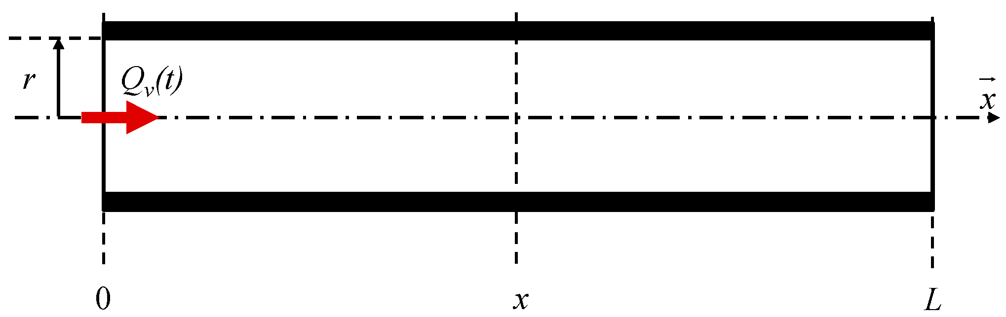
Let us consider an acoustic tube of length L and a constant radius r subjected to an acoustic flow (also called volume flow) Q_v(t) with $x=0$ where $x\in \left[0;L\right]$ (Figure 1).

When an acoustic wave propagates in the air, this sets the particles of the fluid in motion, which vibrate at a speed v(t) around their equilibrium position. Then, the acoustic flow Qv(t) measures the flow [in m³/s] of this speed through a surface and presents it as a scalar quantity [20,21,22,23,24].

The acoustic impedance Z_ac (also called specific acoustic impedance, because it is an intensive quantity) of a medium is defined in steady state by the ratio between the acoustic pressure [in Pa] and the speed [in m/s] of the associated particle. When the medium is air, Z_ac is equal to the product between the density of air, ρ_a, and the speed of sound in air, c_a; thus, Z_ac = ρ_a c_a. These two parameters depend also on the air temperature T_a. For more illustration,

Table 1. Values of the speed of sound c_a, the density ρ_a, and the characteristic acoustic impedance Z_ac as a function of the air temperature T_a [25].

Ta (°C)	−10	−5	0	5	10	15	20	25	30
ca (m/s)	325.4	328.5	331.5	334.5	337.5	340.5	343.4	346.3	349.2
ra (kg/m3)	1.341	1.316	1.293	1.269	1.247	1.225	1.204	1.184	1.164
Zac (Pa s/m)	436.5	432.4	428.3	424.5	420.7	417	413.5	410	406.6

gives the values of the speed of the sound c_a of the density ρ_a and of the characteristic acoustic impedance Z_ac as a function of the temperature T_a of the air.

The model used in this work is based on Webster–Lokshin [9]. It is a model with a mono-spatial dependence that characterizes the linear propagation of acoustic waves in tubes with axial symmetry. This model takes also into account viscous–thermal losses at the wall boundaries with the assumption of wide tubes [6]. Thus, in an axisymmetric tube of constant section S = π r², the acoustic pressure P(x,t,L) and the acoustic flow Q_v(x,t,L) are governed by the equation of the pavilions, which is also called Webster–Lokshin, and Euler equation, leading to system (1):

$$\{\begin{array}{l}\begin{array}{l}\frac{r}{c_a}\hspace{0.17em}\frac{{\partial }^2}{\partial t^2}P\left(x,t,L\right)+2\epsilon \frac{r}{c_a}\frac{{\partial }^{3/2}}{\partial t^{3/2}}P\left(x,t,L\right)-r\frac{{\partial }^2}{\partial x^2}P\left(x,t,L\right)=0,\hspace{0.17em}\hspace{0.17em}\hspace{0.17em}x\in \left[0;L\right],\hspace{0.17em}\hspace{0.17em}\hspace{0.17em}\hspace{0.17em}t>0\\ \end{array}\hfill \\ \frac{{\rho }_a}{S}\frac{\partial }{\partial t}{Q}_v\left(x,t,L\right)+\frac{\partial }{\partial x}P\left(x,t,L\right)=0\hspace{0.17em}\hfill \end{array}$$

(1)

where ɛ is a parameter associated with visco-thermal losses. More precisely, ɛ is given by the relation:

$$\epsilon \hspace{0.17em}=\hspace{0.17em}\frac{K_0}{r}\hspace{0.17em},\hspace{1em}\mathrm{with}\hspace{1em}{K}_0\hspace{0.17em}=\hspace{0.17em}\sqrt{l_v}+\left(\gamma -1\right)\hspace{0.17em}\sqrt{l_h}$$

(2)

where l_v and l_h represent the characteristic lengths of viscous (l_v = 4 × 10⁻⁸ m) and thermal (l_h = 6 × 10⁻⁸ m) effects, γ being the ratio of a specific heat [26].

The phenomenon of visco-thermal losses is a dissipative effect at the wall of the tube, which is due to the viscosity of the air and to the thermal conduction [6,27]. For the case of wind musical instruments resonators, the assumption of wide tubes is used. This hypothesis is expressed by the following relation:

r ≫ max [ r_v = (l_v λ)^0.5; r_h = (l_h λ)^0.5]

(3)

where λ = ca/f represents the wavelength (in m) and f the frequency (in Hz).

Thus, for a speed of the sound c_a and a frequency f_min corresponding to the lower frequency limit of the model to be studied, it is possible to determine the minimum value of the radius r_min of the acoustic tube below which the model is not valid.

2.2. Resolution in the Symbolic Domain

Under the assumption of zero initial conditions (I.C = 0), the Laplace transformation applied to the system (1) leads to:

$$\{\begin{array}{l}\begin{array}{l}\left[\left({\left(\frac{s}{c_a}\right)}^2\hspace{0.17em}+\hspace{0.17em}2\epsilon \hspace{0.17em}{\left(\frac{s}{c_a}\right)}^{3/2}\right)-\frac{{\partial }^2}{\partial x^2}\right]\hspace{0.17em}r\hspace{0.17em}\overline{P}\left(x,s,L\right)=0\hspace{0.17em}\hspace{0.17em}\\ \end{array}\hfill \\ \frac{{\rho }_a}{S}\hspace{0.17em}s\hspace{0.17em}{\overline{Q}}_v\left(x,s,L\right)+\frac{\partial }{\partial x}\overline{P}\left(x,s,L\right)=0\hspace{0.17em}\hfill \end{array}$$

(4)

with $\overline{P}\left(x,s,L\right)=\mathrm{TL}\left\{P\left(x,t,L\right)\right\}$ and ${\overline{Q}}_v\left(x,s,L\right)=\mathrm{TL}\left\{Q_v\left(x,t,L\right)\right\}$, s being the Laplace variable and TL being its transformation.

Solving the Webster–Lokshin equation [9] gives the solution $\overline{P}\left(x,s,L\right)$ in the general form:

$$\overline{P}\left(x,s,L\right)=\frac{A\left(s\right)}{r}\hspace{0.17em}\hspace{0.17em}{\mathrm{e}}^{x\hspace{0.17em}\hspace{0.17em}\mathsf{\Gamma }\left(s\right)}+\frac{B\left(s\right)}{r}\hspace{0.17em}\hspace{0.17em}{\mathrm{e}}^{-x\hspace{0.17em}\hspace{0.17em}\mathsf{\Gamma }\left(s\right)}$$

(5)

where A(s) and B(s) are rational functions of s that depend on the boundary conditions, and Γ(jω) = j k(ω), k(ω) is a standard complex wave number. Γ(s) is given in the Laplace domain by the following relation [28]:

$$\mathsf{\Gamma }\left(s\right)=\hspace{0.17em}\sqrt{{\left(\frac{s}{c_a}\right)}^2\hspace{0.17em}+\hspace{0.17em}2\epsilon \hspace{0.17em}{\left(\frac{s}{c_a}\right)}^{3/2}}\hspace{0.17em},\hspace{1em}\mathrm{with}\hspace{1em}{R}_e\left(\mathsf{\Gamma }\left(s\right)\right)\ge 0\hspace{0.17em}\hspace{0.17em}\mathrm{and}\hspace{0.17em}\hspace{0.17em}\epsilon \ge 0.$$

(6)

The expression of the solutions of ${\overline{Q}}_v\left(x,s,L\right)$ is deduced in two steps:

• Using the Euler equation in the Laplace domain (second equation of the system (4)), that is,

$$\hspace{0.17em}{\overline{Q}}_v\left(x,s,L\right)=-\frac{S}{{\rho }_a}\hspace{0.17em}\frac{1}{s}\frac{\partial }{\partial x}\overline{P}\left(x,s,L\right),\mathrm{and}$$

(7)

• Introducing the general solution of $\overline{P}\left(x,s,L\right)$ in relation (7), that is,

$$\hspace{0.17em}{\overline{Q}}_v\left(x,s,L\right)=-\frac{S}{{\rho }_a}\hspace{0.17em}\frac{1}{s}\frac{\partial }{\partial x}\left(\frac{A\left(s\right)}{r}\hspace{0.17em}\hspace{0.17em}{\mathrm{e}}^{x\hspace{0.17em}\hspace{0.17em}\mathsf{\Gamma }\left(s\right)}+\frac{B\left(s\right)}{r}\hspace{0.17em}\hspace{0.17em}{\mathrm{e}}^{-x\hspace{0.17em}\hspace{0.17em}\mathsf{\Gamma }\left(s\right)}\right),$$

(8)

Finally, the solution of ${\overline{Q}}_v\left(x,s,L\right)$ is expressed in relation (9):

$$\hspace{0.17em}{\overline{Q}}_v\left(x,s,L\right)=-\hspace{0.17em}\left(\frac{S}{{\rho }_a\hspace{0.17em}r}\right)\hspace{0.17em}\frac{1}{s}\hspace{0.17em}\mathsf{\Gamma }\left(s\right)\hspace{0.17em}A\left(s\right)\hspace{0.17em}{\mathrm{e}}^{x\hspace{0.17em}\hspace{0.17em}\mathsf{\Gamma }\left(s\right)}+\hspace{0.17em}\left(\frac{S}{{\rho }_a\hspace{0.17em}r}\right)\hspace{0.17em}\frac{1}{s}\hspace{0.17em}\mathsf{\Gamma }\left(s\right)\hspace{0.17em}B\left(s\right)\hspace{0.17em}{\mathrm{e}}^{-x\hspace{0.17em}\hspace{0.17em}\mathsf{\Gamma }\left(s\right)}.$$

(9)

Taking into account the boundary conditions makes it possible to determine the two unknowns A(s) and B(s), and finally the impedance $Z\left(x,s,L\right)=\overline{P}\left(x,s,L\right)/{\overline{Q}}_v\left(x,s,L\right)$ of the finite medium of length L.

From the perspective of a system approach, the function Γ(s) defined in relation (6) is rewritten as follows:

$$\mathsf{\Gamma }\left(s\right)=\hspace{0.17em}\left(\frac{s}{c_a}\right)\hspace{0.17em}\sqrt{1\hspace{0.17em}+\hspace{0.17em}2\epsilon \hspace{0.17em}{\left(\frac{c_a}{s}\right)}^{1/2}}\hspace{0.17em}$$

(10)

or again, in canonical form,

$$\mathsf{\Gamma }\left(s\right)=\hspace{0.17em}\left(\frac{s}{c_a}\right)\hspace{0.17em}\sqrt{\frac{1\hspace{0.17em}+\hspace{0.17em}\hspace{0.17em}{\left(\frac{s}{{\omega }_{r,m}}\right)}^m}{{\left(\frac{s}{{\omega }_{r,m}}\right)}^m}}\hspace{1em}\mathrm{avec}\hspace{1em}\{\begin{array}{l}m\hspace{0.17em}=\hspace{0.17em}0.5\hfill \\ \epsilon \hspace{0.17em}=\hspace{0.17em}2\hspace{0.17em}m\hspace{0.17em}\frac{K_0}{r}\hfill \\ {\omega }_{r,m}\hspace{0.17em}=\hspace{0.17em}{\left(2\hspace{0.17em}\epsilon \right)}^{1/m}{c}_a\hfill \end{array}$$

(11)

where ω_r,m is a transitional frequency (in rad/s). This expression is very representative as it allows, from a system approach point of view, the extension of the fractional model to make it possible to easily vary, in numerical simulation, the fractional order m, which is the image of visco-thermal losses, while from an experimental point of view, it would be necessary to manufacture and test a large number of resonators with different dimensions, roughness, and materials.

Note that in the theoretical case where the system is conservative, that is to say ɛ = 0, the function Γ(s) (relation (10)) is reduced to Γ(s) = s/c_a. By replacing Γ(s) of relation (10) in relation (11), $Z\left(x,s,L\right)$ can be expressed as follows:

$$Z\left(x,s,L\right)=\frac{{\rho }_a\hspace{0.17em}{c}_a}{S}\hspace{0.17em}\sqrt{\frac{\hspace{0.17em}{\left(\frac{s}{{\omega }_{r,m}}\right)}^m}{1\hspace{0.17em}+\hspace{0.17em}{\left(\frac{s}{{\omega }_{r,m}}\right)}^m}}\hspace{0.17em}\hspace{0.17em}\tanh \left(\left(L-x\right)\hspace{0.17em}\hspace{0.17em}\left(\frac{s}{c_a}\right)\hspace{0.17em}\sqrt{\frac{1\hspace{0.17em}+\hspace{0.17em}\hspace{0.17em}{\left(\frac{s}{{\omega }_{r,m}}\right)}^m}{{\left(\frac{s}{{\omega }_{r,m}}\right)}^m}}\right)$$

(12)

or again, by introducing the characteristic acoustic impedance Z_ac = ρ_a c_a and the transitional frequency ω_Lx = c_a/(L − x) (in rad/s), $Z\left(x,s,L\right)$ becomes:

$$Z\left(x,s,L\right)=\frac{Z_{ac}}{S}\hspace{0.17em}\sqrt{\frac{\hspace{0.17em}{\left(\frac{s}{{\omega }_{r,m}}\right)}^m}{1\hspace{0.17em}+\hspace{0.17em}{\left(\frac{s}{{\omega }_{r,m}}\right)}^m}}\hspace{0.17em}\hspace{0.17em}\tanh \left(\hspace{0.17em}\hspace{0.17em}\left(\frac{s}{{\omega }_{L,x}}\right)\hspace{0.17em}\sqrt{\frac{1\hspace{0.17em}+\hspace{0.17em}\hspace{0.17em}{\left(\frac{s}{{\omega }_{r,m}}\right)}^m}{{\left(\frac{s}{{\omega }_{r,m}}\right)}^m}}\right).$$

(13)

Thus, from the analytical expression of the impedance Z(x,s,L) (13), knowing the flow ${\overline{Q}}_v\left(x,s,L\right)$ at any point x of the acoustic tube of length L makes it possible to deduce the pressure $\overline{P}\left(x,s,L\right)$ [29].

To conclude this paragraph concerning the resolution in the symbolic domain, the study of asymptotic behaviors of Z(x,s,L), that is

$$\underset{s\to 0}{\lim }Z\left(x,s,L\right)=\frac{Z_{ac}}{S}\hspace{0.17em}\frac{1}{{\omega }_{r,m}^m}\hspace{0.17em}\frac{1}{{\omega }_{L,x}}\hspace{0.17em}\hspace{0.17em}\hspace{0.17em}\underset{s\to 0}{\lim }{s}^{m+1}$$

(14)

and

$$\underset{s\to \infty }{\lim }Z\left(x,s,L\right)\to \frac{Z_{ac}}{S}\hspace{0.17em}=\hspace{0.17em}cste$$

(15)

highlights that Z(x, s, L) tends towards a behavior of the type:

-

Fractional derivative of order m + 1, i.e., 1.5 with m = 0.5, when s tends to zero;

-

Proportional, whose gain value is fixed by Z_ac/S, when s tends to infinity.

2.3. Frequency Response

In a stationary harmonic regime, the frequency response Z(x,jω,L) is given by

$$Z\left(x,j\omega ,L\right)=\frac{Z_{ac}}{S}\hspace{0.17em}\sqrt{\frac{\hspace{0.17em}{\left(\frac{j\omega }{{\omega }_{r,m}}\right)}^m}{1\hspace{0.17em}+\hspace{0.17em}{\left(\frac{j\omega }{{\omega }_{r,m}}\right)}^m}}\hspace{0.17em}\hspace{0.17em}\tanh \left(\hspace{0.17em}\hspace{0.17em}\left(\frac{j\omega }{{\omega }_{L,x}}\right)\hspace{0.17em}\sqrt{\frac{1\hspace{0.17em}+\hspace{0.17em}\hspace{0.17em}{\left(\frac{j\omega }{{\omega }_{r,m}}\right)}^m}{{\left(\frac{j\omega }{{\omega }_{r,m}}\right)}^m}}\right)$$

(16)

where the transitional frequencies ω_r,m and ω_L,x have the following expressions:

$$\{\begin{array}{l}{\omega }_{r,m}\hspace{0.17em}=\hspace{0.17em}\frac{c_a}{{\left(\raisebox{1ex}{$r$}\!\left/ \!\raisebox{-1ex}{$4m{K}_0$}\right.\right)}^{1/m}}\hspace{1em}\\ \hspace{1em}\hspace{1em}{\omega }_{L,x}=\hspace{0.17em}\frac{c_a}{L\hspace{0.17em}-\hspace{0.17em}x}\end{array}$$

(17)

Thus, ω_r,m decreases when the radius r increases, and on the contrary, ω_L,x increases when the position x moves away from the origin and approaches the end L of the acoustic tube.

3. System Approach

From a causal point of view, the input of the resonator at x = 0 is defined by the pressure at the output of the nonlinear exciter. This is the reason why the system approach developed in this paragraph considers the admittance Y(x,s,L) = Z⁻¹(x,s,L) and not the impedance Z(x,s,L). More specifically, it is the input admittance at x = 0, which is denoted Y_in(s,L) = Y(0,s,L). Note that this consideration of the admittance Y_in(jω,L) leads to an integrative behavior for frequencies lower than ω_L,x (derivative for Z(x,s,L)), thus respecting integral causality, which is a fundamental notion in a system approach.

In addition, the admittance Y(x,s,L) is broken down into a cascade of local transfer functions of which all the parameters, as well as all the input and output variables, have a physical meaning. Then, this decomposition facilitates the frequency analysis of the Webster–Lokshin model, thus reaching a reduced model to be implemented in the simulator.

3.1. Decomposition of Admittance Y(x, s, L) into Subsystems

Therefore, the admittance Y(x,s,L) = Z⁻¹(x,s,L) of an acoustic tube of length L at a point x between 0 and L is defined by the expression:

$$Y\left(x,s,L\right)=\frac{{\overline{Q}}_v\left(x,s,L\right)}{\overline{P}\left(x,s,L\right)}=\frac{S}{Z_{ac}}\hspace{0.17em}\hspace{0.17em}\sqrt{\frac{1\hspace{0.17em}+\hspace{0.17em}{\left(\frac{s}{{\omega }_{r,m}}\right)}^m}{{\left(\frac{s}{{\omega }_{r,m}}\right)}^m}}\hspace{0.17em}\hspace{0.17em}\frac{1}{\tanh \left(\hspace{0.17em}\hspace{0.17em}\left(\frac{s}{{\omega }_{L,x}}\right)\hspace{0.17em}\sqrt{\frac{1\hspace{0.17em}+\hspace{0.17em}\hspace{0.17em}{\left(\frac{s}{{\omega }_{r,m}}\right)}^m}{{\left(\frac{s}{{\omega }_{r,m}}\right)}^m}}\right)}$$

(18)

relation that can be expressed as follows:

$$Y\left(x,s,L\right)=H_0\hspace{0.17em}{I}_m\left(s\right)\hspace{0.17em}\hspace{0.17em}T\left(x,s,L\right)$$

(19)

by taking

$$H_0=\frac{S}{Z_{ac}}=\frac{S}{{\rho }_a{c}_a}$$

(20)

$$I_m\left(s\right)=\sqrt{\frac{1+{\left(\frac{s}{{\omega }_{r,m}}\right)}^m}{{\left(\frac{s}{{\omega }_{r,m}}\right)}^m}}$$

(21)

and

$$T\left(x,s,L\right)=\hspace{0.17em}\frac{1}{\tanh \left(F\left(x,s,L\right)\right)}$$

(22)

where,

$$F\left(x,s,L\right)=\left(\frac{s}{{\omega }_{L,x}}\right)\hspace{0.17em}\hspace{0.17em}{I}_m\left(s\right).$$

(23)

For the following, the concept of acoustic admittance $Y\left(x,s,L\right)={\overline{Q}}_v\left(x,s,L\right)/\overline{P}\left(x,s,L\right)$ is replaced by the concept of transfer function $H\left(x,s,L\right)$, which is defined between the pressure source ${\overline{P}}_{in}\left(s\right)=\overline{P}\left(x=0,s\right)$ at the inlet of the tube at x = 0 and the flow ${\overline{Q}}_v\left(x,s,L\right)$ at any point x of the tube of length L (middle finite) and of constant radius r, that is:

$$H\left(x,s,L\right)=\frac{{\overline{Q}}_v\left(x,s,L\right)}{{\overline{P}}_{in}\left(s\right)}=H_0\hspace{0.17em}{I}_m\left(s\right)\hspace{0.17em}\hspace{0.17em}T\left(x,s,L\right).$$

(24)

At x = 0, for this finite medium, the admittance of input Y_in(s,L) therefore has the expression:

$$Y_{in}\left(s,L\right)=H\left(0,s,L\right)=\frac{{\overline{Q}}_v\left(0,s,L\right)}{{\overline{P}}_{in}\left(s\right)}=H_0\hspace{0.17em}{I}_m\left(s\right)\hspace{0.17em}\hspace{0.17em}T\left(0,s,L\right).$$

(25)

Always for x = 0, but for a semi-infinite medium ($L\to \infty$), the admittance of input Y_in(s,$\infty$) is reduced to

$$Y_{in}\left(s,\infty \right)=H\left(0,s,\infty \right)=\frac{{\overline{Q}}_v\left(0,s,\infty \right)}{{\overline{P}}_{in}\left(s\right)}=H_0\hspace{0.17em}{I}_m\left(s\right).$$

(26)

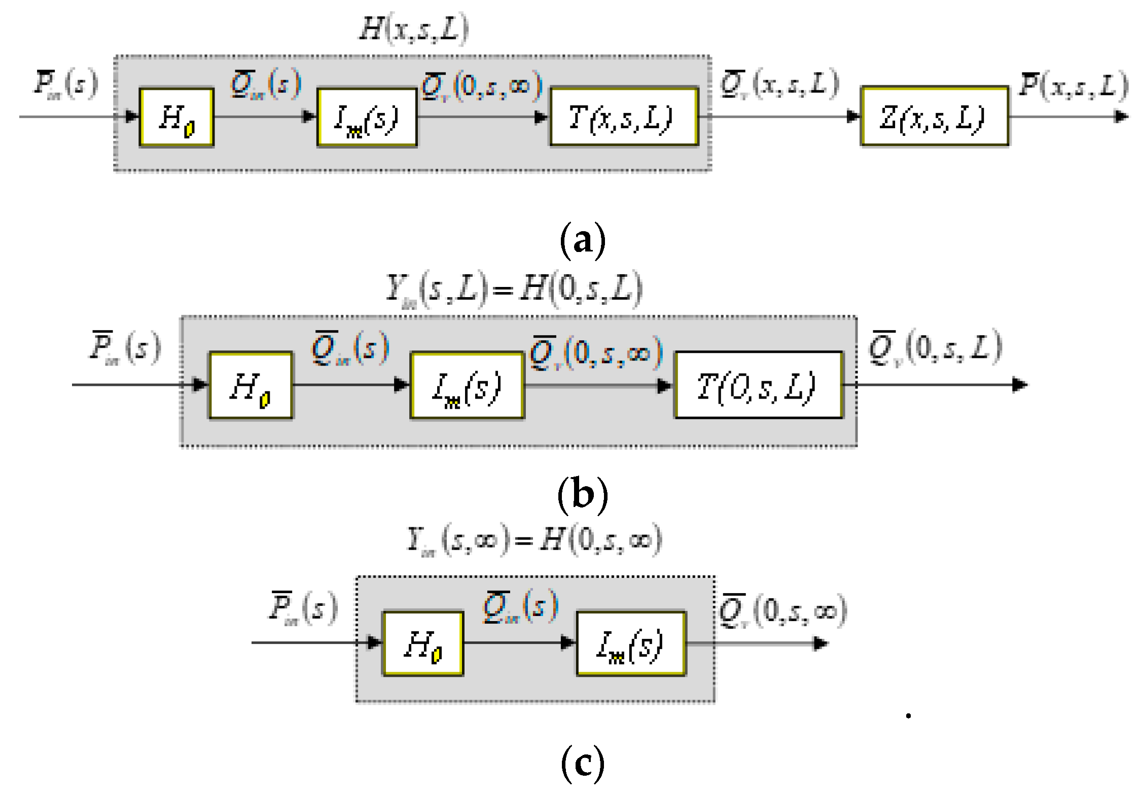
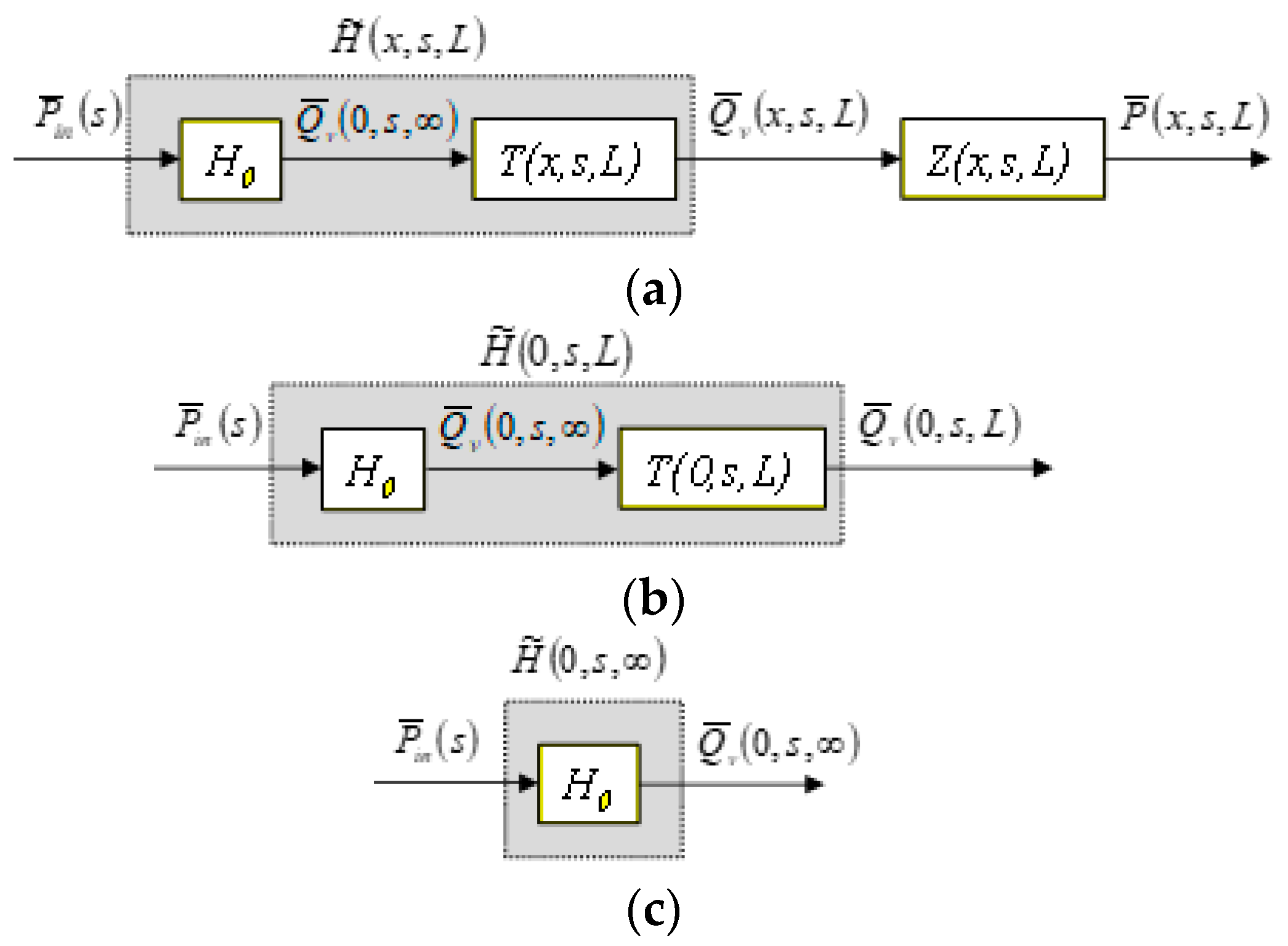
Figure 2 presents the block diagrams associated with this system approach where the different transfer functions are defined by:

$$\{\begin{array}{l}\begin{array}{l}{H}_0=\frac{{\overline{Q}}_{in}\left(s\right)}{{\overline{P}}_{in}\left(s\right)}=\hspace{0.17em}\frac{S}{Z_{ac}}\hspace{0.17em}=\hspace{0.17em}\hspace{0.17em}cste\\ I_m\left(s\right)=\frac{{\overline{Q}}_v\left(0,s,\infty \right)}{{\overline{Q}}_{in}\left(s\right)}=\hspace{0.17em}\sqrt{\frac{1\hspace{0.17em}+\hspace{0.17em}{\left(\frac{s}{{\omega }_{r,m}}\right)}^m}{{\left(\frac{s}{{\omega }_{r,m}}\right)}^m}}\end{array}\hfill \\ T\left(x,s,L\right)=\frac{{\overline{Q}}_v\left(x,s,L\right)}{{\overline{Q}}_v\left(0,s,\infty \right)}=\hspace{0.17em}\frac{1}{\tanh \left(\left(\frac{s}{{\omega }_{L,x}}\right)\hspace{0.17em}{I}_m\left(s\right)\right)}\hfill \end{array}.$$

(27)

Note that the quantity $H_0\hspace{0.17em}{\overline{P}}_{in}\left(s\right)$ is homogeneous at a flow, noted ${\overline{Q}}_{in}\left(s\right)$, corresponding to the conversion of the pressure source applied in x = 0 (Dirichlet condition) into an equivalent source of flow always applied in x = 0 (Neumann condition) [30].

3.2. Frequency Analysis of the System Approach

In a stationary harmonic regime, the relation (24) becomes:

$$H\left(x,j\omega ,L\right)=\frac{{\overline{Q}}_v\left(x,j\omega ,L\right)}{{\overline{P}}_{in}\left(j\omega \right)}=H_0\hspace{0.17em}{I}_m\left(j\omega \right)\hspace{0.17em}\hspace{0.17em}T\left(x,j\omega ,L\right)$$

(28)

with

$$I_m\left(j\omega \right)=\frac{{\overline{Q}}_v\left(0,j\omega ,\infty \right)}{{\overline{Q}}_{in}\left(j\omega \right)}=\hspace{0.17em}\sqrt{\frac{1\hspace{0.17em}+\hspace{0.17em}{\left(j\frac{\omega }{{\omega }_{r,m}}\right)}^m}{{\left(j\frac{\omega }{{\omega }_{r,m}}\right)}^m}}\hspace{0.17em}\hspace{0.17em}$$

(29)

and

$$T\left(x,j\omega ,L\right)=\frac{{\overline{Q}}_v\left(x,j\omega ,L\right)}{{\overline{Q}}_v\left(0,j\omega ,\infty \right)}=\hspace{0.17em}\frac{1}{\tanh \left(F\left(x,j\omega ,L\right)\right)}$$

(30)

where,

$$F\left(x,j\omega ,L\right)=\left(\frac{j\omega }{{\omega }_{L,x}}\right)\hspace{0.17em}\hspace{0.17em}{I}_m\left(j\omega \right).$$

(31)

The remaining part of this paragraph is devoted to a detailed analysis of the frequency responses I_m(jω), F(x,jω,L), and T(x,jω,L) of each subsystem. An analysis of the whole system response H(x,jω,L) will be also discussed.

3.2.1. Analysis of I_m(jω)

The analysis of I_m(jω) highlights two behaviors whose transition zone is fixed by the transitional frequency ω_r,m; these behaviors are:

• For ω << ω_r,m, a fractional integrative behavior of order m/2 = 0.25. Indeed,

$$\forall \hspace{0.17em}\omega \hspace{0.17em}<<\hspace{0.17em}{\omega }_{r,m}\hspace{0.17em},\hspace{1em}{I}_m\left(j\omega \right)=\hspace{0.17em}\sqrt{\frac{1\hspace{0.17em}+\hspace{0.17em}{\left(j\frac{\omega }{{\omega }_{r,m}}\right)}^m}{{\left(j\frac{\omega }{{\omega }_{r,m}}\right)}^m}\hspace{0.17em}}\underset{\omega \hspace{0.17em}<<\hspace{0.17em}{\omega }_{r,m}}{{\displaystyle \approx }}\hspace{0.17em}{\left(\frac{{\omega }_{r,m}}{j\omega }\right)}^{m/2}\hspace{1em}\Rightarrow \hspace{1em}\{\begin{array}{l}\left|I_m\left(j\omega \right)\right|=\hspace{0.17em}{\left(\frac{{\omega }_{r,m}}{\omega }\right)}^{m/2}\hfill \\ \arg I_m\left(j\omega \right)=\hspace{0.17em}-m\frac{\pi }{4}\hfill \end{array}.$$

(32)

• For ω >> ω_r,m, unitary proportional behavior. Indeed,

$$\forall \hspace{0.17em}\omega \hspace{0.17em}>>\hspace{0.17em}{\omega }_{r,m}\hspace{0.17em},\hspace{1em}{I}_m\left(j\omega \right)=\hspace{0.17em}\sqrt{\frac{1\hspace{0.17em}+\hspace{0.17em}{\left(j\frac{\omega }{{\omega }_{r,m}}\right)}^m}{{\left(j\frac{\omega }{{\omega }_{r,m}}\right)}^m}\hspace{0.17em}}\underset{\omega \hspace{0.17em}<<\hspace{0.17em}{\omega }_{r,m}}{{\displaystyle \approx }}\hspace{0.17em}1\hspace{1em}\Rightarrow \hspace{1em}\{\begin{array}{l}\left|I_m\left(j\omega \right)\right|=\hspace{0.17em}1\hfill \\ \arg I_m\left(j\omega \right)=\hspace{0.17em}0\hfill \end{array}.$$

(33)

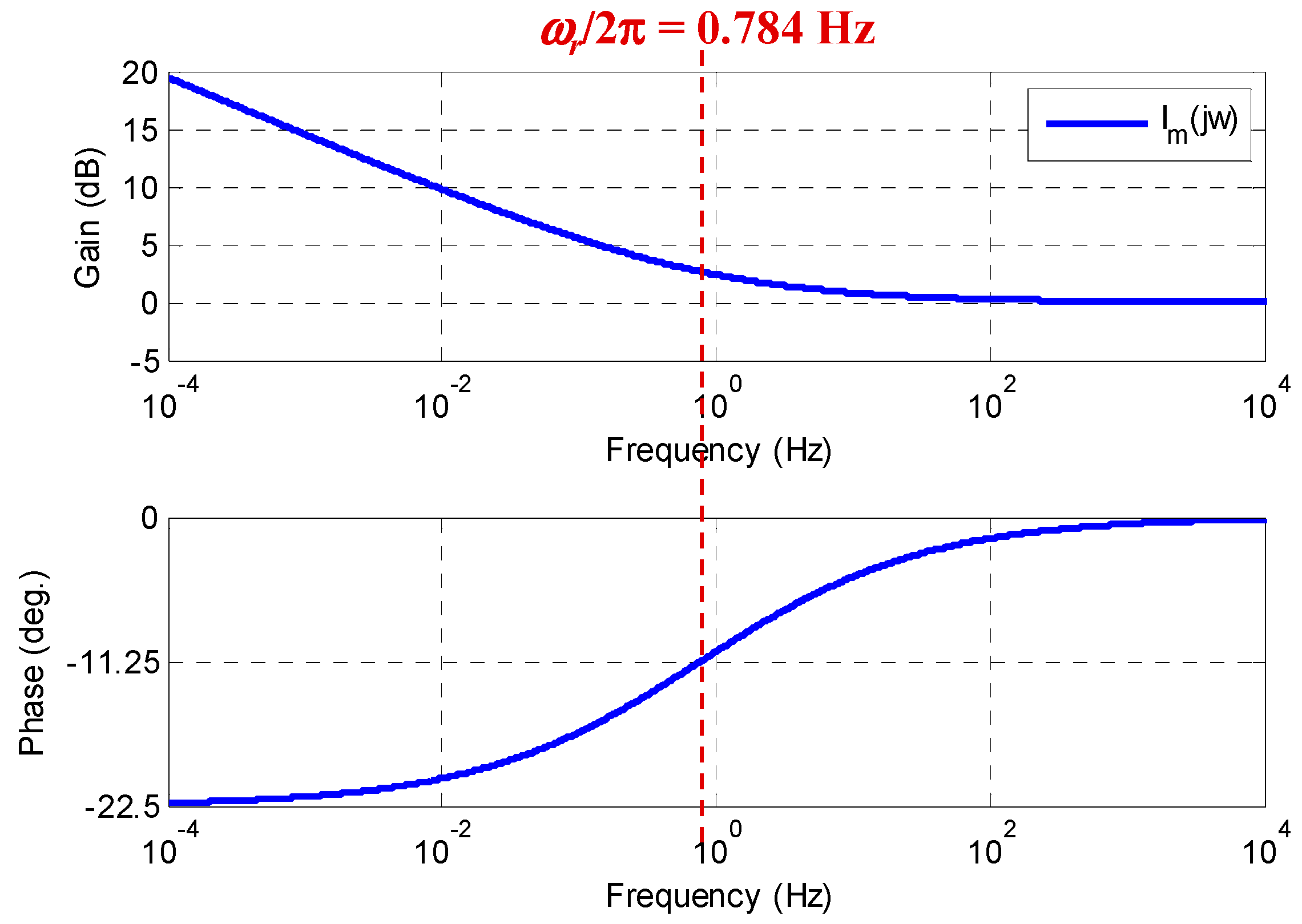
As an illustration, let us take the acoustic tube whose nominal dimensions are fixed by a radius r = 5 × 10⁻³ m and a length L = 0.3 m at a temperature of 25 °C, with ρ_a = 1.184 kg/m³ and c_a = 346.3 m/s. In this case, and as a reminder, the numerical value of the transitional frequency ω_r,m (relation (33)) and 4.92 rad/s (0.784 Hz).

The values of r = 5 mm and L = 0.3 m correspond to the dimensions of the experimental device developed in a first part of the overall project and used to validate a numerical simulator of the artificial mouth + nonlinear exciter + resonator assembly, in addition to a simulator developed using MatLab/Simulink.

Figure 3 presents the Bode diagrams of the frequency response I_m(jω) over the range [10⁻⁴; 10⁴] Hz. The two behaviors appear clearly with:

• For ω << ω_r,m, a gain diagram with a straight line with slope p = −m/2 × 20 dB/dec = −5 dB/dec and a phase diagram with a horizontal line at −m/2 × 90° = −22.5°;
• For ω >> ω_r,m, a gain diagram with a horizontal line at 0 dB and a phase diagram with a horizontal line at 0°.

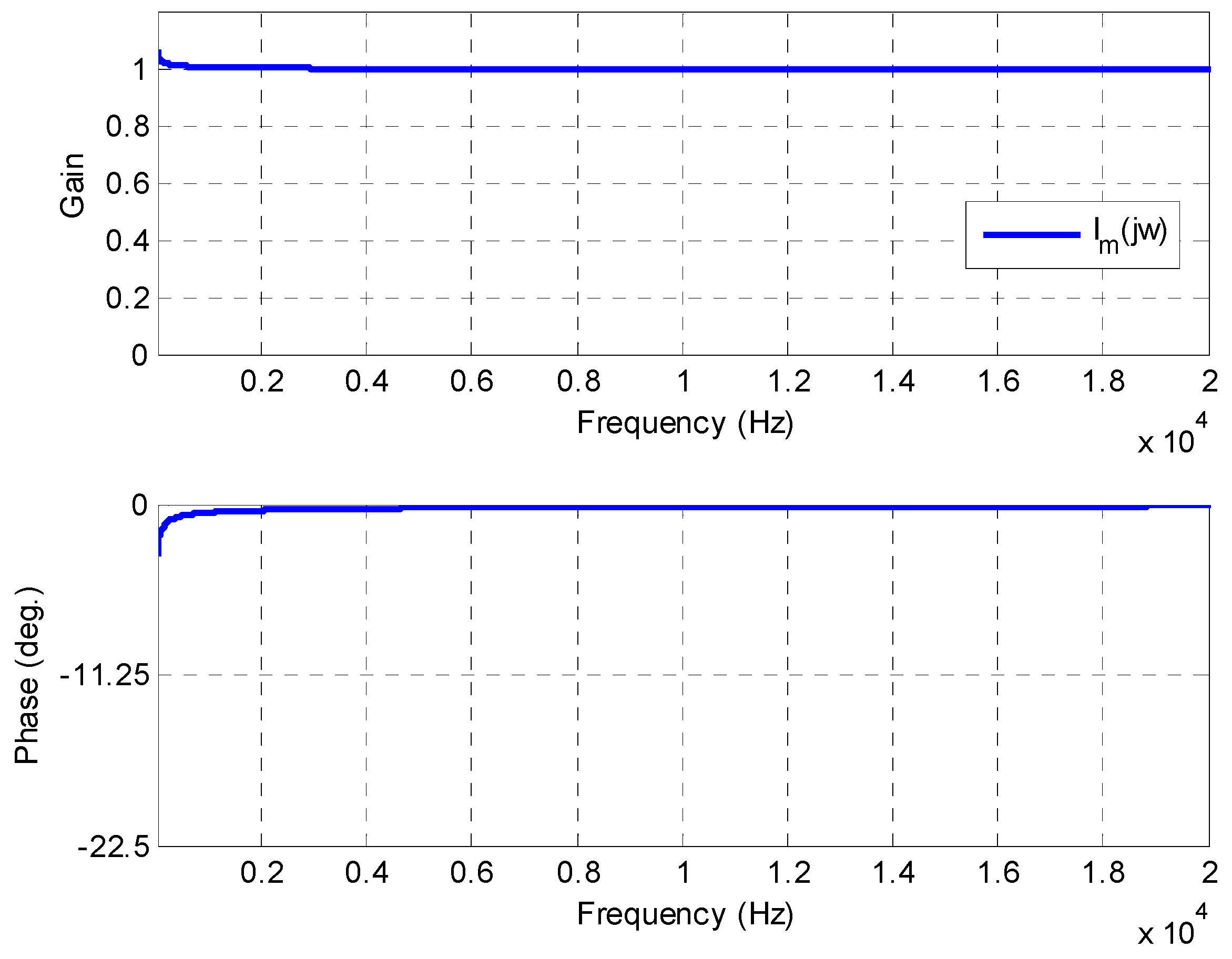
Figure 4 presents the same frequency response of I_m(jω) but only over the audible frequency range [20–20,000] Hz. The gain diagram is in linear–linear scale and a phase diagram with the frequency axis is also in linear scale. This result makes it possible to confirm, for this recorder example, that the unit proportional behavior is dominant, that is:

$$\forall \hspace{0.17em}\hspace{0.17em}\hspace{0.17em}\omega \hspace{0.17em}\hspace{0.17em}\ge \hspace{0.17em}\hspace{0.17em}2\pi \hspace{0.17em}20\hspace{0.17em}\hspace{0.17em}\mathrm{rad}/\mathrm{s}\hspace{0.17em},\hspace{1em}{I}_m\left(j\omega \right)=\frac{{\overline{Q}}_v\left(0,j\omega ,\infty \right)}{{\overline{Q}}_{in}\left(j\omega \right)}\approx \hspace{0.17em}1\hspace{0.17em}\hspace{0.17em}.$$

(34)

Thus, for the area of study considered in this work, the area defined by the range [20–20,000] Hz of the audible frequencies, the transfer I_m(s) can be reduced to the unit, which amounts to writing ${\overline{Q}}_v\left(0,s,\infty \right)={\overline{Q}}_{in}\left(s\right)$, allowing a reduction in the block diagrams of Figure 2. The direct consequence is that in the case of a semi-infinite medium at x = 0, the fractional integration behavior has no influence on the range of audible frequencies.

3.2.2. Analysis of F(0,jω,L)

Knowing that in the case of a recorder ω_r,m << ω_L,x, the analysis of F(0,jω,L) again highlights two behaviors whose transition zone is fixed by the transitional frequency ω_r,m, that is:

• For ω << ω_r,m, a fractional derivative behavior of order (1 − m/2) = 0.75. Indeed,

$$\forall \hspace{0.17em}\omega \hspace{0.17em}<<\hspace{0.17em}{\omega }_{r,m}\hspace{0.17em},\hspace{1em}F\left(x,j\omega ,L\right)=\hspace{0.17em}\left(\frac{j\omega }{{\omega }_{L,x}}\right)\sqrt{\frac{1\hspace{0.17em}+\hspace{0.17em}{\left(j\frac{\omega }{{\omega }_{r,m}}\right)}^m}{{\left(j\frac{\omega }{{\omega }_{r,m}}\right)}^m}\hspace{0.17em}}\underset{\omega \hspace{0.17em}<<\hspace{0.17em}{\omega }_{r,m}}{{\displaystyle \approx }}\hspace{0.17em}\left(\frac{{\omega }_{r,m}^{m/2}}{{\omega }_{L,x}}\right)\hspace{0.17em}{\left(j\omega \right)}^{\left(1-m/2\right)}$$

(35)

• Hence, the module and the argument

$$\{\begin{array}{l}\left|F\left(x,j\omega ,L\right)\right|=\hspace{0.17em}\left(\frac{{\omega }_{r,m}^{m/2}}{{\omega }_{L,x}}\right)\hspace{0.17em}{\omega }^{\left(1-m/2\right)}\hfill \\ \arg F\left(x,j\omega ,L\right)=\hspace{0.17em}\left(1-\frac{m}{2}\right)\frac{\pi }{2}\hfill \end{array}.$$

(36)

• For ω_r << ω, a derivative behavior of order 1. Indeed,

$$\forall \hspace{0.17em}{\omega }_{r,m}\hspace{0.17em}<<\hspace{0.17em}\omega \hspace{0.17em},\hspace{1em}F\left(x,j\omega ,L\right)=\hspace{0.17em}\left(\frac{j\omega }{{\omega }_{L,x}}\right)\sqrt{\frac{1\hspace{0.17em}+\hspace{0.17em}{\left(j\frac{\omega }{{\omega }_{r,m}}\right)}^m}{{\left(j\frac{\omega }{{\omega }_{r,m}}\right)}^m}\hspace{0.17em}}\underset{{\omega }_{r,m}\hspace{0.17em}<<\hspace{0.17em}\omega }{{\displaystyle \approx }}\hspace{0.17em}\left(\frac{j\omega }{{\omega }_{L,x}}\right)\hspace{0.17em}\hspace{0.17em}\Rightarrow \hspace{0.17em}\hspace{0.17em}\{\begin{array}{l}\left|F\left(x,j\omega ,L\right)\right|=\frac{\omega }{{\omega }_{L,x}}\hfill \\ \arg F\left(x,j\omega ,L\right)=\hspace{0.17em}\frac{\pi }{2}\hfill \end{array}.$$

(37)

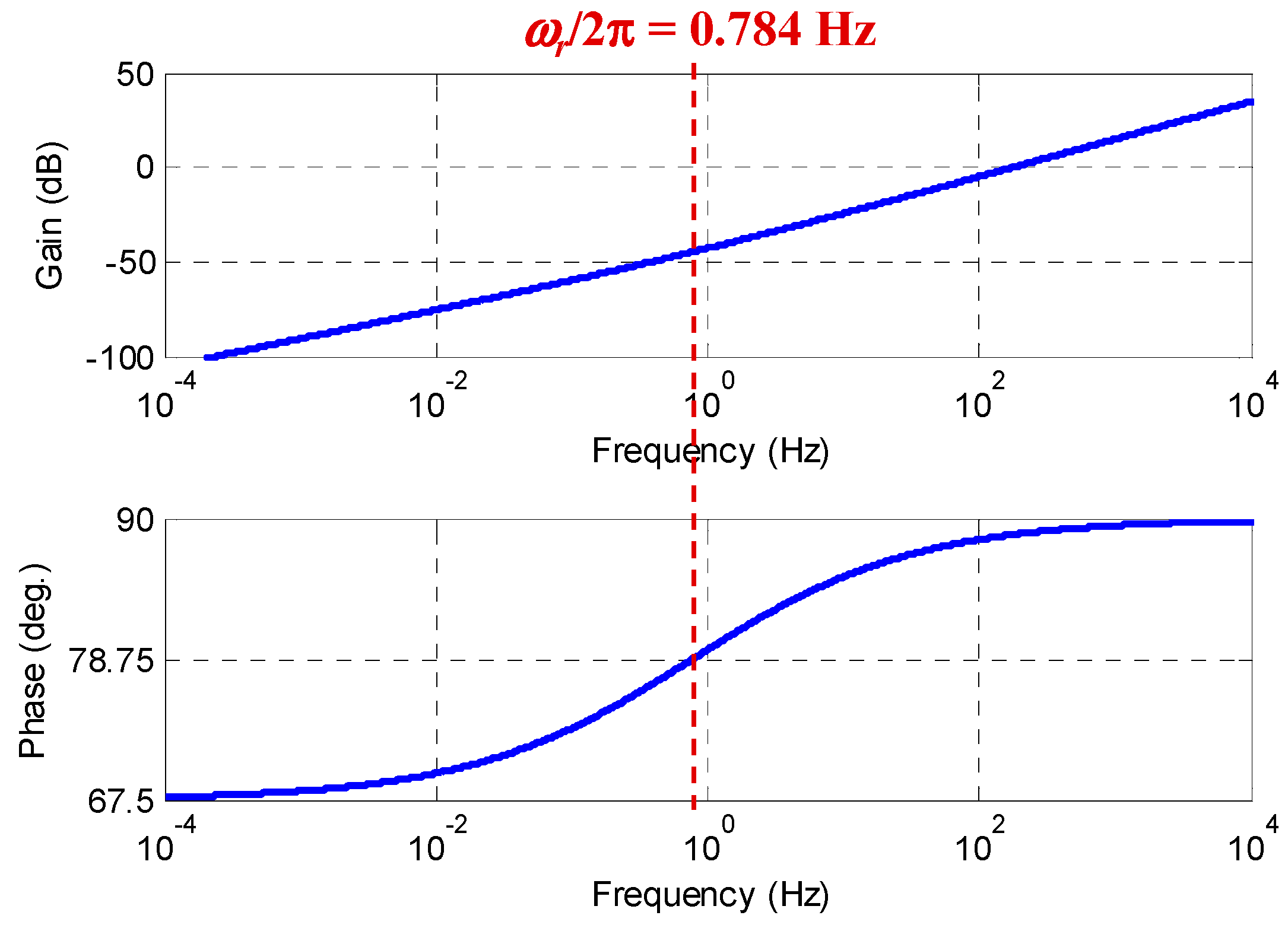
Figure 5 presents in x = 0 the Bode diagrams of the frequency response F(0,jω,L) on the range [10⁻⁴; 10⁴] Hz. The two behaviors appear clearly:

• For ω << ω_r,m, a gain diagram with a straight line with p₁ = (1 − m/2) × 20 dB/dec = 15 dB/dec and a phase diagram with a horizontal line at (1 − m/2) × 90° = 67.5°;
• For ω >> ω_r,m, a gain diagram with a straight line with slope p₂ = 20 dB/dec and a phase diagram with a horizontal straight line at 90°.

3.2.3. Analysis of T(0,jω,L)

The analysis of T(x,jω,L) highlights three behaviors whose transition zones are fixed by the transitional frequencies ω_r,m and ω_L,x:

• For w << ω_L,x, an integrative behavior with two different orders according to the frequency range. Indeed,

$$\forall \hspace{0.17em}\omega \hspace{0.17em}<<\hspace{0.17em}{\omega }_{L,x}\hspace{0.17em},\hspace{1em}T\left(x,j\omega ,L\right)=\hspace{0.17em}\frac{1}{\tanh \left(F\left(x,j\omega ,L\right)\right)}\underset{\omega \hspace{0.17em}<<\hspace{0.17em}{\omega }_{L,x}}{{\displaystyle \approx }}\hspace{0.17em}\frac{1}{F\left(x,j\omega ,L\right)}$$

(38)

with, for ω << ω_r,m, an orderly fractional integrative behavior—(1 − m/2) = −0.75, that is

$$\forall \hspace{0.17em}\omega \hspace{0.17em}<<\hspace{0.17em}{\omega }_{r,m}\hspace{0.17em},\hspace{1em}\frac{1}{F\left(x,j\omega ,L\right)}\underset{\omega \hspace{0.17em}<<\hspace{0.17em}{\omega }_{r,m}}{{\displaystyle \approx }}\hspace{0.17em}\left(\frac{{\omega }_{L,x}}{{\omega }_r^{m/2}}\right)\hspace{0.17em}\frac{1}{{\left(j\omega \right)}^{\left(1-m/2\right)}}\hspace{0.17em}\hspace{0.17em}\Rightarrow \hspace{0.17em}\hspace{0.17em}\{\begin{array}{l}\left|T\left(x,j\omega ,L\right)\right|=\hspace{0.17em}\left(\frac{{\omega }_{L,x}}{{\omega }_r^{m/2}}\right)\hspace{0.17em}\frac{1}{{\omega }^{\left(1-m/2\right)}}\hfill \\ \arg T\left(x,j\omega ,L\right)=\hspace{0.17em}\left(1-\frac{m}{2}\right)\frac{\pi }{2}\hfill \end{array}$$

(39)

and, for ω_r,m << ω, a derivative behavior of order 1, that is

$$\forall \hspace{0.17em}{\omega }_{r,m}\hspace{0.17em}<<\hspace{0.17em}\omega \hspace{0.17em},\hspace{1em}\frac{1}{F\left(x,j\omega ,L\right)}\underset{{\omega }_{r,m}\hspace{0.17em}<<\hspace{0.17em}\omega }{{\displaystyle \approx }}\hspace{0.17em}\left(\frac{{\omega }_{L,x}}{j\omega }\right)\hspace{0.17em}\hspace{0.17em}\Rightarrow \hspace{0.17em}\hspace{0.17em}\{\begin{array}{l}\left|T\left(x,j\omega ,L\right)\right|=\frac{{\omega }_{L,x}}{\omega }\hfill \\ \arg T\left(x,j\omega ,L\right)=\hspace{0.17em}-\frac{\pi }{2}\hfill \end{array}.$$

(40)

• For ω_L,x << ω, a behavior composed of an alternation of anti-resonances and resonances, and this without there being a simplification of the expression of T(x,jω,L) is:

$$\forall \hspace{0.17em}{\omega }_{L,x}\hspace{0.17em}<<\hspace{0.17em}\omega \hspace{0.17em},\hspace{1em}T\left(x,j\omega ,L\right)=\hspace{0.17em}\frac{1}{\tanh \left(\left(\frac{j\omega }{{\omega }_{L,x}}\right)\sqrt{\frac{1\hspace{0.17em}+\hspace{0.17em}{\left(j\frac{\omega }{{\omega }_{r,m}}\right)}^m}{{\left(j\frac{\omega }{{\omega }_{r,m}}\right)}^m}\hspace{0.17em}}\right)}.$$

(41)

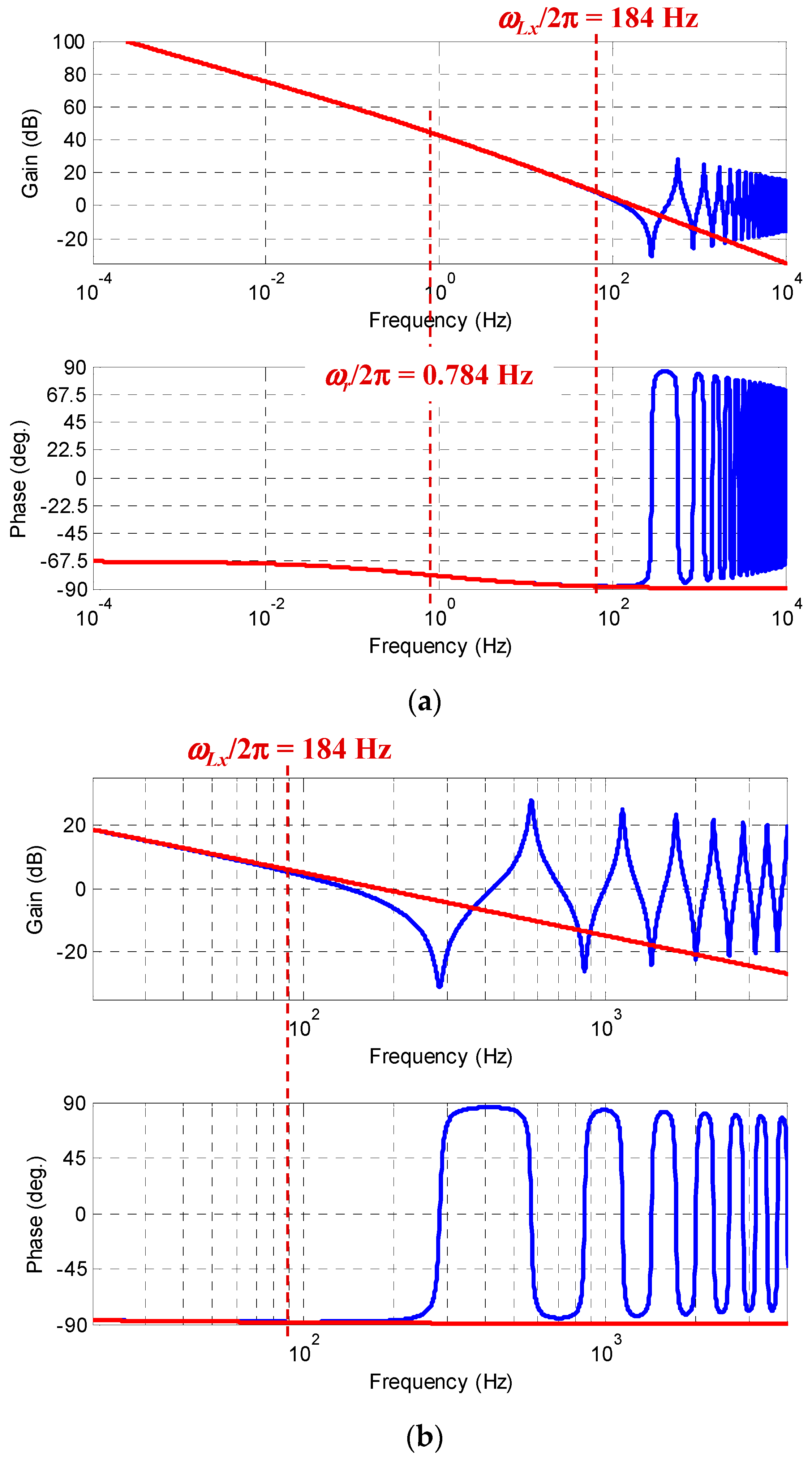
Figure 6 shows the Bode diagrams of 1/F(0,jω,L) (in red) and of T(0,jω,L) (in blue) over the range [10⁻⁴; 10⁴] Hz (Figure 6a) and on the range [20–4000] Hz of the audible and achievable frequencies with a recorder (Figure 6b).

Below the first cutoff frequency [10⁻⁴; ω_L,x/2π = 184] Hz, the responses of 1/F(0,jω,L) (in red) and T(0,jω,L) (in blue) overlap where:

• A fractional integration behavior of order −0.75 over the range [10⁻⁴; ω_r/2π = 0.784] Hz is observed;
• An integrative behavior of order 1 over the range [ω_r,m/2π = 0.784; ω_L,x/2π = 184] Hz is observed.

Beyond 184 Hz, the frequency response T(0,jω,L) (in blue) clearly presents an alternation of anti-resonances and resonances introduced by the hyperbolic tangent function.

3.2.4. Analysis of H(x,jω,L)

The analysis of H(x,jω,L) highlights three behaviors whose transition zones are fixed by the transitional frequencies ω_r and ω_L,x:

• For ω << ω_r << ω_L,x, an orderly fractional integrative behavior—(1 − m/2) = −0.75, that is

$$\forall \hspace{0.17em}\omega \hspace{0.17em}<<\hspace{0.17em}{\omega }_{r,m}\hspace{0.17em},\hspace{1em}H\left(x,j\omega ,L\right)\underset{\omega \hspace{0.17em}<<\hspace{0.17em}{\omega }_{r,m}}{{\displaystyle \approx }}\hspace{0.17em}\left(\frac{{\omega }_{L,x}}{{\omega }_{r,m}^{m/2}}\right)\hspace{0.17em}\frac{H_0}{{\left(j\omega \right)}^{\left(1-m/2\right)}}\hspace{0.17em}\hspace{0.17em}\Rightarrow \hspace{0.17em}\hspace{0.17em}\{\begin{array}{l}\left|H\left(x,j\omega ,L\right)\right|=\hspace{0.17em}\left(\frac{{\omega }_{L,x}}{{\omega }_{r,m}^{m/2}}\right)\hspace{0.17em}\frac{H_0}{{\omega }^{\left(1-m/2\right)}}\hfill \\ \arg H\left(x,j\omega ,L\right)=\hspace{0.17em}\left(1-\frac{m}{2}\right)\frac{\pi }{2}\hfill \end{array}.$$

(42)

• For ω_r,m << ω << ω_L,x, a derivative behavior of order 1, that is

$$\forall \hspace{0.17em}{\omega }_{r,m}\hspace{0.17em}<<\hspace{0.17em}\omega \hspace{0.17em}<<{\omega }_{L,x},\hspace{1em}H\left(x,j\omega ,L\right)\underset{{\omega }_{r,m}\hspace{0.17em}<<\hspace{0.17em}\omega <<\hspace{0.17em}{\omega }_{L,x}}{{\displaystyle \approx }}\hspace{0.17em}{H}_0\hspace{0.17em}\left(\frac{{\omega }_{L,x}}{j\omega }\right)\hspace{0.17em}\hspace{0.17em}\Rightarrow \hspace{0.17em}\hspace{0.17em}\{\begin{array}{l}\left|H\left(x,j\omega ,L\right)\right|=H_0\hspace{0.17em}\frac{{\omega }_{L,x}}{\omega }\hfill \\ \arg H\left(x,j\omega ,L\right)=\hspace{0.17em}-\frac{\pi }{2}\hfill \end{array}$$

(43)

• For ω_L,x << ω, a behavior composed of an alternation of anti-resonances and resonances, that is,

$$\forall \hspace{0.17em}{\omega }_{L,x}\hspace{0.17em}<<\hspace{0.17em}\omega \hspace{0.17em},\hspace{1em}H\left(x,j\omega ,L\right)\underset{{\omega }_{L,x}\hspace{0.17em}<<\hspace{0.17em}\omega }{{\displaystyle \approx }}\hspace{0.17em}\frac{H_0}{\tanh \left(\left(\frac{j\omega }{{\omega }_{L,x}}\right)\sqrt{\frac{1\hspace{0.17em}+\hspace{0.17em}{\left(j\frac{\omega }{{\omega }_{r,m}}\right)}^m}{{\left(j\frac{\omega }{{\omega }_{r,m}}\right)}^m}\hspace{0.17em}}\right)}.$$

(44)

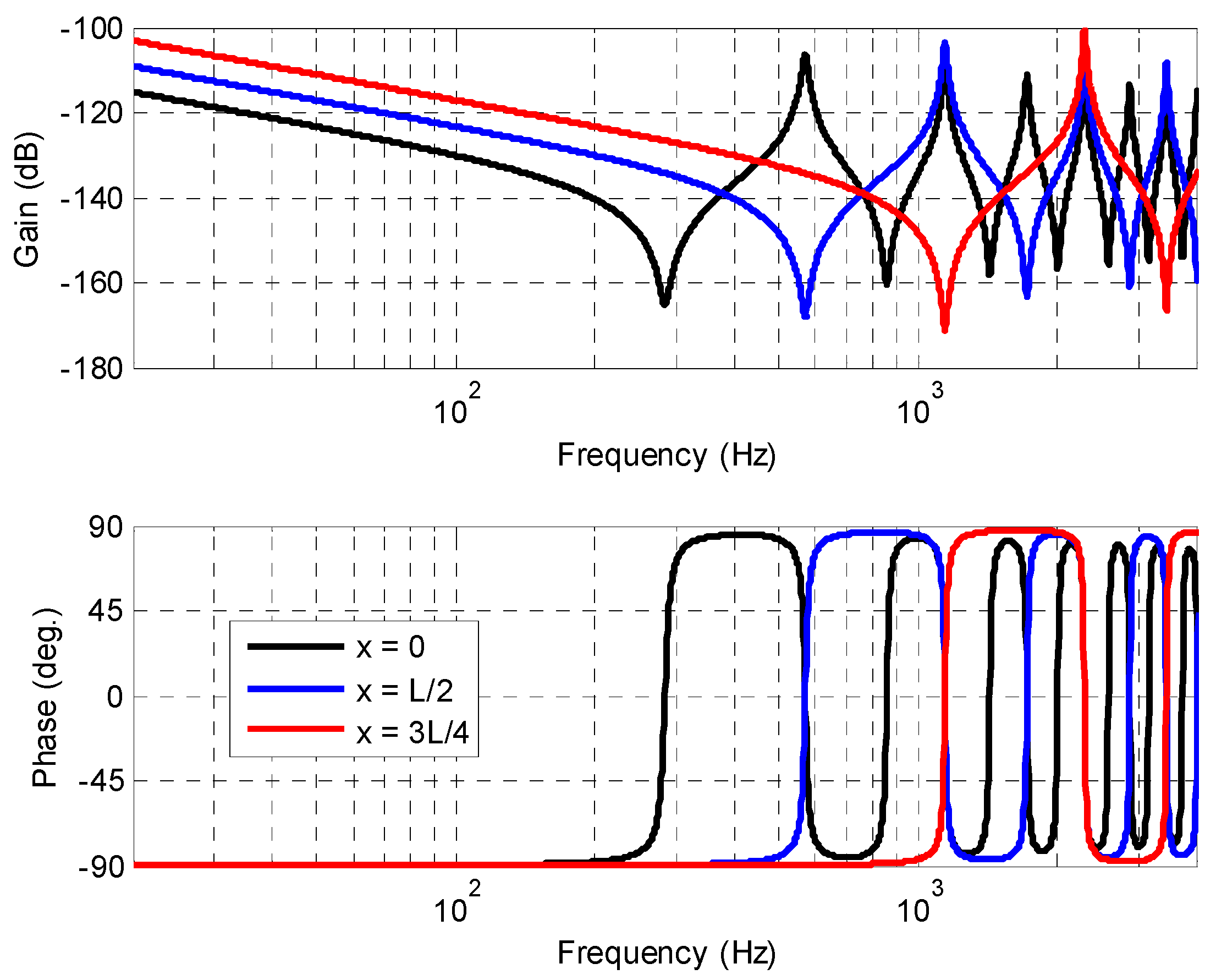
Figure 7 presents, at x = 0 (ω_L,x/2π = 184 Hz), at x = L/2 (ω_L,x/2π = 368 Hz), and at x = 3L/4 (ω_L,x/2π = 735 Hz), the Bode diagrams of H(0,jω,L) (in black), of H(L/2,jω,L) (in blue), and of H(3L/4,jω,L) (in red) over the audible frequency range [20–4000] Hz.

Over the range [20–ω_L,x/2π] Hz, the three responses of H(x,jω,L) present an integration behavior of order 1. The fractional integration behavior of order −0.75 does not appear over this range, as it is present within a much lower frequency (0.784 Hz). Beyond ω_L,x, the three responses present a succession of alternation of anti-resonances and resonances introduced by the hyperbolic tangent (tanh) function.

Note that the farther the position x moves away from the origin, the higher the transitional frequency ω_L,x pushes the anti-resonance and resonance frequencies toward the high frequencies.

In addition, the position x having no influence on the transitional frequency ω_r,m, the fractional integrative behavior of order −0.75 still does not appear in this frequency range.

3.3. Study of the Influence of the Fractional Order m

In the Webster–Lokshin model, the fractional order m has the value 0.5. The objective of this paragraph is to analyze the influence of the order m on the behavior of the resonator by considering that m belongs to the interval [0; 1] with a nominal value m₀ = 0.5, which is a consideration that facilitates the introduction of the concept of parametric uncertainty (additive or multiplicative) at the fractional order level. Thus, by generalizing the expression of the parameter ε = K₀/r associated with visco-thermal losses in the Webster–Lokshin model at ε = 2 m K₀/r which for m = 0.5 gives the same expression), the analytical link is naturally established between visco-thermal losses and fractional order.

Thus, the fractional order occurs only in the presence of visco-thermal losses. In the theoretical case of a purely conservative system, the parameter ε is zero, which is equivalent to m = 0, taking into account the relation (44). In this case, the expression of the acoustic transfer H (x, s, L), denoted then H₀ (x, s, L), of a finite medium is reduced to:

$$H_0\left(x,s,L\right)=\hspace{0.17em}\frac{H_0}{\tanh \left(\frac{s}{{\omega }_{L,x}}\right)}.$$

(45)

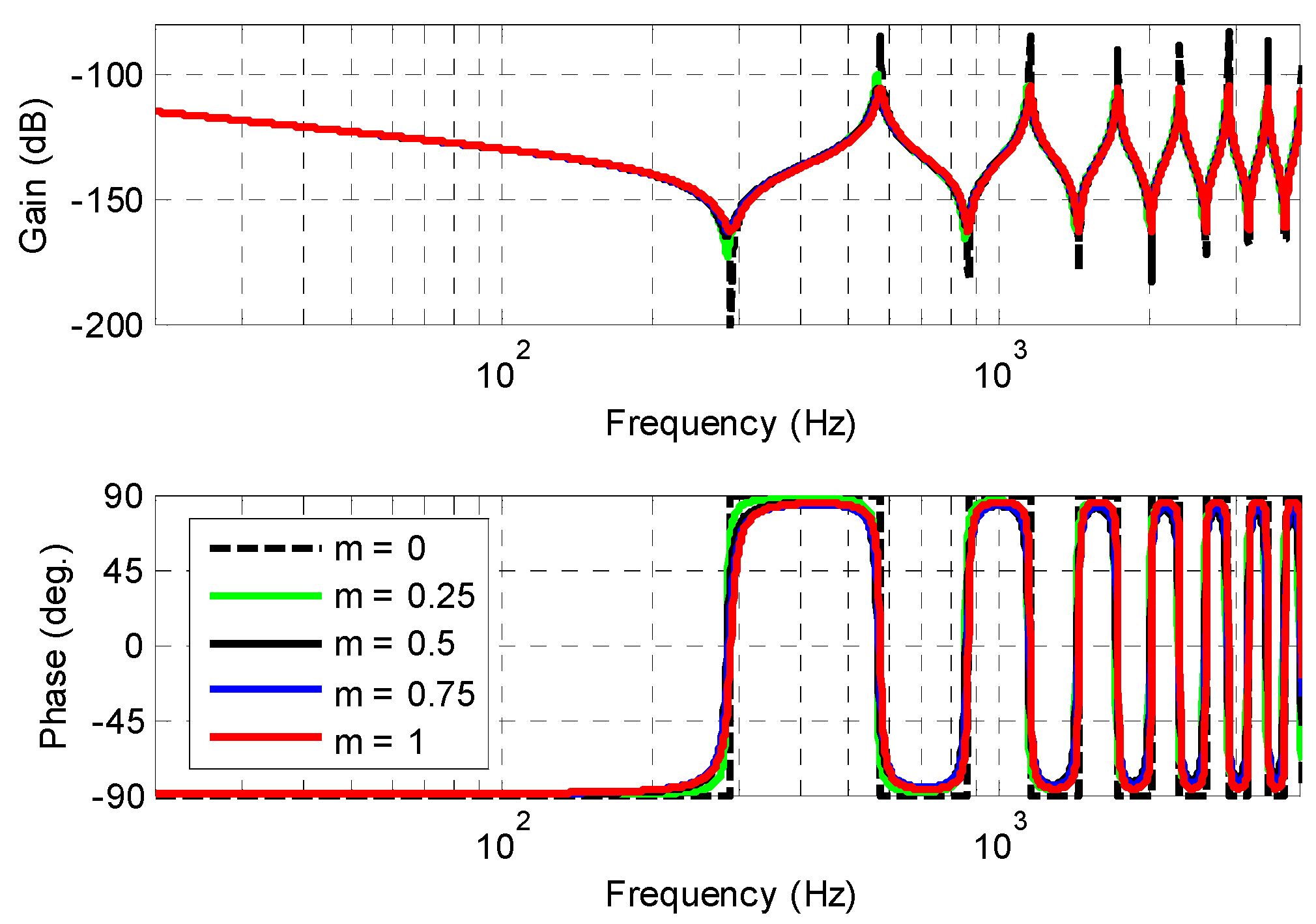
Figure 8 shows the Bode diagrams at x = 0 of H(0,jω,L) for different values of the fractional order over the range [20–4000] Hz of the audible and achievable frequencies with a recorder (Figure 7).

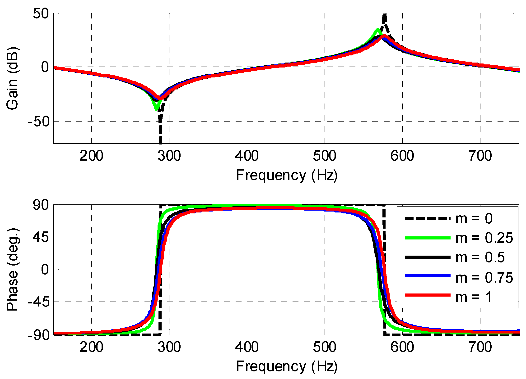
In order to magnify the different curves in Figure 8 for better observation, Figure 9 presents the reduced frequency responses H(0,jω,L)/H₀ with the frequency axis on a linear scale over the range [20–1000] Hz.

The observation of these frequency responses shows that the influence of the order m is essentially located:

• For gain diagrams, at the peaks of resonances and anti-resonances; quantifiable effects using quality factors Q_zi for anti-resonances and Q_pi for resonances clearly illustrate the phenomenon of dissipation associated with visco-thermal losses.
• For phase diagrams, at the crossing points at 0° with a local slope, which is all the more important as the order is small, and the slope becomes infinite for m = 0 (purely conservative case).

4. From the Simplified Fractional Model to its Rational Forms

For the area of study defined by the range [20–20,000] Hz of the audible frequencies, the analysis presented in the previous paragraph shows that the frequency response I_m(jω) is:

$$I_m\left(j\omega \right)=\hspace{0.17em}\sqrt{\frac{1\hspace{0.17em}+\hspace{0.17em}{\left(j\frac{\omega }{{\omega }_{r,m}}\right)}^m}{{\left(j\frac{\omega }{{\omega }_{r,m}}\right)}^m}\hspace{0.17em}}$$

(46)

which can be reduced to the unit. This is the reason why for this field of study, the frequency response H(x,jω,L) defined, as a reminder, by

$$H\left(x,j\omega ,L\right)=\frac{{\overline{Q}}_v\left(x,j\omega ,L\right)}{{\overline{P}}_{in}\left(j\omega \right)}=H_0\hspace{0.17em}{I}_m\left(j\omega \right)\hspace{0.17em}\hspace{0.17em}T\left(x,j\omega ,L\right)$$

(47)

is simplified and noted as $\tilde{H}\left(x,j\omega ,L\right)$, that is:

$$\tilde{H}\left(x,j\omega ,L\right)=H_0\hspace{0.17em}T\left(x,j\omega ,L\right)$$

(48)

with, always as a reminder,

$$T\left(x,j\omega ,L\right)=\hspace{0.17em}\frac{\tilde{H}\left(x,j\omega ,L\right)}{H_0}\hspace{0.17em}=\hspace{0.17em}\frac{1}{\tanh \left(\left(\frac{j\omega }{{\omega }_{L,x}}\right)\hspace{0.17em}{I}_m\left(j\omega \right)\right)}\hspace{0.17em}=\hspace{0.17em}\mathrm{cotanh}\left(\left(\frac{j\omega }{{\omega }_{L,x}}\right)\hspace{0.17em}{I}_m\left(j\omega \right)\right).$$

(49)

Figure 10 shows the block diagrams associated with this simplification in the field of study.

In general, the temporal simulation of fractional models often requires the use of rational models [30]. Thus, the fractional form of defined by the relation (49) can be put in a rational form of N cells in cascade, noted ${\tilde{H}}_{N,c}\left(x,s,L\right)$, that is:

$${\tilde{H}}_{N,c}\left(x,s,L\right)\hspace{0.17em}=\hspace{0.17em}\frac{A_0}{s}\hspace{0.17em}{\displaystyle \prod _{i=1}^N\left(\frac{1+2\hspace{0.17em}{\zeta }_{zi}\hspace{0.17em}\frac{s}{{\omega }_{zi}}+{\left(\frac{s}{{\omega }_{zi}}\right)}^2}{1+2\hspace{0.17em}{\zeta }_{pi}\hspace{0.17em}\frac{s}{{\omega }_{pi}}+{\left(\frac{s}{{\omega }_{pi}}\right)}^2}\right)}$$

(50)

or in a rational form of N cells in parallel, noted ${\tilde{H}}_{N,p}\left(x,s,L\right)$, either:

$${\tilde{H}}_{N,p}\left(x,s,L\right)\hspace{0.17em}=\hspace{0.17em}\frac{A_0}{s}\hspace{0.17em}+\hspace{0.17em}{\displaystyle \sum _{i=1}^N\left(\frac{A_i\hspace{0.17em}s+B_i}{1+2\hspace{0.17em}{\zeta }_{pi}\hspace{0.17em}\frac{s}{{\omega }_{pi}}+{\left(\frac{s}{{\omega }_{pi}}\right)}^2}\right)}$$

(51)

with A₀ = H₀ ω_L,x and where the ω_zi and ζ_zi represent the frequencies and the damping factors associated with the anti-resonances, ω_pi and ζ_pi represent the frequencies and the damping factors associated with the resonances, the passage from the cascade form (50) to the parallel form (51) by decomposing into simple elements. Note that the parallel rational form facilitates the return to the time domain by inverse Laplace transform, and that it is often associated with a decomposition in a modal space [31].

From a theoretical point of view, the ω_zi corresponds to the roots of the numerator of T(x,jω,L), that is:

$$\cosh \left(\left(\frac{j\omega }{{\omega }_{L,x}}\right)\hspace{0.17em}\sqrt{\frac{1\hspace{0.17em}+\hspace{0.17em}{\left(j\frac{\omega }{{\omega }_{r,m}}\right)}^m}{{\left(j\frac{\omega }{{\omega }_{r,m}}\right)}^m}\hspace{0.17em}}\right)\hspace{0.17em}=\hspace{0.17em}0$$

(52)

and the ω_pi corresponds to the roots of the denominator of T(x,jω,L), that is:

$$\sinh \left(\left(\frac{j\omega }{{\omega }_{L,x}}\right)\hspace{0.17em}\sqrt{\frac{1\hspace{0.17em}+\hspace{0.17em}{\left(j\frac{\omega }{{\omega }_{r,m}}\right)}^m}{{\left(j\frac{\omega }{{\omega }_{r,m}}\right)}^m}\hspace{0.17em}}\right)\hspace{0.17em}=\hspace{0.17em}0.$$

(53)

From a practical point of view, finding these roots by analytical resolution is complex, if not impossible. On the other hand, the search by numerical resolution does not pose any particular problem. For example, it is possible to use the fact that the alternation of ω_zi and ω_pi appears clearly on the phase from when passing at 0° from −90° to +90° for ω_zi and from +90° to −90° for ω_pi (see example illustration below).

In the context of the work of this thesis, the rational forms of N cells in cascade and in parallel are considered as behavior models whose numerical values of the parameters are obtained using an optimal approach aiming to minimize the difference between the target frequency response defined by the fractional form $\tilde{H}\left(x,s,L\right)$ and the frequency response of the rational cascade form ${\tilde{H}}_{N,c}\left(x,s,L\right)$. This digital procedure is available in the Frequency Domain System Identification (FDSI) module of the CRONE Toolbox [32].

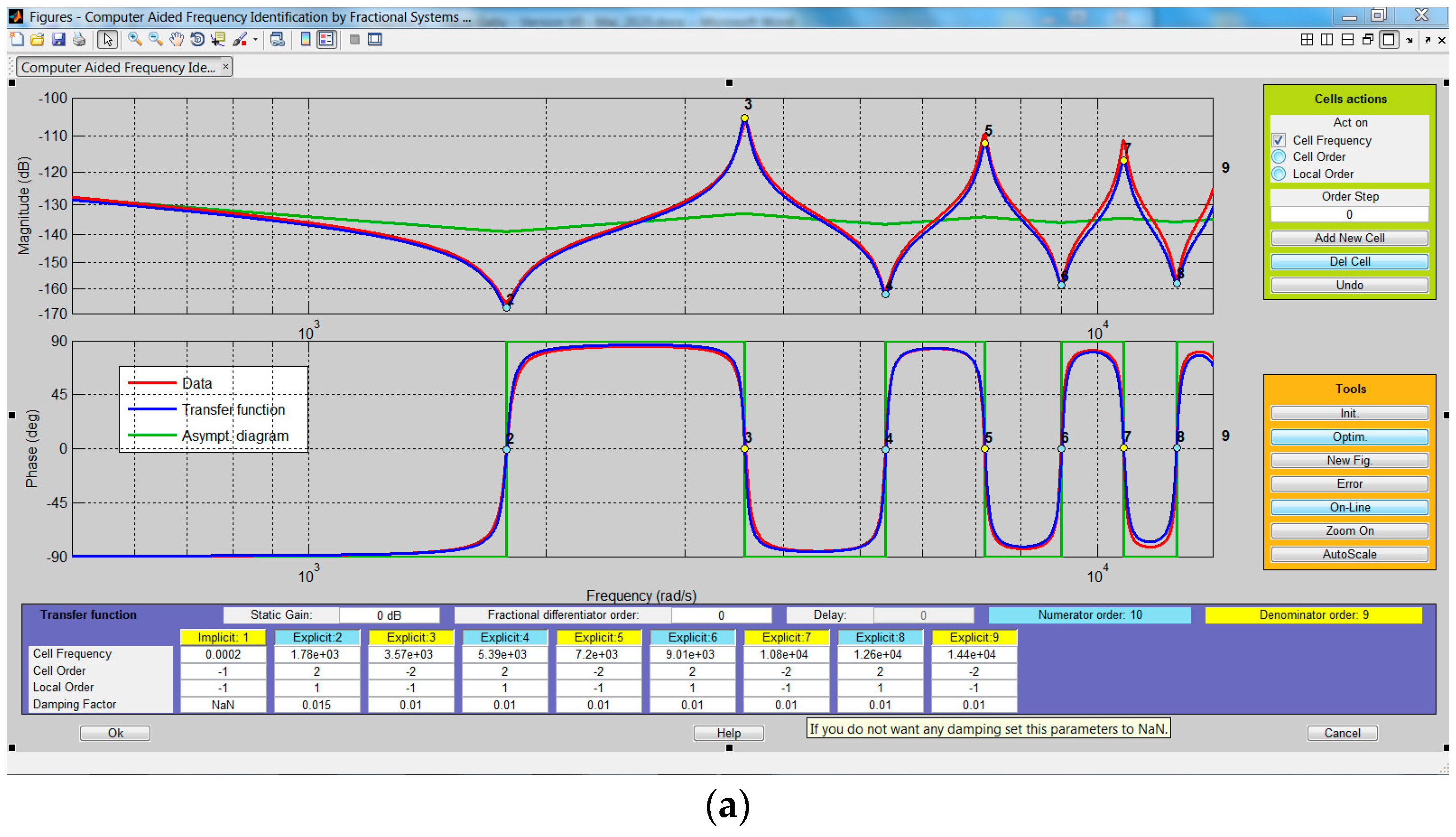
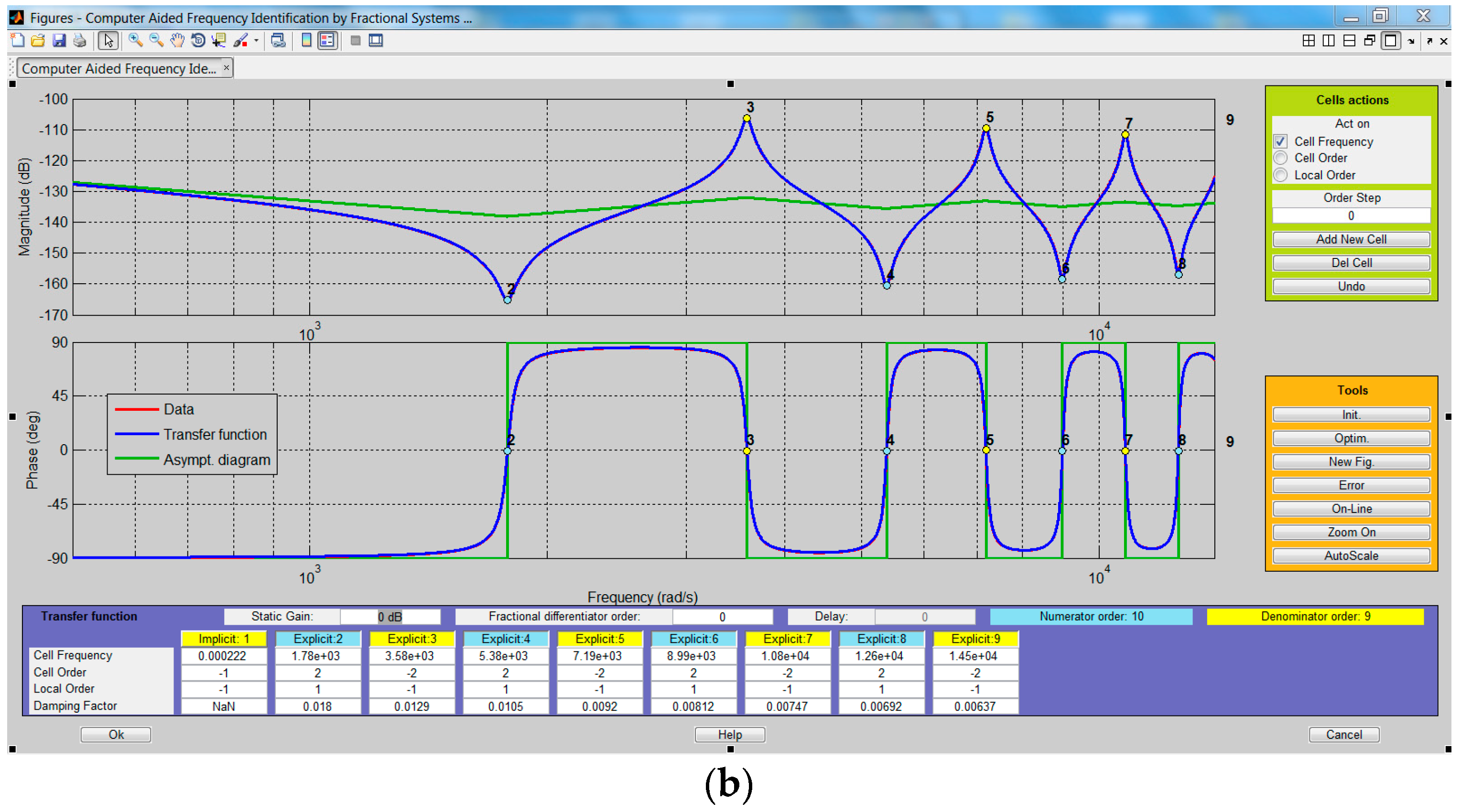
As an illustration, let us take the acoustic tube used as an example throughout this article, either: r = 5 × 10⁻³ m, L = 0.3 m, ρ_a = 1.184 kg/m³, c_a = 346.3 m/s, ω_L,x = 1154 rad/s at x = 0, H₀ = 19.15 × 10⁻⁸ m³s⁻¹Pa⁻¹, and A₀ = 22.11 × 10⁻⁵ rad/s. Figure 11 shows two screenshots from the CRONE Toolbox before optimization (Figure 11a) and after optimization (Figure 11b) at x = 0 in the nominal case m = 0.5.

The procedure consists, in a first step, in generating the target frequency response $\tilde{H}\left(x,j\omega ,L\right)$ of the fractional form, which appears in red (Data) in Figure 11a. Then, cells are added one after the other by clicking on the “Add New Cell” command in the “Cells actions” menu (in green at the top right), then by positioning the mouse cursor on the phase diagram at a point considered where the cutting phase of $\tilde{H}\left(x,j\omega ,L\right)$ axis 0°, and going from the lowest values (left) to the most important (right). Note that in this graphical interface, the term “cell” corresponds to a polynomial (numerator or denominator). Thus, with each addition, a column in blue appears in the “Transfer function” menu (in purple at the bottom) for the numerator and in a column in yellow appears for the denominator. The first line “Cell Frequency” gives the value in rad/s of ω_zi or ω_pi, the second “Cell Order” gives the highest order of the polynomial (here +2 for the numerator and −2 for the denominator), the third “Local Order” is equal to +1 (for the numerator) and −1 (for the denominator) insofar as these are explicit forms [27], and finally, the fourth “Damping Factor” gives the value of ζ_zi or ζ_pi. All these values in the columns can be modified at will by clicking in the corresponding box. Thus, in the case of the resonator, all the values of ζ_zi or ζ_pi are initialized to 0.01.

Therefore, this first stage of the procedure makes it possible to fix the structure of the behavior model, as well as the initial values of its parameters. The second step is an optimization step launched using the “Tools” menu (in orange at the bottom right). For the example of illustration, the result appears in (Figure 11b) with in particular the optimal values of ω_zi, ω_pi, ζ_zi, and ζ_pi.

Thus, the blue curve corresponds to the frequency response ${\tilde{H}}_{N,c}\left(j\omega ,s,L\right)$ of the rational cascade form (gain and phase) obtained before optimization (Figure 11a) and after optimization (Figure 11b). As for the green lines, these are asymptotic lines.

Remark 1.

In linear systems dynamics, in the general case of a polynomial of order 2 having one pair of conjugate complex roots, the damping factor ζ and the resonance factor Q associated with this pair are linked by a relation of the form:

$$Q\hspace{0.17em}=\hspace{0.17em}\frac{1}{2\hspace{0.17em}\zeta \hspace{0.17em}\sqrt{1-\hspace{0.17em}{\zeta }^2}}.$$

(54)

In instrument acoustics [28] and in particular in the specific case of resonators of wind instruments, the damping factors are very small in front of the unit. This is the reason why the relation (54) is reduced to:

$$\forall \hspace{0.17em}\hspace{0.17em}0\hspace{0.17em}<\hspace{0.17em}\zeta \hspace{0.17em}<<\hspace{0.17em}1,\hspace{1em}Q\hspace{0.17em}\approx \hspace{0.17em}\frac{1}{2\hspace{0.17em}\zeta }\hspace{1em}\iff \hspace{1em}\zeta \hspace{0.17em}\approx \hspace{0.17em}\frac{1}{2\hspace{0.17em}Q}.$$

(55)

Note that in instrument acoustics, the term quality factor is used in place of the resonance factor. Thus, in many works, taking the visco-thermal losses into account is made directly using the parallel rational form defined by the relation (54) in which the ζpi are replaced by the corresponding Qpi (relation (55)) [26] without going through fractional models.

Table 2. Final numerical values of the parameters ω_zi, ζ_zi, Q_zi, ω_pi, ζ_pi, and Q_pi of the N = 4 cells of the cascade form.

N	wzi (rad/s)	zzi	Qzi	wpi (rad/s)	zpi	Qpi
1	1780	18 × 10−3	27.78	3580	12.9 × 10−3	38.76
2	5380	10.5 × 10−3	47.62	7190	9.2 × 10−3	54.35
3	8990	8.12 × 10−3	61.8	10,800	7.47 × 10−3	66.93
4	12,600	6.92 × 10−3	72.25	14,500	6.37 × 10−3	78.5

summarizes the final numerical values of the parameters ω_zi, ζ_zi, Q_zi, ω_pi, ζ_pi, and Q_pi of the N = 4 cells of the cascade form to which we must not forget the cell number zero, namely the integrator A₀/s.

As for

Table 3. Numerical values of parameters A_i, B_i, ω_pi, ζ_pi, and Q_pi of N = 4 cells of the parallel form.

N	Ai	Bi	wpi (rad/s)	zpi	Qpi
1	36.02 × 10−12	16.63 × 10−10	3580	12.9 × 10−3	38.76
2	98.24 × 10−13	64.99 × 10−11	7190	9.2 × 10−3	54.35
3	53.38 × 10−13	43.07 × 10−11	10,800	7.47 × 10−3	66.93
4	58.98 × 10−13	54.47 × 10−11	14,500	6.37 × 10−3	78.5

, it gives the numerical values of the parameters A_i, B_i, ω_pi, ζ_pi, and Q_pi of N = 4 cells of the parallel form (relation (55)) to which is added cell A₀/s.

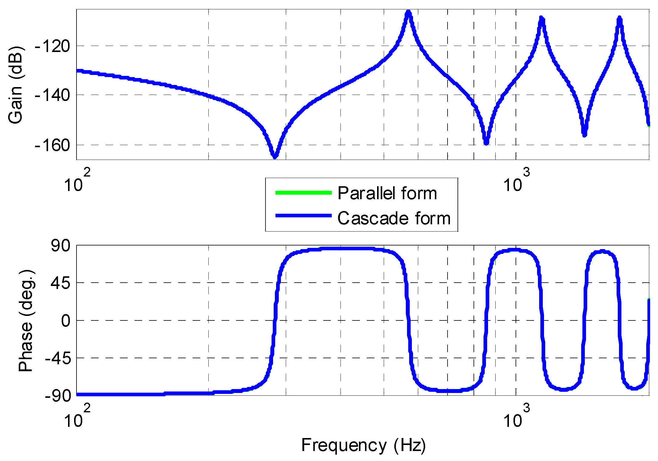
Figure 12 presents the Bode diagrams of the response ${\tilde{H}}_{N,c}\left(j\omega ,s,L\right)$ of the cascade form (in blue) and the response ${\tilde{H}}_{N,p}\left(j\omega ,s,L\right)$ of the parallel form (in green) on the range [100, 2000] Hz, where we observe the perfect superposition of the two curves.

Thus, the procedure presented in this paragraph and illustrated in the nominal case m = 0.5 must be repeated for each value of m considered belonging to the interval [0, 1]. This procedure makes it possible to obtain the rational forms ${\tilde{H}}_{N,c}\left(x,s,L\right)$ and ${\tilde{H}}_{N,p}\left(x,s,L\right)$; the fractional form $\tilde{H}\left(x,s,L\right)$ is necessary for the temporal simulation within the HIL (Hardware in the Loop) simulation platform.

5. Conclusions and Future Works

The structure and progression of this article are organized in a didactic way so that readers with no idea about visco-thermal losses in wind instruments can “absorb” the dynamic behavior of an acoustic tube of constant radius. From the two partial differential equations that define the Webster–Lokshin model, a classical resolution in the operational domain leads to the analytical expression of the acoustic impedance and admittance of the function tube of position x, its length L, and its radius r.

Moreover, a system vision is proposed aiming to causally decompose the global model into sub-models, thus facilitating analysis in the frequency domain. One of the conclusions of this frequency analysis is that the fractional model can be simplified over the range [20–20,000] Hz of the audible frequencies. In addition, the introduction of an uncertainty at the level of the fractional order (whose value considered as nominal is that of the initial Webster–Lokshin model, namely m₀ = 0.5) allows us to study the influence of the order m when this varies between 0 (conservative case) and 1.

As is often the case with fractional models, simulation in the time domain requires the establishment of rational forms. Thus, two rational forms composed of an integrator and N second-order cells, one in cascade and the other in parallel, were introduced. Then, the parameters of the cascade form are determined using the Frequency Domain System Identification (FDSI) module of the CRONE Toolbox. As for the parameters of the parallel form, they are obtained by a decomposition into simple elements of the cascade form.

More generally in the fractional model, this study of visco-thermal losses within the resonator of a wind instrument leads to a finding similar to that already made in other fields. Indeed, the main interest of the fractional form resides in the parametric parsimony, that is to say, the capacity that the integro-differential operator of non-integer order has to model with a minimum of parameters the greatest number dynamic phenomena. Thus, the study of parametric sensitivity, in particular in the frequency domain, is simpler.

As a future work, a comparison between the simulated values and the exact outputs can be computed in order to compare the approximation effects from a practical point of view. Thus, the model uncertainties will be analyzed in more detail when comparing the real and the simulated systems. Added to that, building resonators with the same fractional order as proposed in this article will be a major challenge, as going from simulated systems to implemented ones will be an innovation in the musical instruments field. So, in more detail, an extension of the fractional model to take into account the visco-elastic losses is proposed, thus making it possible to vary the fractional order m from 0 (conservative system) to 1 (very dissipative system), and not to consider only m = 0.5 as is currently the case in the literature. This domain [0; 1] belonging to the order m makes it possible to better account for the influence of geometry (radius r and length L), the roughness, and the nature of the material of the resonator.

References

- Tassart, S. Modélisation, Simulation et Analyse des Instruments à Vent Avec Retards Fractionnaires. Ph.D. Thesis, Université Paris VI, Paris, France, 1999. [Google Scholar]
- Hélie, T. Modélisation physique d’instruments de musique en systèmes dynamiques et inversion. JESA 2003, 37, 1305–1310. [Google Scholar] [CrossRef]
- Hélie, T. Unidimensional models of acoustic propagation in axisymmetric wave guides. J. Acoust. Soc. Am. 2003, 114, 2633–2647. [Google Scholar] [CrossRef] [PubMed]
- Rémi, M.; Thomas, H.; Denis, M. Simulation en guides d’ondes numériques stables pour des tubes acoustiques à profil convexe. J. Eur. Syst. Autom. JESA 2011, 45, 547–574. [Google Scholar]
- Hélie, R.M.D.M.T. Waveguide modeling of lossy flared acoustic pipes: Derivation of Kelly-Lochbaum structure for real-time simulations. In Proceedings of the IEEE Workshop on Applications of Signal Processing to Audio and Acoustics, New Paltz, NY, USA, 21–24 October 2007. [Google Scholar]
- Mignot, R. Réalisation en Guides D’ondes Numériques Stables d’un Modèle Acoustique Réaliste Pour la Simulation en Temps réel D’instruments à Vent. Available online: https://pastel.archives-ouvertes.fr/tel-00456997v2/document (accessed on 19 January 2021).
- Hélie, T. Ondes découplées et ondes progressives pour les problèmes mono-dimensionnels d’acoustique linéaire. In Proceedings of the Congrès Français d’Acoustique, CFA’06, Tours, France, 24–27 April 2006. [Google Scholar]
- Lokshin, A.; Rok, V. Fundamental solutions of the wave equation with retarded time. Dokl. Akad. Nauk SSSR 1978, 239, 1305–1308. [Google Scholar]
- Haddar, H.; Matignon, D.; Hélie, T. A Webster-Lokshin Model for Waves with Viscothermal Losses and Impedance Boundary Conditions: Strong Solutions. Available online: https://0-link-springer-com.brum.beds.ac.uk/chapter/10.1007/978-3-642-55856-6_10 (accessed on 19 January 2021).
- Haddar, H.; Matignon, D. Analyse Théorique et Numérique du Modèle de Webster Lokshin; INRIA: Toulouse, France, 2008. [Google Scholar]
- Matignon, D.; d’Andréa-Novel, B.; Depalle, P.; Oustaloup, A. Viscothermal losses in wind instruments: A non-integer model. In Systems and Networks: Mathematical Theory and Applications; Helmke, U., Mennicken, R., Saurer, J., Eds.; Akademie Verlag: Berlin, Germany, 1994; Volume 79, pp. 789–790. [Google Scholar]
- Matignon, D. Représentation en Variables d’état de Modèles de Guides D’ondes Avec Dérivation Fractionnaire. Ph.D. Thesis, Paris XI University, Paris, France, November 1994. [Google Scholar]
- Haddar, H.; Li, J.; Matignon, D. Efficient solution of a wave equation with fractional-order dissipative terms. J. Comput. Appl. Math. 2010, 234, 2003–2010. [Google Scholar] [CrossRef]
- Mignot, R.; Hélie, T.; Matignon, D. Simulation en guides d’ondes numériques stables pour des tubes acoustiques à profil convexe. JESA 2011, 45, 547–574. [Google Scholar] [CrossRef] [Green Version]
- Lombard, B.; Matignon, D.; le Gorrec, Y. A fractional Burgers equation arising in nonlinear acoustics: Theory and numerics. In Proceedings of the 9eme Symposium IFAC sur les Systèmes de Commande Non Linéaires, Toulouse, France, 28 November 2013. [Google Scholar]
- Vigué, P.; Vergez, C.; Lombard, B.; Cochelin, B. Continuation of periodic solutions for systems with fractional derivatives. Nonlinear Dyn. 2019, 95, 479–493. [Google Scholar] [CrossRef] [Green Version]
- Haidar, G.A.; Daou, R.A.Z.; Moreau, X. Modelling and Identification of the Musicians Blowing Part and the Flute Musical Instrument. In Proceedings of the Fourth International Conference on Advances in Computational Tools for Engineering Applications, Zouk, Lebanon, 3–5 July 2019. [Google Scholar]
- Haidar, G.A.; Moreau, X.; Daou, R.A.Z. Modelling, Implementation and Control of a Wind Musical Instrument. In Proceedings of the 21st IFAC World Congress, Berlin, Germany, 2 October 2020. [Google Scholar]
- Haidar, G.A.; Moreau, X.; Daou, R.A.Z. System Approach for the Frequency Analysis of a Fractional Order Acoustic Tube: Application for the Resonator of the Flute Instrument. In Fractional Order Systems: Mathematics, Design, and Applications for Engineers; Elsevier: Amsterdam, The Netherlands, 2021. [Google Scholar]
- Blanc, F. Production de son par Couplage Écoulement/Résonateur: Étude des Paramètres de Facture des Flûtes par Expérimentations et Simulations Numériques D’écoulements. Available online: https://tel.archives-ouvertes.fr/tel-00476600/document (accessed on 19 January 2021).
- Ducasse, E. Modélisation d’instruments de musique pour la synthèse sonore: Application aux instruments à vent. J. Phys. Colloq. 1990, 51, 837–840. [Google Scholar] [CrossRef]
- Ségoufin, C. Production du son par Interaction Écoulement/Résonateur Acoustique. Available online: http://www.lam.jussieu.fr/Publications/Theses/these-claire-segoufin.pdf (accessed on 19 January 2021).
- Ducasse, E. Modélisation et Simulation dans le Domaine Temporel D’instruments à vent à Anche Simple en Situation de jeu: Méthodes et Modèles. Available online: http://cyberdoc.univ-lemans.fr/theses/2001/2001LEMA1013.pdf (accessed on 19 January 2021).
- Terrien, S. Instrument de la Famille des Flûtes: Analyse des Transitions Entre Régimes. Available online: https://scanr.enseignementsup-recherche.gouv.fr/publication/these2014AIXM4756 (accessed on 19 January 2021).
- Beranek, L. Acoustics; Amer Inst of Physics: Woodbury, NY, USA, 1986. [Google Scholar]
- Chaigne, J.K.A. Acoustique des Instruments de Musique, 2nd ed.; Edition Belin: Paris, France, 2013. [Google Scholar]
- Boutin, H.; le Conte, S.; le Carrou, J.L.; Fabre, B. Modèle de Propagation Acoustique dans un Tuyau Cylindrique à Paroi Poreuse. Available online: https://hal.archives-ouvertes.fr/hal-01830275/ (accessed on 19 January 2021).
- Mignot, R.; Hélie, T.; Matignon, D. From a model of lossy frared pipes to a general framework for simulation of waveguides. Acta Acust. United Acust. 2011, 97, 477–491. [Google Scholar] [CrossRef]
- Hélie, T.; Gandolfi, G.; Hezard, T. Estimation paramétrique de la perce d’un instrument à vent à partir de la mesure de son impédance d’entrée. Available online: https://hal.archives-ouvertes.fr/hal-01106923 (accessed on 19 January 2021).
- Assaf, R. Modélisation des Phénomènes de Diffusion Thermique dans un Milieu fini Homogène en vue de L’analyse, de la Synthèse et de la Validation de Commandes Robustes. Available online: https://hal.archives-ouvertes.fr/tel-01247918 (accessed on 19 January 2021).
- Debut, V. Deux études d’un Instrument de Musique de type Clarinette: Analyse des Fréquences Propres du Résonateur et Calcul des Auto-Oscillations par Décomposition Modale. Ph.D. Thesis, Université Aix-Marseille II, Marseille, France, 2004. [Google Scholar]
- Malti, S.V.R. CRONE Toolbox for system identification using fractional differentiation models. In Proceedings of the 17th IFAC Symposum on System Identification, SYSID’15, Beijing, China, 19–21 October 2015; pp. 769–774. [Google Scholar]
Figure 1.
One-dimensional description of an acoustic tube of radius r = constant and of finite length L subjected to an acoustic flow Qv(t) with x = 0.
Figure 2.
Block diagrams associated with the system approach: whenever x is between 0 and L (a), at x = 0 for the finite system L (b), at x = 0 for a semi finite system (c).
Figure 3.
Bode diagrams of Im(jω) on the range [10−4; 104] Hz.
Figure 4.
Frequency response of Im(jω) on the range [20–20,000] Hz of the audible frequencies.
Figure 5.
Bode diagrams of F(0, jω,L) on the range [10−4; 104] Hz.
Figure 6.
Bode diagrams of 1/F(0,jω,L) (in red) and of T(0,jω,L) (in blue) in the range [10−4; 104] Hz (a) and in the range [20–4000] Hz of audible and achievable frequencies with a recorder (b).
Figure 7.
Bode diagrams in x = 0 (ωL,x/2π = 184 Hz), in x = L/2 (ωL,x/2π = 368 Hz), and in x = 3L/4 (ωL,x/2π = 735 Hz) of x = 3L/4 (ωL,x/2π = 735 Hz) (in black), of H(L/2,jω,L) (in blue), and of H(3L/4,jω,L) (in red) on the beach [20–4000] Hz of audible and achievable.
Figure 8.
Bode diagrams at x = 0 of H(0,jω,L) for different values of the fractional order m on the range [20–4000] Hz of audible and achievable frequencies with a recorder.
Figure 9.
Reduced frequency responses H(0,jω,L)/H0 with the frequency axis on a linear scale over the range [150; 750] Hz.
Figure 10.
Block diagrams associated with the simplified model: whenever x is between 0 and L (a), at x = 0 for the finite system of length L, (b) and at x = 0 for a semi-infinite system (c).
Figure 11.
Screenshots from the CRONE Toolbox before optimization (a) and after optimization (b) at x = 0 in the nominal case m = 0.5.
Figure 12.
Bode diagrams of the response of the cascade form (in blue) and of the response of the parallel form (in green) over the range [100–2000] Hz.