
Local Convergence and Dynamical Analysis of a Third and Fourth Order Class of Equation Solvers

 ,
,  , and
, and
Abstract
:1. Introduction
2. Local Convergence Analysis of the Discussed Family of Iterative Algorithms
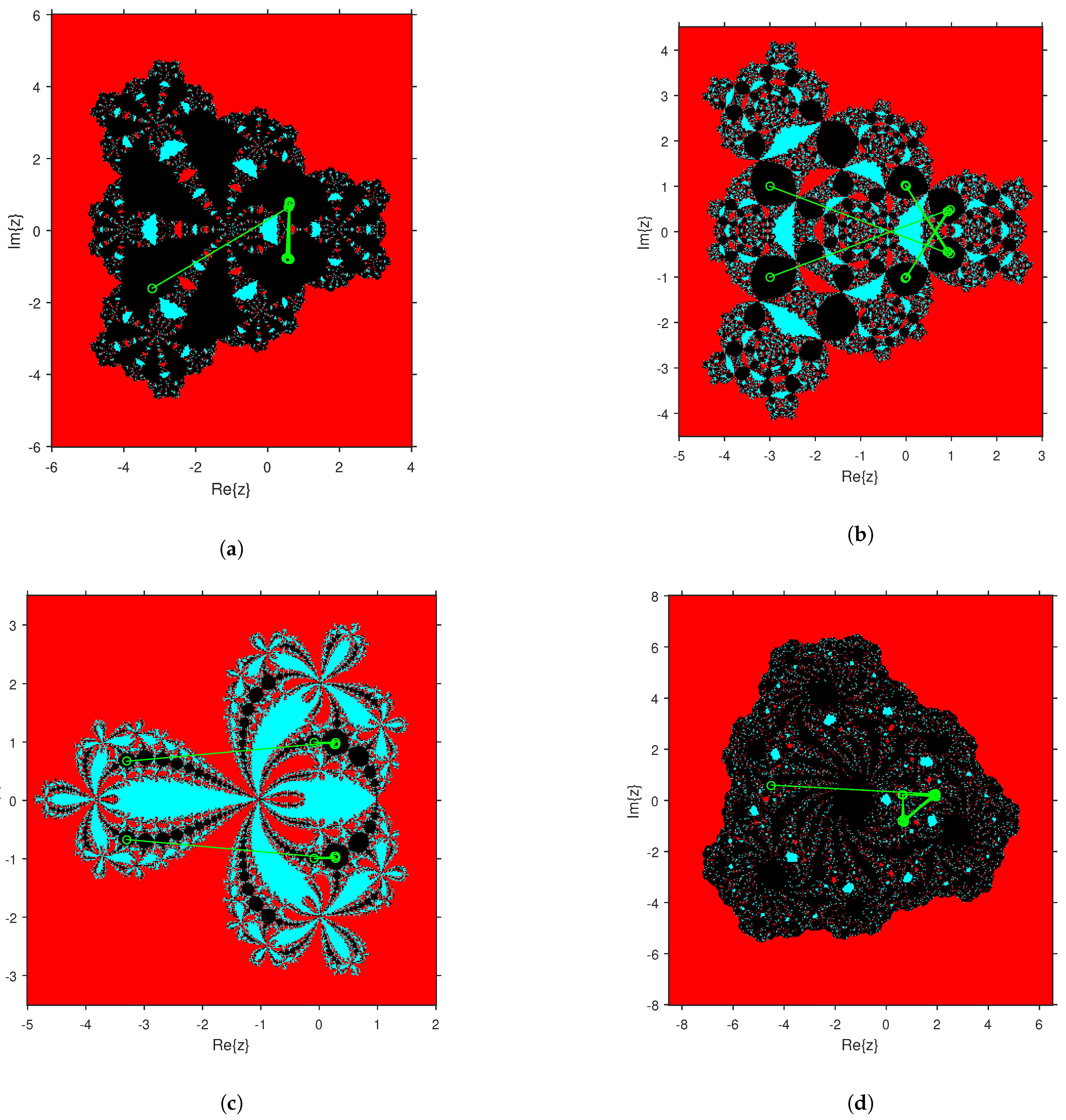
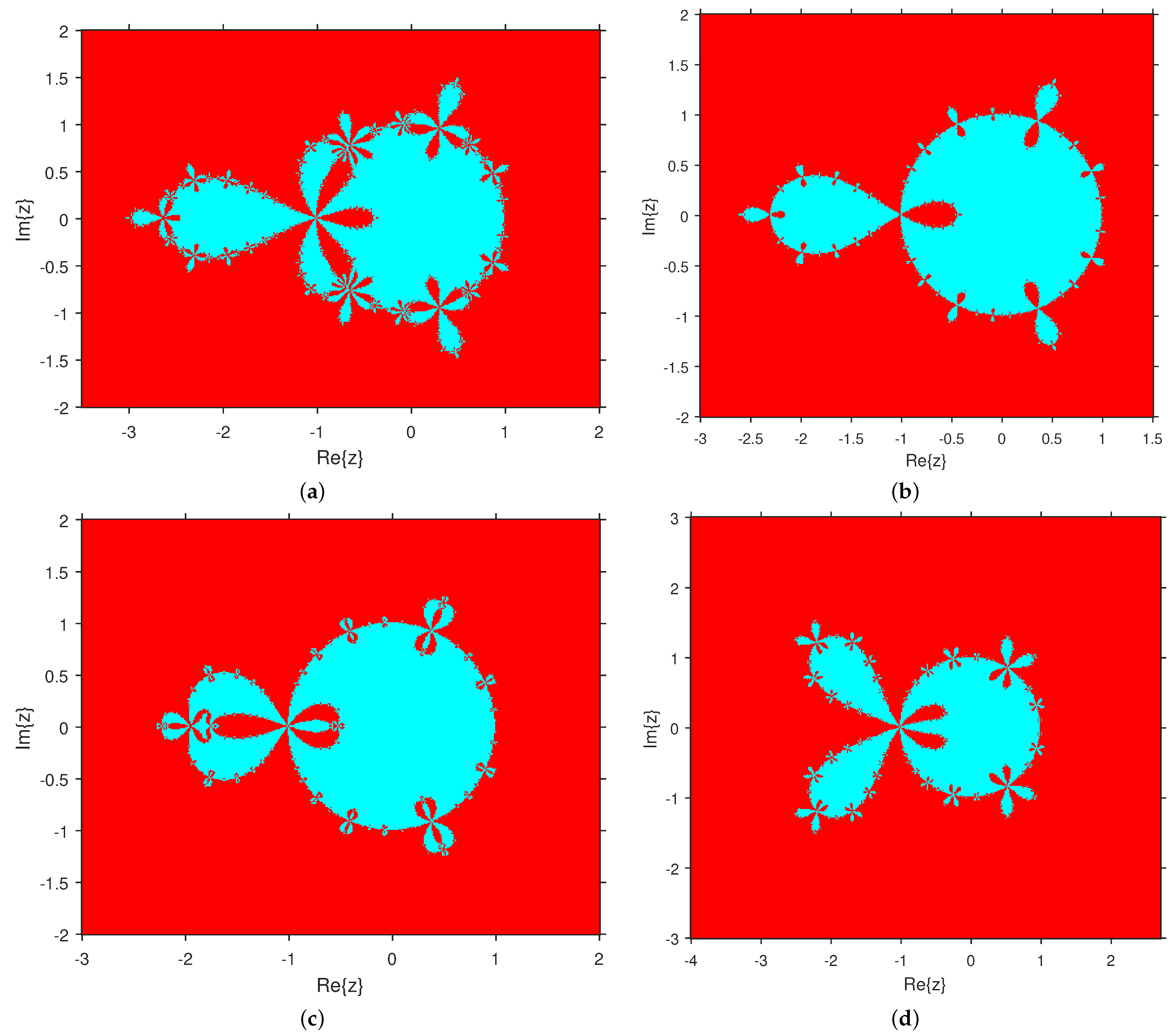
3. Complex Dynamics of the Discussed Class of Methods
3.1. Study of Fixed Points and Their Stability
- 1.
- 2.
- 3.
- 4.
- (i)
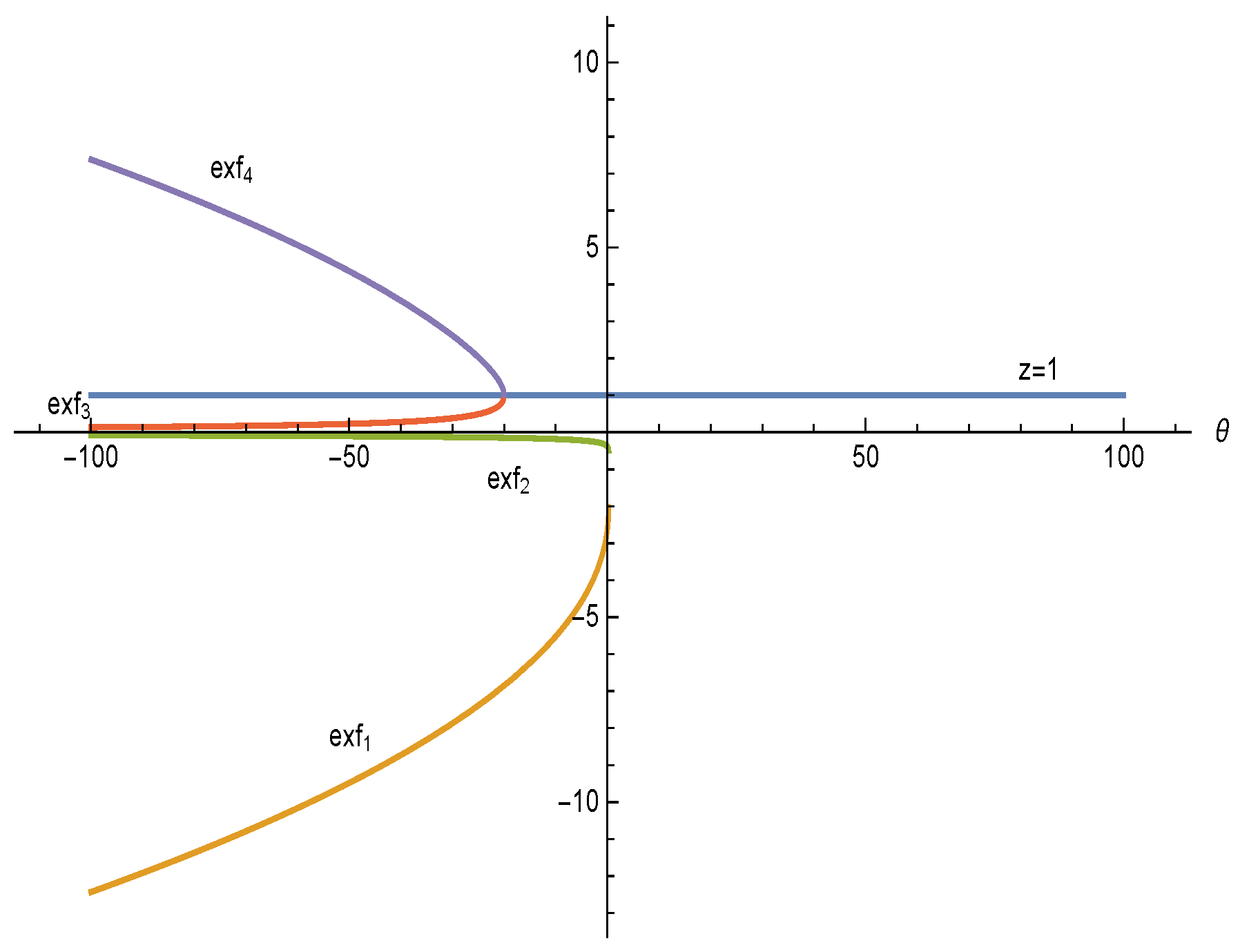
- If , then has three strange fixed points.
- (ii)
- If , then and the number of strange fixed points is three.
- (iii)
- If , then and . Hence the number of strange fixed points of is three.
- 1.
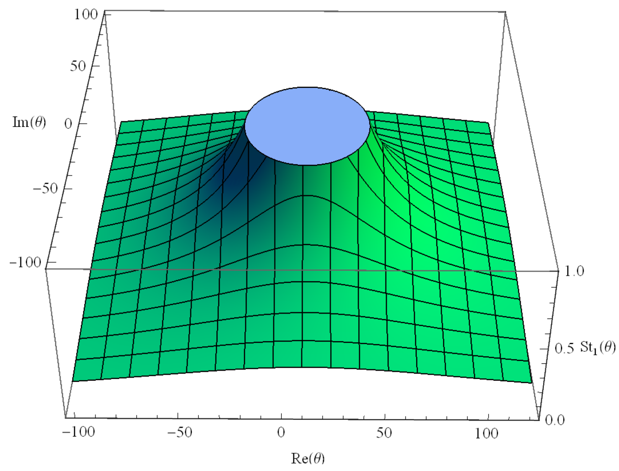
- If , then is attracting. In addition, it cannot be superattracting for any value of θ.
- 2.
- If , then is a parabolic fixed point.
- 3.
- is a repulsor when .
- 1.
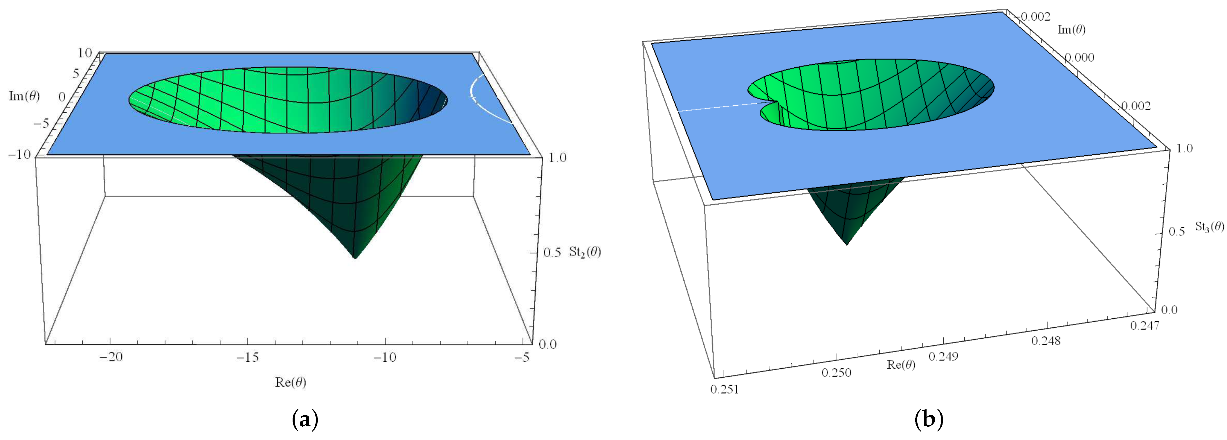
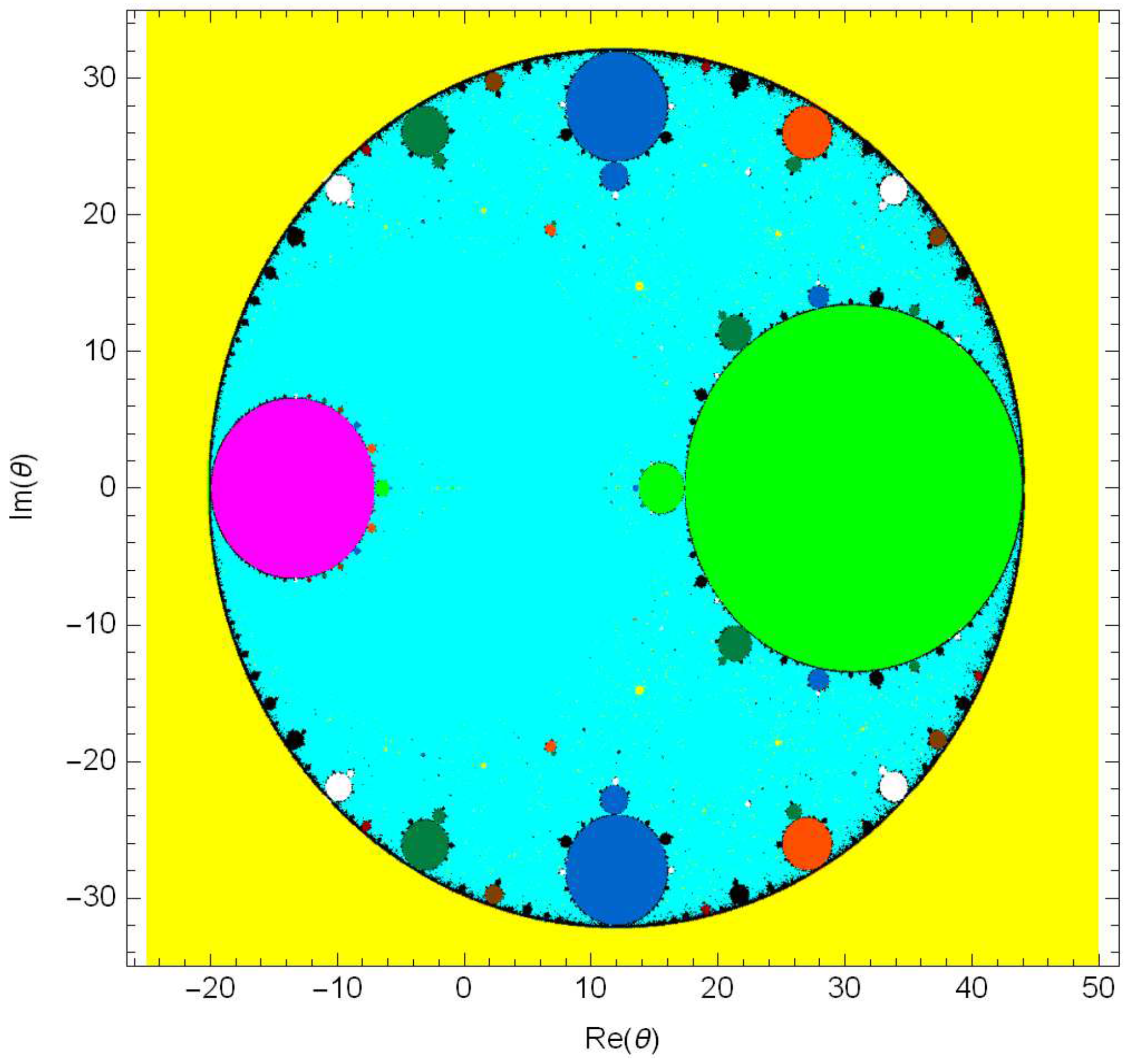
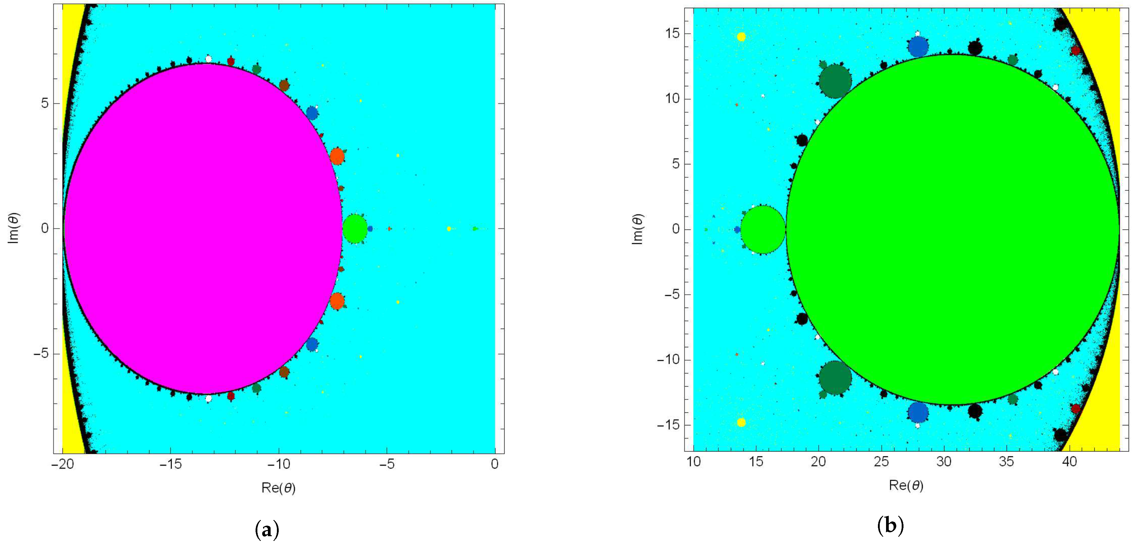
- The stability of and is the same. In detail,* If , then both fixed points are superattractive fixed points.* Additionally, these fixed points are attractors if θ lies in the oval or cardioid presented in Figure 3a,b, respectively.
- 2.
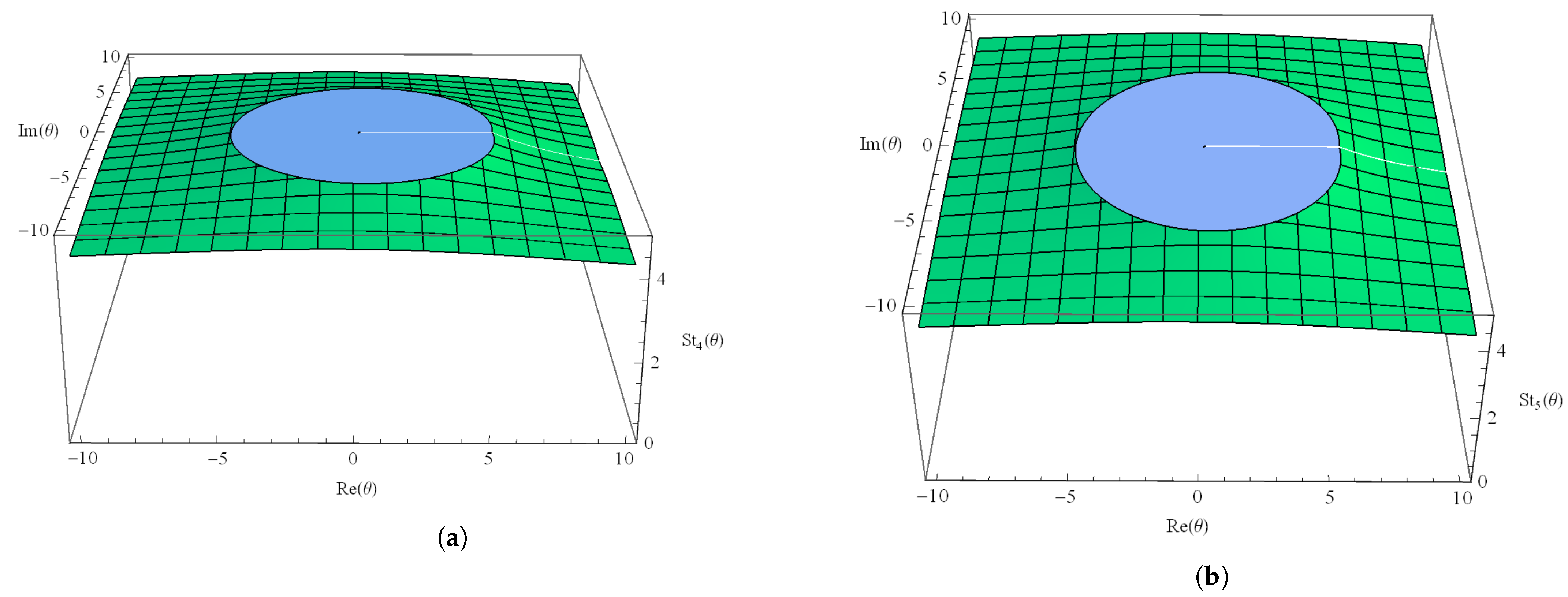
- The fixed points and are always repulsive in nature for any value of θ, and this can be observed in Figure 4a,b, respectively.
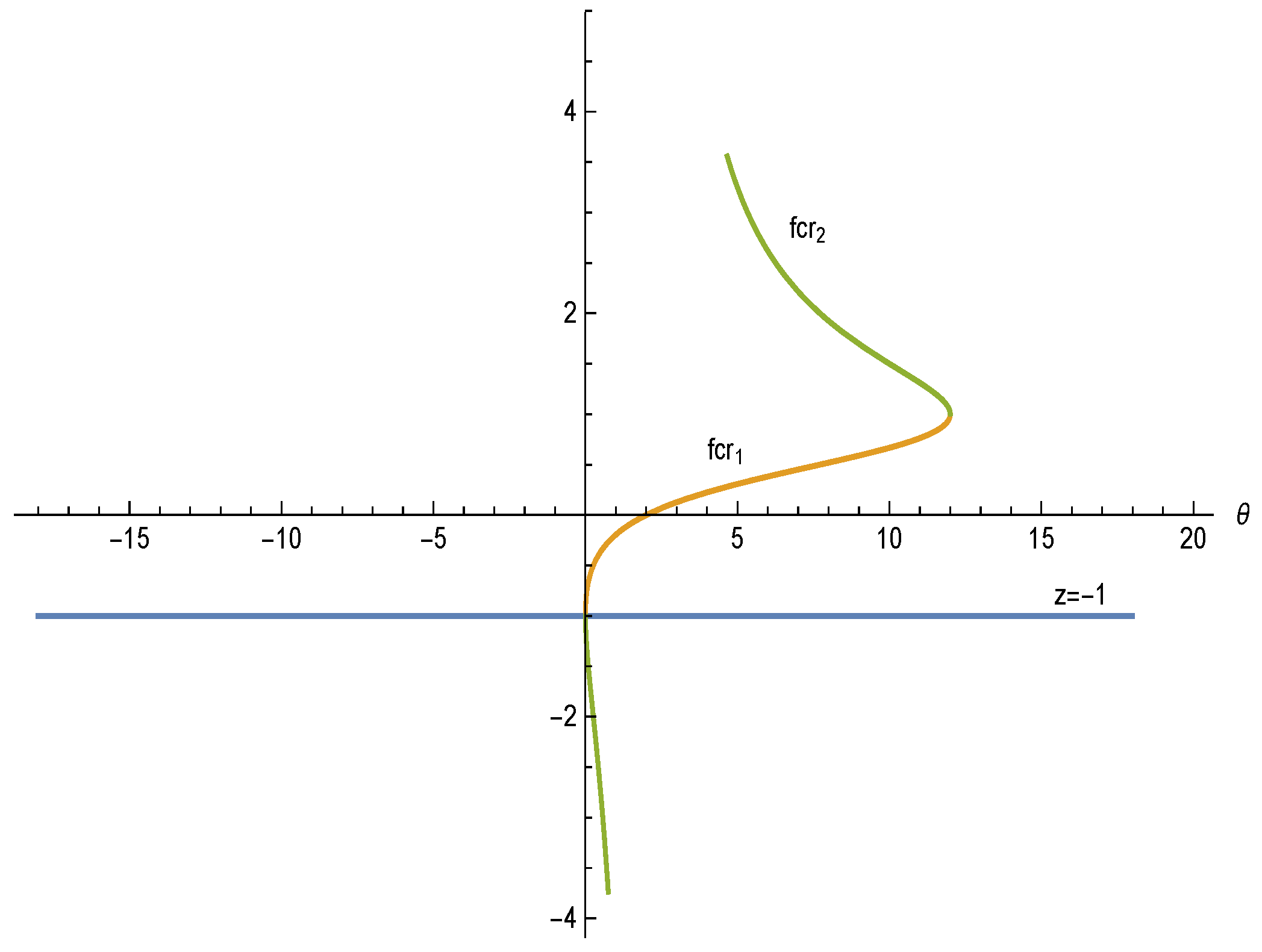
3.2. Study of Critical Points and Parameter Spaces
- 1.
- 2.
- (i)
- If , then the number of distinct free critical points of is one.
- (ii)
- For the rest of scenarios, the operator has three distinct free critical points.
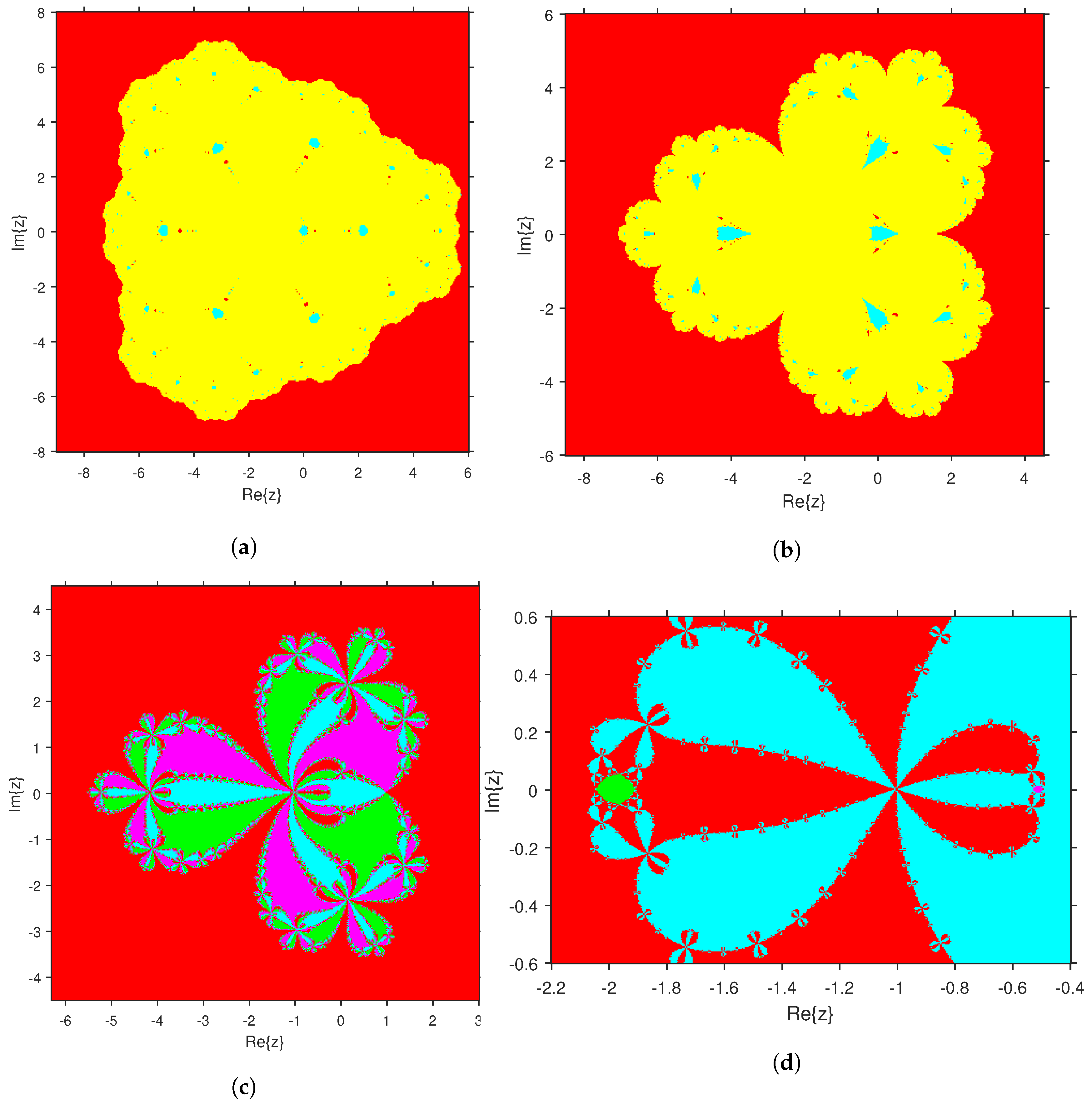
4. Numerical Examples
Author Contributions
Funding
Institutional Review Board Statement
Informed Consent Statement
Data Availability Statement
Conflicts of Interest
References
- Argyros, I.K. Convergence and Application of Newton-Type Iterations; Springer: Berlin/Heidelberg, Germany, 2008. [Google Scholar]
- Argyros, I.K.; Cho, Y.J.; Hilout, S. Numerical Methods for Equations and Its Applications; Taylor & Francis, CRC Press: New York, NY, USA, 2012. [Google Scholar]
- Behl, R.; Cordero, A.; Motsa, S.S.; Torregrosa, J.R.; Kanwar, V. An optimal fourth-order family of methods for multiple roots and its dynamics. Appl. Math. Comput. 2016, 71, 775–796. [Google Scholar] [CrossRef]
- Candela, V.; Marquina, A. Recurrence relations for rational cubic methods I: The Halley method. Computing 1990, 44, 169–184. [Google Scholar] [CrossRef]
- Ezquerro, J.; Hernández, M.A. On Halley-type iteration with free second derivative. J. Comput. Appl. Math. 2004, 170, 455–459. [Google Scholar] [CrossRef] [Green Version]
- Ezquerro, J.A.; González, D.; Hernández, M.A. Majorizing sequences for Newton’s method from initial value problems. J. Comput. Appl. Math. 2012, 2012 236, 2246–2258. [Google Scholar] [CrossRef] [Green Version]
- Grau, M.; Diaz-Barrero, J.L. An improvement of the Euler-Chebyshev iterative method. J. Math. Anal. Appl. 2006, 315, 1–7. [Google Scholar] [CrossRef] [Green Version]
- Kou, J.; Li, Y.; Wang, X. Fourth-order iterative methods free from second derivative. Appl. Math. Comput. 2007, 184, 880–885. [Google Scholar] [CrossRef]
- Maroju, P.; Magreñán, Á.A.; Motsa, S.S.; Sarría, Í. Second derivative free sixth order continuation method for solving nonlinear equations with applications. J. Math. Chem. 2018, 56, 2099–2116. [Google Scholar] [CrossRef]
- Neta, B.; Scott, M.; Chun, C. Basins of attraction for several methods to find simple roots of nonlinear equations. Appl. Math. Comput. 2012, 218, 10548–10556. [Google Scholar] [CrossRef]
- Özban, A.Y. Some new variants of Newton’s method. Appl. Math. Lett. 2004, 17, 677–682. [Google Scholar] [CrossRef] [Green Version]
- Petković, M.S.; Neta, B.; Petković, L.; Dz̃unić, D. Multipoint Methods for Solving Nonlinear Equations; Elsevier: Amsterdam, The Netherlands, 2013. [Google Scholar]
- Rall, L.B. Computational Solution of Nonlinear Operator Equations; Robert E. Krieger: New York, NY, USA, 1979. [Google Scholar]
- Ren, H.; Wu, Q.; Bi, W. New variants of Jarratt method with sixth-order convergence. Numer. Algor. 2009, 52, 585–603. [Google Scholar] [CrossRef]
- Sharma, J.R.; Guna, R.K.; Sharma, R. Efficient Jarratt-like methods for solving systems of nonlinear equations. Calcolo 2014, 51, 193–210. [Google Scholar] [CrossRef]
- Traub, J.F. Iterative Methods for Solution of Equations; Prentice-Hall: Englewood Cliffs, NJ, USA, 1964. [Google Scholar]
- Weerakoon, S.; Fernando, T.G.I. A variant of Newton’s method with accelerated third-order convergence. Appl. Math. Lett. 2000, 13, 87–93. [Google Scholar] [CrossRef]
- Amat, S.; Argyros, I.K.; Busquier, S.; Hernández-Verón, M.A.; Martínez, E. On the local convergence study for an efficient k-step iterative method. J. Comput. Appl. Math. 2018, 343, 753–761. [Google Scholar] [CrossRef]
- Argyros, I.K.; Magreñán, Á.A. On the convergence of an optimal fourth-order family of methods and its dynamics. Appl. Math. Comput. 2015, 252, 336–346. [Google Scholar] [CrossRef]
- Argyros, I.K.; Magreñán, Á.A. A study on the local convergence and the dynamics of Chebyshev-Halley-type methods free from second derivative. Numer. Algor. 2015, 71, 1–23. [Google Scholar] [CrossRef]
- Argyros, I.K.; Cho, Y.J.; George, S. Local convergence for some third order iterative methods under weak conditions. J. Korean Math. Soc. 2016, 53, 781–793. [Google Scholar] [CrossRef] [Green Version]
- Argyros, I.K.; George, S. Local convergence for an almost sixth order method for solving equations under weak conditions. SeMA J. 2017, 75, 163–171. [Google Scholar] [CrossRef]
- Argyros, I.K.; Sharma, D.; Parhi, S.K. On the local convergence of Weerakoon-Fernando method with ω continuity condition in Banach spaces. SeMA J. 2020, 77, 291–304. [Google Scholar] [CrossRef]
- Argyros, I.K.; George, S. On the complexity of extending the convergence region for Traub’s method. J. Complex. 2020, 56, 101423. [Google Scholar] [CrossRef]
- Argyros, I.K.; Behl, R.; González, D.; Motsa, S.S. Ball convergence for combined three-step methods under generalized conditions in Banach space. Stud. Univ. Babes-Bolyai Math. 2020, 65, 127–137. [Google Scholar] [CrossRef]
- Maroju, P.; Magreñán, Á.A.; Sarría, Í.; Kumar, A. Local convergence of fourth and fifth order parametric family of iterative methods in Banach spaces. J. Math. Chem. 2020, 58, 686–705. [Google Scholar] [CrossRef]
- Sharma, D.; Parhi, S.K. Local Convergence and Complex Dynamics of a Uni-parametric Family of Iterative Schemes. Int. J. Appl. Comput. Math. 2020, 6, 1–16. [Google Scholar] [CrossRef]
- Singh, S.; Gupta, D.K.; Badoni, R.P.; Martínez, E.; Hueso, J.L. Local convergence of a parameter based iteration with Hölder continuous derivative in Banach spaces. Calcolo 2017, 54, 527–539. [Google Scholar] [CrossRef]
- Amat, S.; Busquier, S.; Plaza, S. Review of some iterative root-finding methods from a dynamical point of view. Sci. Ser. A Math. Sci. 2004, 10, 3–35. [Google Scholar]
- Amat, S.; Busquier, S.; Plaza, S. Dynamics of the King and Jarratt iterations. Aequationes Math. 2005, 69, 212–223. [Google Scholar] [CrossRef]
- Cordero, A.; García-Maimó, J.; Torregrosa, J.R.; Vassileva, M.P.; Vindel, P. Chaos in King’s iterative family. Appl. Math. Lett. 2013, 26, 842–848. [Google Scholar] [CrossRef] [Green Version]
- Cordero, A.; Torregrosa, J.R.; Vindel, P. Dynamics of a family of Chebyshev-Halley type methods. Appl. Math. Comput. 2013, 219, 8568–8583. [Google Scholar] [CrossRef] [Green Version]
- Cordero, A.; Guasp, L.; Torregrosa, J.R. Choosing the most stable members of Kou’s family of iterative methods. J. Comput. Appl. Math. 2018, 330, 759–769. [Google Scholar] [CrossRef]
- Cordero, A.; Villalba, E.G.; Torregrosa, J.R.; Triguero-Navarro, P. Convergence and Stability of a Parametric Class of Iterative Schemes for Solving Nonlinear Systems. Mathematics 2021, 9, 86. [Google Scholar] [CrossRef]
- Chicharro, F.; Cordero, A.; Gutiérrez, J.M.; Torregrosa, J.R. Complex dynamics of derivative-free methods for nonlinear equations. Appl. Math. Comput. 2013, 2013 219, 7023–7035. [Google Scholar] [CrossRef]
- Chicharro, F.; Cordero, A.; Torregrosa, J.R. Drawing dynamical and parameters planes of iterative families and methods. Sci. World J. 2013, 2013, 780153. [Google Scholar] [CrossRef] [PubMed]
- Magreñán, Á.A. Different anomalies in a Jarratt family of iterative root-finding methods. Appl. Math. Comput. 2014, 233, 29–38. [Google Scholar]


Publisher’s Note: MDPI stays neutral with regard to jurisdictional claims in published maps and institutional affiliations. |
© 2021 by the authors. Licensee MDPI, Basel, Switzerland. This article is an open access article distributed under the terms and conditions of the Creative Commons Attribution (CC BY) license (https://creativecommons.org/licenses/by/4.0/).
Share and Cite
Sharma, D.; Argyros, I.K.; Parhi, S.K.; Sunanda, S.K. Local Convergence and Dynamical Analysis of a Third and Fourth Order Class of Equation Solvers. Fractal Fract. 2021, 5, 27. https://0-doi-org.brum.beds.ac.uk/10.3390/fractalfract5020027
Sharma D, Argyros IK, Parhi SK, Sunanda SK. Local Convergence and Dynamical Analysis of a Third and Fourth Order Class of Equation Solvers. Fractal and Fractional. 2021; 5(2):27. https://0-doi-org.brum.beds.ac.uk/10.3390/fractalfract5020027
Chicago/Turabian StyleSharma, Debasis, Ioannis K. Argyros, Sanjaya Kumar Parhi, and Shanta Kumari Sunanda. 2021. "Local Convergence and Dynamical Analysis of a Third and Fourth Order Class of Equation Solvers" Fractal and Fractional 5, no. 2: 27. https://0-doi-org.brum.beds.ac.uk/10.3390/fractalfract5020027