
Simultaneous Identification of Volatility and Mean-Reverting Parameter for European Option under Fractional CKLS Model

School of Mathematics, Renmin University of China, Beijing 100872, China
*
Author to whom correspondence should be addressed.
Fractal Fract. 2022, 6(7), 344; https://0-doi-org.brum.beds.ac.uk/10.3390/fractalfract6070344
Submission received: 21 May 2022
/
Revised: 13 June 2022
/
Accepted: 14 June 2022
/
Published: 21 June 2022
Abstract
:In this paper, we reconstruct the time-dependent volatility function of the underlying asset and the mean-reverting parameter of the interest rate for European options under the fractional Chan–Karolyi–Longstaff–Sanders (CKLS) stochastic interest rate model. Tikhonov regularization is used to solve the ill-posedness of the inverse problem. The existence and stability of the solution of the regularization problem are given. We employ the alternating direction method of multipliers (ADMM) to iteratively optimize the volatility function and the parameter . Finally, numerical simulations and the empirical analysis are presented to illustrate the efficiency of the proposed method.
1. Introduction
Black-Scholes (B-S) model [1] made a breakthrough in option pricing, which gives the analytic expression of European option based on the Geometric Brownian motion. However, B-S model can not accurately describe the growing option market due to the long-term dependence of the underlying logarithmic returns. Fractional Brownian motion(fBm) was employed to describe it by which was suggested by Mandelbrot and Van Ness [2] as an integral representation of Brownian motion process. If , the increment of fBm has a positive correlation. Furthermore, it has a negative correlation when . Hu and Øskendal [3] applied Wick-It product to give the analytic expression of European option under the fBm framework. Necula [4] gave a risk-neutral valuation theorem when the underlying is driven by fBm . Huang et al. [5] deduced the analytic formula of European option for the fractional Vasicek stochastic interest rate model.
The short-term riskless interest rate is one of the most basic and vital parameters in the financial market. A lot of models have been proposed to interpret its behavior such as Vasicek model [6], Cox–Ingersoll–Ross (CIR) model [7], Constant Elasticity of Variance (CEV) model [8] and so on. Chan et al. [9] popularized the above models to the Chan–Karolyi–Longstaff–Sanders (CKLS) model as
Note that Equation (1) transforms to Vasicek model and CIR model when and , respectively. Both models are widely used in market due to their analytical properties. However, for the general parameter except for (Vasicek), (CIR) and [10], the explict expression for the bond price is hard to obtain. Thus, some methods have been developed for the approximation to the closed form solution such as Monte Carlo simulations [11], the analytical approximation formula [12,13,14] and numerical solutions of the corresponding partial differential Equation (PDE) [15,16]. Mao et al. [17] considered the Euler–Maruyama (EM) scheme for the typical hybrid mean-reverting -process and the convergence of EM solution when . Wu et al. [18] gave the analytical properties and the convergence of numerical solutions in probability with . As for the fractional CKLS model, Marie [19] discussed the local existence of solution in rough paths sense. Kubilius and [20] found the sufficiently simple conditions when the solution of fractional CKLS for and is positive, and obtained the convergence rate of the backward Euler approximation method for solutions of fractional CKLS model.
Volatility describes the randomness of the underlying asset price, it can efficaciously reduce the risks caused by market prices fluctuations but it can not be observed directly in market. Thus, there are many researches estimating volatility function from market data [21,22,23]. On the other hand, the parameter controls the relationship between the volatility of interest changes and the level of rate. Therefore, the reconstruction of the volatility and parameter from market data is practical to financial market. Cristofol and Roques [24] showed that the nonlinear drift and diffusion coefficients are simultaneously uniquely determined by the observation of the expectation and variance of a one-dimensional diffusion process, and solved the corresponding inverse problem with PDE technics mainly by the strong parabolic maximum principle.
Regularization is a practical tool to treat the ill-posedness occurred in the inverse problem. Naumova and Pereverzyev [25] proposed a multi-penalty regularization with a component-wise penalization and exhibited the compensatory property of the regularized approximation. Hofmann et al. [26] used a two-parameter Tikhonov regularization with heuristic parameter choice rules to settle the ill-posed nonlinear inverse problem which is the simultaneous recovery of implied volatility and interest rate functions from market data. Georgiev and Vulkov [27] considered an algorithm of predictor-corrector type to recover the piecewise linear time-dependent volatility and risk-free interest rate functions. In this paper, we try to reconstruct the volatility function and parameter from market option prices by alternating direction method of multiplier (ADMM) and Euler–Lagrange iterative method [22], then present the empirical analysis of Shanghai Stock Exchange (SSE) 50ETF.
The rest of this paper is organized as follows. In Section 2, we give the PDE for European option pricing under the fractional CKLS stochastic interest rate model. Section 3 introduces the Tikhonov regularization and gives the existence and stability of the regularized problem, and presents the ADMM algorithm which is used to iteratively optimize the volatility and parameter . The numerical verification is demonstrated in Section 4 with synthetic and real market data. Finally, some conclusions are stated in Section 5.
2. Problem Formulation
In this section, we consider the fractional CKLS model and derive the PDE for pricing the European option. Let S and r be the underlying asset price and stochastic interest rate, respectively. Their dynamics can be expressed as follows
where H is the Hurst parameter and , are two correlated fractional Brown motions with . is the volatility. are constants. implies the mean-reverting -process.
Firstly we discuss the PDE of zero coupon pricing. Assume that we have a zero coupon bond whose value is given by . Construct an imaginary portfolio consisting of one bond that matures at time and a number of () of the bond which expires at as follows
Using the fractional ’s Lemma, we get the following formula in a small time interval
To eliminate the random term in (3), let
The no-arbitrage condition says that
which implies that
Note that
from (5), and can be set as the following form
where is the introducing market price of risk. Then
with the condition as
Lemma 1.
Suppose that the underlying asset S and the interest rate r follow (2), then the European call option with strike K and maturity T satisfies the PDE
conditional to
Proof.
Construct an imaginary portfolio with one option , a number of () of the underlying asset S and () number of the zero coupon bond as follows
Using the fractional ’s Lemma in a small time , we have
To make this portfolio riskless over the time interval , we choose
in (4), then combine the Formula (7)
Using the no-arbitrage pricing principle (4) gives
□
Direct problem: To solve the option pricing problem (9) and (10), we set the boundary conditions as in [28]:
The boundary condition at can be obtained by setting in Equation (9) which leads to the dynamical boundary
We reverse the time as which means the residual time to maturity. Equation (9) becomes a forward PDE, the terminal condition (10) transforms to an initial term, and the conditions (14) and (15) remain the same. Thus, we get that
with the condition
Then the European call option price can be uniquely determined by the initial and boundary problem as soon as the volatility and parameter are accessible. Furthermore, we apply an implicit finite difference method to numerically solve it.
Calibration problem: Assume that the option prices with maturities and strike prices in market are given. Market calibration requires us to find a volatility function and a parameter which make the recalculated option price satisfy
where and represent the bid and ask price in market, respectively. To accord with (18), we employ the available data to minimize the following error function
where , and is the numerical solution of (16) and (17) with the recovered volatility and parameter .
The option data in market is not sufficient to determine the volatility and uniquely, and the minimum value of the optimization problem (19) depends on market data discontinuously, so the calibration problem is ill-posed. Regularization technique is practical to solve the ill-posedness generally.
3. Problem Regularization
In this section, we consider the Tikhonov regularization method and derive the existence and stability of the solution of the regularized problem.
To obtain the stable solution, we calibrate volatility function and by solving the following minimization problem
where and , is the market data and is the regularization parameter.
3.1. Existence and Stability of the Solutions of the Minimization Problem
Now we discuss the existence and stability results of solutions for the minimization problem. Denote and
for any vector of option prices. In what follows, stands for a function .
Theorem 1
(Existence). Let be fixed and the same as in problem (20). Put
Assume that for some the set is bounded and is weakly lower semi-continuous. Then problem (20) has at least one solution which belongs to .
Proof.
There exists a minimizing sequence since . is a Hilbert space. Every Hilbert space is a reflexive Banach space. In the reflexive Banach space every bounded sequence contains a weakly convergent subsequence. Therefore, contains subsequence weakly tending to some . By weak lower semi-continuity of ,
and by the same weak lower semi-continuity is weakly closed. Therefore, is the minimizer contained in . □
The following theorem is a direct consequence of Theorem 1.
Theorem 2
(Stability). Let and be the same as in Theorem 1 and let assumptions stated there hold. Let further be such that:
(1) ;
(2) ;
(3) is bounded and is weakly lower semi-continuous;
(4) .
Finally, assume that is bounded as well. Then one can extract weakly convergent subsequence such that its limit is the solution of problem (20).
3.2. ADMM Algorithm for the Regularized Problem
The augmented Lagrangian for the above optimization problem (20) is
where is the Lagrange multiplier and is the penalty parameter.
We can divide the minimization problem (21) into two sub-problems as
The iteration process of is
where is the step size. The Lagrange multiplier update commonly uses a step size equal to the penalty parameter [29]. In order to improve the convergence in practice and reduce the dependence on the initial selection of the penalty parameter, a simple scheme of varying penalty parameter such as (3.13) in [29] usually works well. For simplicity, we choose the same step size as the penalty parameter here.
For the sub-problem
Rewrite the right hand side of (24) as an integral that is
where is the Dirac delta function.
Since the above scheme only consider the appointed time , the recovered volatility can not be well applied in the future [22]. So we can employ the historical data to get the calibrated results as
where represents the current time.
Let
and apply the Euler–Lagrange equation to , then
The term need to be calculated and its definition is
We can evaluate the variational derivative by solving a PDE with a similar form to (16). Now consider the partial differential operator as
where I is the identity operator.
The option price V with a disturbed volatility satisfies the following PDE
where is the Dirac delta function. Then differentiating the formula (31) with respect to and estimating its value at , we get
To solve Equation (28) numerically, we can introduce a ’false’ time parameter to make the iteration smoother [30] as follows
where
For the sub-problem of
then minimize the objective function (34) by Particle Swarm optimization (PSO) algorithm.
As for the convergence of the solutions generated by ADMM algorithm, we can similarly deduce it according to Theorem 1 in [23].
4. Computational Experiments
4.1. Numerical Simulation
Here we consider the numerical examples. Let , , then , , the initial value , , the parameters in the interest rate model are
Example 1.
Reconstruct the volatility function in and by
The values of regularization parameter and Lagrange multiplier are . The iteration stop criterion is and the maximum number of iterations is 200, where presents the recovered volatility in the dth iteration. Table 1 gives the true European call option price by Lemma 1 with (35). Figure 1 shows the comparison between the recovered and exact volatility. The recovered value of parameter γ is 1.327. A common measure (absolute error) is used to evaluate the volatility of the iterative algorithm for γ in Table 2 when . It is clear that our algorithm is able to satisfactorily reconstruct volatility function and γ.
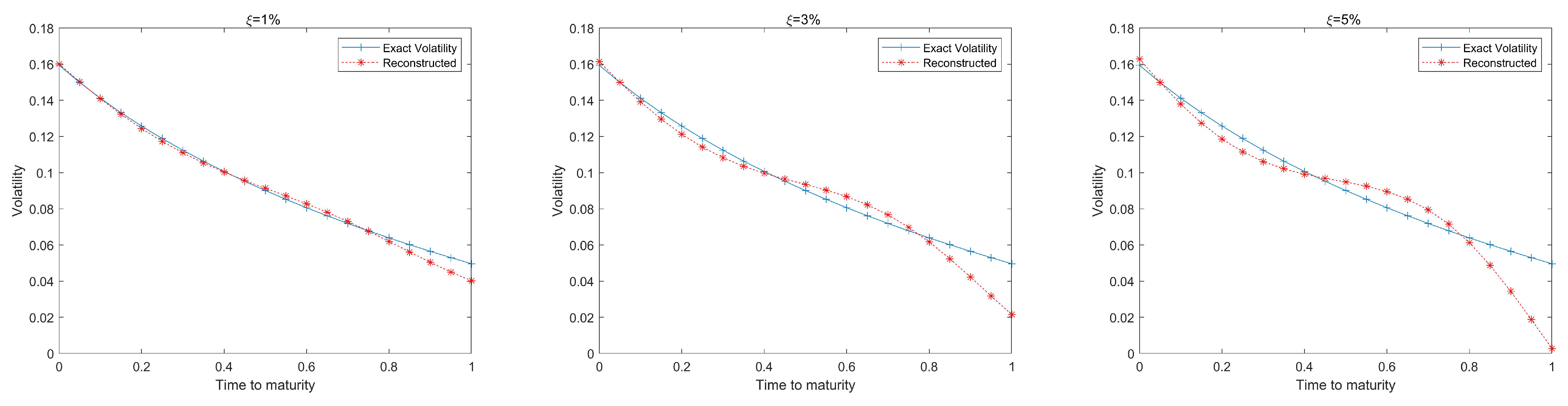
To illustrate the stability of our algorithm, we add the noise with intensity ξ of 1%, 3% and 5% to the exact volatility function (35)
where presents the random number uniformly distributed in the interval (−1,1). Using the noised option prices generated by the disturbed volatility , we can calibrate the volatility and parameter γ again. Figure 2 plots the reconstructed volatility from the noised option prices along with the exact volatility. The recovered parameter γ is 1.171, 1.028 and 0.9512 for the noised cases of 1%, 3% and 5% respectively. Table 2 gives the RMSE and maximum absolute error of recovered volatility and the absolute errors results of γ. Furthermore, the situation of represents the calibration results without noise. We can see that the recovered results are not very accurate, but they can illustrate the stability of our scheme since they are closely located around the exact values.
Example 2.
Recover the in and by
This volatility function shows a ’smile’ curve. We choose the parameters as .
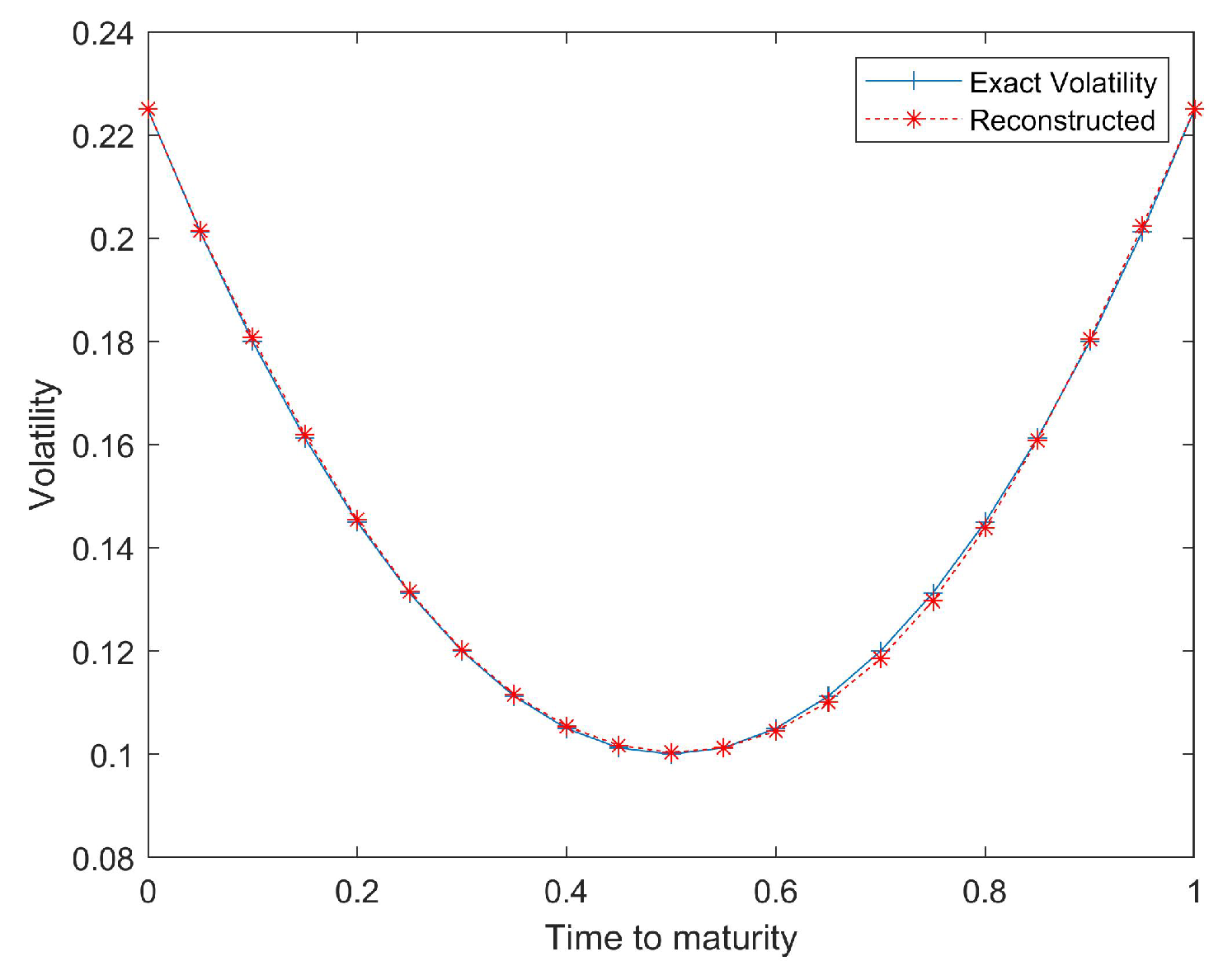
Figure 3 plots the recovered volatility function against the exact one. Table 2 presents the calibrated results for volatility. Root mean square error(RMSE) is used to judge the accuracy of reconstructed volatility with exact volatility as
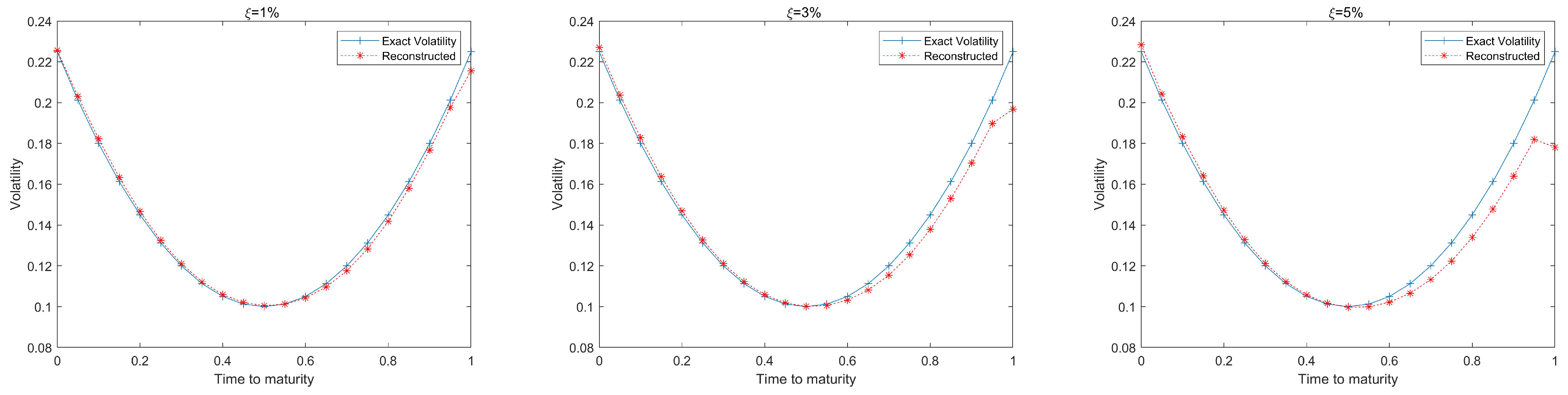
The recovered parameter γ is 0.8020 and its is shown in Table 3. We can see that the proposed scheme can effectively reconstruct the volatility function in the error of . The absolute error of γ is in the . Similarly, we add a little disturbance with the intensity ξ of 1%, 3% and 5% to the exact volatility function (36). Figure 4 plots the reconstructed volatility from the noised option prices along with the noised volatility and the exact one. The recovered parameter γ is 0.811, 0.754 and 0.712 for the noised cases of 1%, 3% and 5% respectively. Table 3 gives the RMSE and maximum absolute error of recovered volatility and the absolute errors results of γ. As expected, the reconstructed volatility and γ from the noised option prices no longer fit very well to the true values due to the disturbance. However, the numerical results also imply the stability of our method as the reconstructed values are close to the exact ones.
4.2. Empirical Analysis
In this part, we try to recover the volatility and parameter from the market data of Shanghai Stock Exchange(SSE) 50ETF on 9 September 2021 [23]. The current price of the underlying asset is , the times to expiration are , the initial interest rate is selected according to Shanghai Inter Bank offered Rate (SHIBOR) 1M at 9 September. The regularization and ADMM parameters are chosen as
Other parameters in our model are chosen by PSO algorithm as
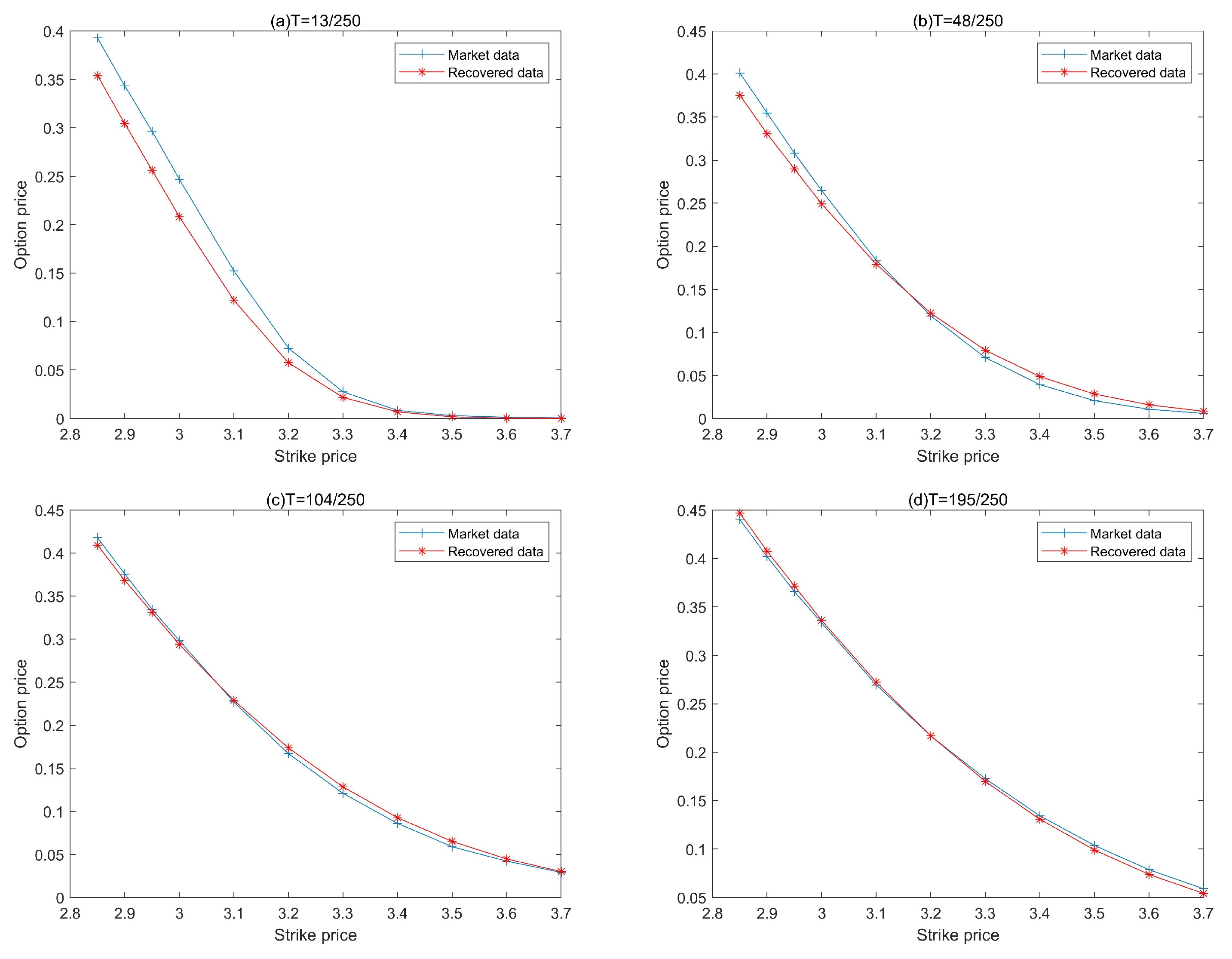
The market data shown in Table 4 is subdivided by cubic spline interpolation to improve the calibration accuracy. The RMSE between the recovered option prices and market prices is used to evaluate the precision of reconstruction results. Table 5 presents the RMSE and maximum absolute error of recalculated option prices, and gives the value of recovered parameter . Figure 5 and Figure 6 specifically report the calibration results. Compared with Table 6 in the empirical analysis of [23], we can see that the recalculated option prices with are more accurate than the Vasicek model. It is clear that the recovered prices at are lower than the market value from Figure 6 due to the interpolation error.
Through the numerical simulation with two typical kinds of volatility functions and the empirical analysis for SSE 50ETF, we conclude that our method is effective and stable to recover the volatility function and parameter simultaneously. Furthermore, it has the potential to be applied in real market.
5. Conclusions
In this paper, we discuss the Tikhonov regularization for the simultaneous recovery of volatility function and mean-reverting parameter from a finite set of market observations by the fractional CKLS model. Firstly we introduce the direct and inverse problems in option market, respectively. Then Tikhonov regularization and ADMM algorithm are applied to solve the ill-posed calibration problem. Finally, several examples are given to demonstrate the accuracy and robustness of our method. Furthermore, empirical analysis implies that the fractional CKLS model with is more suitable than fractional Vasicek model for SSE 50ETF.
Author Contributions
J.Z.: conceptualization, methodology, software, validation, writing—original draft preparation, writing—review and editing; Z.X.: conceptualization, methodology, funding acquisition, supervision, writing—review and editing. All authors have read and agreed to the published version of the manuscript.
Funding
The work was supported by the National Natural Science Foundation of China (Grant No. 12071479).
Acknowledgments
The authors thank the referees for their comments and detailed suggestions. These have significantly improved the presentation of this paper.
Conflicts of Interest
The authors declare no conflict of interest.
References
- Black, F.; Scholes, M. The pricing of option and corporate liabilities. J. Polit. Econ. 1973, 81, 637–654. [Google Scholar] [CrossRef] [Green Version]
- Mandelbrot, B.B.; Ness, J. Fractional brownian motions, fractional noises and applications. SIAM Rev. 1968, 10, 422–437. [Google Scholar] [CrossRef]
- Hu, Y.Z.; Øksendal, B. Fractional white noise calculus and applications to finance. Infin. Dimens. Anal. Quantum Probab. Relat. Top. 2003, 6, 1–32. [Google Scholar] [CrossRef]
- Necula, C. Option pricing in a fractional Brownian motion environment. Adv. Econ. Financ.-Res.—Dofin Work. Pap. Ser. 2008, 2, 259–273. [Google Scholar] [CrossRef]
- Huang, W.L.; Tao, X.X.; Li, S.H. Pricing Formulae for European Options under the Fractional Vasicek Interest Rate Model. Acta Math. Sin. 2012, 55, 219–230. [Google Scholar]
- Vasicek, O.A. An Equilibrium Characterization of the Term Structure. J. Financ. Econ. 1977, 5, 177–188. [Google Scholar] [CrossRef]
- Cox, J.C.; Ingersoll, J.E.; Ross, S.A. A theory of the term structure of interest rates. Econometrica 1985, 53, 385–407. [Google Scholar] [CrossRef]
- Cox, J.C. The constant elasticity of variance option pricing model. J. Portf. Manag. 1996, 23, 15–17. [Google Scholar] [CrossRef]
- Chan, K.C.; Karolyi, G.A.; Longstaff, F.A.; Sanders, A.B. An empirical comparison of alternative models of the short term interest rate. J. Financ. 1992, 47, 1209–1227. [Google Scholar] [CrossRef]
- Brennan, M.J.; Schwartz, E.S. Analyzing convertible bonds. J. Financ. Quant. Anal. 1980, 15, 907–929. [Google Scholar] [CrossRef]
- Glasserman, P. Monte Carlo Methods in Financial Engineering; Springer: Berlin, Germany, 2013. [Google Scholar]
- Choi, Y.; Wirjanto, T.S. An analytic approximation formula for pricing zero-coupon bonds. Financ. Res. Lett. 2007, 4, 116–126. [Google Scholar] [CrossRef]
- Stehlíková, B. A simple analytic approximation formula for the bond price in the Chan-Karolyi-Longstaff-Sanders model. Int. J. Numer. Anal. Model. Ser. B 2013, 4, 224–234. [Google Scholar]
- Stehlíková, B.; Ševcovič, D. Approximate formulae for pricing zero-coupon bonds and their asymptotic analysis. Int. J. Numer. Anal. Model. 2009, 6, 274–283. [Google Scholar]
- Nowman, K.B.; Sorwar, G. Pricing UK and US securities within the CKLS model Further results. Int. Rev. Financ. Anal. 1999, 8, 235–245. [Google Scholar] [CrossRef]
- Nowman, K.B.; Sorwar, G. Derivative prices from interest rate models: Results for Canada, Hong Kong, and United States. Int. Rev. Financ. Anal. 2005, 14, 428–438. [Google Scholar] [CrossRef]
- Mao, X.R.; Truman, A.; Yuan, C. Euler–Maruyama approximations in mean-reverting stochastic volatility model under regime-switching. J. Appl. Math. Stoch. Anal. 2006, 7, 1–20. [Google Scholar] [CrossRef]
- Wu, F.K.; Mao, X.R.; Chen, K. A highly sensitive mean-reverting process in finance and the Euler–Maruyama approximations. J. Math. Anal. Appl. 2008, 348, 540–554. [Google Scholar] [CrossRef] [Green Version]
- Marie, N. A generalized mean-reverting equation and applications. ESAIM Probab. Stat. 2014, 18, 799–828. [Google Scholar] [CrossRef] [Green Version]
- Kubilius, K.; Medžiūnas, A. Positive solutions of the fractional SDEs with fon-lipschitz diffusion coefficient. Mathematics 2021, 9, 18. [Google Scholar] [CrossRef]
- Jiang, L.S.; Tao, Y.S. Identifying the volatility of underlying assets from option prices. Inverse Probl. 2001, 17, 137–155. [Google Scholar]
- Xu, Z.L.; Jia, X.Y. The calibration of volatility for option pricing models with jump diffusion processes. Appl. Anal. 2019, 98, 810–827. [Google Scholar] [CrossRef]
- Zhao, J.J.; Xu, Z.L. Calibration of time-dependent volatility for European options under the fractional Vasicek model. AIMS Math. 2022, 7, 11053–11069. [Google Scholar] [CrossRef]
- Cristofol, M.; Roques, L. Simultaneous determination of the drift and diffusion coefficients in stochastic differential equations. Inverse Probl. 2017, 33, 095006. [Google Scholar] [CrossRef] [Green Version]
- Naumova, V.; Pereverzyev, S.V. Multi-penalty regularization with a component-wise penalization. Inverse Probl. 2013, 29, 075002. [Google Scholar] [CrossRef]
- Hofmann, C.; Hofmann, B.; Pichler, A. Simultaneous identification of volatility and interest rate functions-a two-parameter regularization approach. Electron. Trans. Numer. Anal. 2019, 51, 99–117. [Google Scholar] [CrossRef]
- Georgiev, S.G.; Vulkov, L.G. Simultaneous identification of time-dependent volatility and interest rate for European options. Electron. Trans. Numer. Anal. 2020, 2333, 1–8. [Google Scholar] [CrossRef]
- Haentjens, T.; Hout, K. ADI finite difference schemes for the Heston-Hull-White PDE. J. Comput. Financ. 2012, 16, 83–110. [Google Scholar] [CrossRef]
- Boyd, S.; Parikh, N.; Chu, E.; Peleato, B.; Eckstein, J. Distributed Optimization and Statistical Learning via the Alternating Direction Method of Multipliers. Now Found. Trends 2010, 3, 1–122. [Google Scholar]
- Lagnado, R.; Osher, S. A technique for calibrating derivative security pricing models: Numerical solution of an inverse problem. J. Comput. Financ. 1997, 1, 13–25. [Google Scholar] [CrossRef]
Figure 1.
Comparison between the recovered and exact volatility for Example 1.

Figure 2.
Recovered volatility function against exact one with noise.

Figure 3.
Comparison between the recovered and exact volatility for Example 2.

Figure 4.
Recovered volatility function against exact one for Example 2.

Figure 5.
Left: Market prices; Right: Recovered prices.

Figure 6.
Comparison of SSE 50ETF option price with recovered prices.


Table 1.
The exact option prices for Example 1.
| K | 64 | 68 | 72 | 76 | 80 |
|---|---|---|---|---|---|
| 1.4032 | 0.4094 | 0.0917 | 0.0165 | 0.0025 | |
| 2.5149 | 1.1465 | 0.4555 | 0.1600 | 0.0506 |
Table 2.
The numerical results of recovered and .
| RMSE | AE | ||||
|---|---|---|---|---|---|
| 1.9305 × 10 | 5.7762 × 10 | 1.0623 × 10 | 1.327 | 0.0056 | |
| 3.8220 × 10 | 3.0564 × 10 | 9.3685 × 10 | 1.171 | 0.1504 | |
| 7.7861 × 10 | 8.1093 × 10 | 2.8106 × 10 | 1.028 | 0.2934 | |
| 1.2144 × 10 | 1.1219 × 10 | 4.6803 × 10 | 0.9512 | 0.3702 |
Table 3.
The numerical results of recovered and .
| RMSE | AE | ||||
|---|---|---|---|---|---|
| 7.7267 × 10 | 7.7984 × 10 | 1.6680 × 10 | 0.802 | 0.002 | |
| 7.6843 × 10 | 9.3685 × 10 | 2.1668 × 10 | 0.811 | 0.011 | |
| 7.5211 × 10 | 5.2394 × 10 | 2.8106 × 10 | 0.754 | 0.046 | |
| 7.4837 × 10 | 8.4450 × 10 | 4.6843 × 10 | 0.712 | 0.088 |
Table 4.
The SSE 50ETF option price at 9 September 2021.
| Strike Price K | ||||
|---|---|---|---|---|
| 2.85 | 0.3928 | 0.4013 | 0.4179 | 0.4401 |
| 2.90 | 0.3434 | 0.3548 | 0.3758 | 0.4019 |
| 2.95 | 0.2966 | 0.3082 | 0.3347 | 0.3659 |
| 3.00 | 0.2470 | 0.2647 | 0.2984 | 0.3334 |
| 3.10 | 0.1523 | 0.1837 | 0.2269 | 0.2695 |
| 3.20 | 0.0726 | 0.1192 | 0.1671 | 0.2167 |
| 3.30 | 0.0275 | 0.0707 | 0.1210 | 0.1727 |
| 3.40 | 0.0084 | 0.0393 | 0.0860 | 0.1343 |
| 3.50 | 0.0030 | 0.0207 | 0.0590 | 0.1038 |
| 3.60 | 0.0014 | 0.0107 | 0.0422 | 0.0787 |
| 3.70 | 0.0008 | 0.0059 | 0.0290 | 0.0591 |
Table 5.
The calibration results for SSE 50ETF option.
| RMSE | ||||
|---|---|---|---|---|
| Empirical results | 4.99 × 10 | 0.0151 | 0.0402 | 0.8451 |
Publisher’s Note: MDPI stays neutral with regard to jurisdictional claims in published maps and institutional affiliations. |
© 2022 by the authors. Licensee MDPI, Basel, Switzerland. This article is an open access article distributed under the terms and conditions of the Creative Commons Attribution (CC BY) license (https://creativecommons.org/licenses/by/4.0/).
Share and Cite
MDPI and ACS Style
Zhao, J.; Xu, Z. Simultaneous Identification of Volatility and Mean-Reverting Parameter for European Option under Fractional CKLS Model. Fractal Fract. 2022, 6, 344. https://0-doi-org.brum.beds.ac.uk/10.3390/fractalfract6070344
AMA Style
Zhao J, Xu Z. Simultaneous Identification of Volatility and Mean-Reverting Parameter for European Option under Fractional CKLS Model. Fractal and Fractional. 2022; 6(7):344. https://0-doi-org.brum.beds.ac.uk/10.3390/fractalfract6070344
Chicago/Turabian StyleZhao, Jiajia, and Zuoliang Xu. 2022. "Simultaneous Identification of Volatility and Mean-Reverting Parameter for European Option under Fractional CKLS Model" Fractal and Fractional 6, no. 7: 344. https://0-doi-org.brum.beds.ac.uk/10.3390/fractalfract6070344