
Grid-Connected Inverter Based on a Resonance-Free Fractional-Order LCL Filter


1
School of Mechanical and Electrical Engineering, Guangzhou University, Guangzhou 510006, China
2
School of Electronics and Communication Engineering, Guangzhou University, Guangzhou 510006, China
*
Author to whom correspondence should be addressed.
Fractal Fract. 2022, 6(7), 374; https://0-doi-org.brum.beds.ac.uk/10.3390/fractalfract6070374
Submission received: 27 May 2022
/
Revised: 18 June 2022
/
Accepted: 27 June 2022
/
Published: 1 July 2022
(This article belongs to the Special Issue Fractional-Order Circuits, Systems, and Signal Processing)
Abstract
:The integer-order LCL (IOLCL) filter has excellent high-frequency harmonic attenuation capability but suffers from resonance, which causes system instability in grid-connected inverter applications. This paper studied a class of resonance-free fractional-order LCL (FOLCL) filters and control problems of single-phase FOLCL-type grid-connected inverters (FOGCI). The Caputo fractional calculus operator was used to describe the fractional-order inductor and capacitor. Compared with the conventional IOLCL filter, by reasonably selecting the orders of the inductor and capacitor, the resonance peak of the FOLCL filter could be effectively avoided. In this way, the FOGCI could operate stably without passive or active dampers, which simplified the design of control system. Furthermore, compared with a single-phase integer-order grid-connected inverter (IOGCI) controlled by an integer-order PI (IOPI) controller, the FOGCI, combined with a fractional-order PI (FOPI) controller, could achieve greater gain and phase margins, which improved the system performance. The correctness of the theoretical analyses was validated through both simulation and hardware-in-the-loop experiments.
1. Introduction
Distributed power generation systems (DPGSs) based on renewable energy such as wind and solar energy are an effective way to alleviate the problems of energy shortage and environmental pollution. As the power conversion interface between DPGSs and utility grids, grid-connected inverters play an important role in injecting high-quality current into the grid [1,2]. The use of high-frequency switches in voltage-source inverters (VSIs) produces serious high-frequency harmonics in grid current that directly affect the grid power quality and the system stability. To meet the relevant power quality standards [3,4], a low-pass filter must be used to interface the VSI and the grid. L-type grid-connected inverters are usually used to limit the current harmonics. However, because of the excessive switching frequency, a single-inductor L-type GCI can worsen the system dynamics and operating range of the system [5,6]. For the GCI, LCL filters are usually adopted, since they have smaller size, lower cost, and better harmonic attenuation capability than L filters [7,8,9]. However, LCL filters produce a resonant peak and a −180° phase jump, which causes a current oscillation, resulting in serious system instability [10,11,12].
To suppress the resonance peak, various passive- and active-damping solutions have been proposed [13,14,15]. Passive damping suppresses the resonance by adding actual resistors to the LCL filter [16]. Active-damping methods use the feedback of the state variables to obtain the same effect as passive damping and modify the frequency characteristics to eliminate the resonance peak [17,18]. Among active-damping methods, the proportional feedback of the capacitor current has been widely used because of its simplicity and effectiveness [14,15].
Fractional calculus is developed by extending the calculus theory from integers to nonintegers (i.e., fractions and irrational and complex numbers). The applications of fractional-order calculus have flourished over the past two decades, and systems have been found to exhibit non-integer-order dynamics, which has led to new approaches to circuit and controller design [19,20,21,22]. For the inductors and capacitors used in power converters, relevant studies have proven that they exhibit fractional-order characteristics, so the actual converter system should be of fractional order [23,24,25]. Researchers have studied the fractional behavior of inductors and capacitors. Fractional-order capacitors were developed using different fractal structures, and different fractional-order inductors were developed based on skin effects [26,27,28]. It is also possible to approximate fractional-order inductors and capacitors by passive and active networks [29,30,31,32]. This makes it possible for fractional-order components to be practically used in power converters.
In recent years, the fractional-order modeling of power converters has been paid much attention by considering the fractional-order characteristics of inductors and capacitors [33,34,35,36,37,38,39]. In [33], a boost converter in continuous conduction mode was modeled and analyzed in fractional order. In [34], a fractional-order, state-space-averaging model of a buck–boost dc/dc converter in discontinuous conduction mode was presented based on the theory of fractional calculus. In [35], fractional-order, state-averaged models of a boost converter under pseudocontinuous conduction mode were proposed. The results suggested that the fractional-order models could increase in flexibility and degrees of freedom if the fractional parameters were adjusted. In [36], the influence of fractional-order capacitors on power factor correction converters was discussed. In [37], a fractional-order model of a voltage-source converter was established and analyzed. The fractional-order characteristics of inductors and capacitors were described in [38], and a fractional-order model of a three-phase rectifier was established in three-phase static reference frame. However, control problems were not involved in [37,38]. In [39], the working characteristics of a photovoltaic LCαL filter-based grid-connected inverter were studied, parameters of the LCαL filter were designed, and the results showed that the LCαL filter had a wider bandwidth than an LCL filter. However, only the capacitor was considered as a fractional-order component, and the two inductors were still of integer order. Furthermore, the design of the control system was not discussed.
Based on a conventional integer-order PID controller, Podlubny proposed a fractional-order PIλDμ controller in 1999, introducing two adjustable parameters: the integral order λ, and the differential order μ. Compared with the integer-order PID controller, the fractional-order PIλDμ controller was more flexible, and it was better to use a fractional-order controller instead of an integer-order controller to control integer-order and fractional-order systems [40,41,42,43]. A fractional-order model of a dc/dc converter in a photovoltaic power generation system was established in [41], and a fractional-order PI regulator was used to control the converter. A fractional-order PIλ controller was applied to a grid-connected inverter in [42], and the results showed that the PIλ controller could effectively reduce the current harmonics and obtain a better control effect than a PI controller. Moreover, the fractional-order PI controller was applied to a three-level neutral point clamped (NPC) shunt active power filter in [43].
In this paper, a fractional-order LCL-type grid-connected inverter was studied. First, the fractional-order mathematical models of the inductor and capacitor were constructed using the Caputo differential operator, and the resonant characteristics of the fractional-order LCL filter were analyzed. The existence condition of resonance was given. If inductor order and capacitor order satisfied the condition that , the FOLCL filter had no resonance peak. Then, an FOGCI model was derived, and an FOPI regulator was introduced to control the FOGCI. Compared with an IOGCI, the FOGCI featured a more flexible design, and its system exhibited better performance. Moreover, the FOPI regulator was more accurate than an IOPI regulator. The “FOGCI + FOPI” combination constructed a full fractional-order system, which could obtain a lower THD for grid current than the traditional integer-order system.
The rest of this article is organized as follows. Caputo fractional calculus is introduced in Section 2. Section 3 presents the construction of a mathematical model of the fractional-order inductor and capacitor and analysis of the resonant characteristics of the fractional-order LCL filter. In Section 4, an IOGCI model based on capacitor current proportional feedback, an FOGCI model based on capacitor current proportional feedback, and an FOGCI model without capacitor current proportional feedback are established. The performance of the systems under integer-order PI control and fractional-order PI control is analyzed. In Section 5, simulations and hardware-in-the-loop experiments conducted to prove the validity of the theoretical analyses are discussed. Finally, conclusions are drawn in Section 6.
2. Caputo Fractional Calculus
In the development and application of fractional calculus theory, different definitions of fractional calculus have been emerged. Because of its significant advantages relative to other definitions, such as integer-order initial states, the ease of the Laplace transform, and the convenience of equation solving, the Caputo fractional calculus definition has been widely used in engineering and scientific research [44,45,46]. Thus, in this paper, Caputo fractional calculus was used to establish the fractional-order models of the FOLCL filter.
For a function , the Caputo fractional differential is defined as:
where ] is an integer and represents the gamma function.
The Caputo fractional integral is defined as:
With an initial value of zero, the Laplace transform of Caputo fractional-order differentiation can be expressed as:
The Laplace transform of the Caputo fractional integral is expressed as:
3. Fractional-Order LCL (FOLCL) Filter
3.1. Mathematical Model
Figure 1 shows the topology of an FOLCL filter, where is an inverter-side fractional-order inductor on the order of ; is a grid-side fractional-order inductor on the order of ; is a fractional-order filter capacitor on the order of ; ; is the inverter voltage; is the capacitor voltage; is the grid-side voltage; is the inverter output current; is the capacitor current; and is the grid current.
Mathematical models of a fractional-order inductor and capacitor were constructed using Caputo differential operators and were expressed as:
According to the KVL and KCL laws, the time-domain mathematical model of the FOLCL filter was obtained as:
Performing Laplace transformation on (6), the model of the FOLCL filter in s-domain was obtained as:
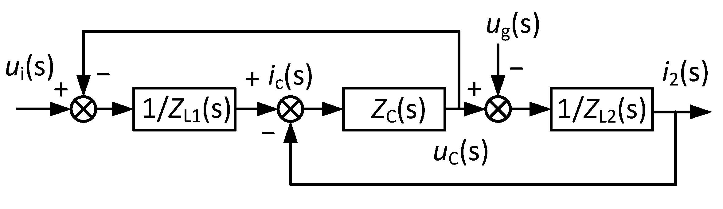
A block diagram of the single-phase FOLCL is shown in Figure 2.
In Figure 2, are the impedances of , , and , respectively. Their expressions are:
The transfer function from to can be derived as:
When , (9) can be written as:
3.2. Characteristics Analysis
3.2.1. Theoretical Analysis
Compared with L-type filters, conventional IOLCL filters can achieve better high-frequency harmonic attenuation capability. However, IOLCL filters have a resonant peak, which leads to system instability. Passive and active damping methods are used to suppress the resonant peak. For FOLCL filters, the resonance can be avoided by adjusting the component orders. From (9), the frequency domain expression of the FOLCL filter was written as:
To simplify the analysis, it was assumed that and was substituted into (11). With set when , (11) could be expressed as:
The magnitude–frequency and phase–frequency characteristics are expressed in (13) and (14), respectively:
When , , the denominator of , increases with the angular frequency, so decreases. In this case, there is no resonance in the magnitude–frequency characteristic. When , , . At this time, . When , . Thus, the magnitude–frequency characteristic has a resonant peak. Substituting back into (13), we had . The resonant frequency was determined only by the component values of , and , independently of and .
To sum up:
- When the resonant peak existed in the FOLCL filter, the resonant frequency was determined only by the values of and , independently of and . The resonant frequency was:
- When , the sufficient condition for the existence of resonance was . Compared with the IOLCL filter, the resonance could be effectively avoided by setting .
- When , and , there was a +180° phase jump at the resonance frequency. When , , and , there was a −180° phase jump at the resonance frequency.
The characteristics of the IOLCL and FOLCL filters are listed in Table 1.
3.2.2. Simulation Analysis
The inductor order was set to 0.8, 1.0, and 1.2, and the capacitor order was set to 0.8, 1.0, and 1.2 for each of these three cases. The corresponding bode plots are shown in Figure 3.
The capacitor order was set to 0.8, 1.0, and 1.2, and the inductor order was set to 0.8, 1.0, and 1.2 for each of these three cases. The bode plots are shown in Figure 4.
As shown from Figure 3 and Figure 4, when , , and (for example, the combination of and was (0.8, 1.2) or (1.0, 1.0)), the magnitude–frequency characteristic of the FOLCL filter had a resonant peak, and the phase–frequency characteristic had a −180° phase jump. When and (for example, the combination of and was (1.2, 0.8)), the magnitude–frequency characteristic of the FOLCL filter had a resonance peak, and the phase–frequency characteristic had a +180° phase jump. When (for example, the combination of and was (0.8, 0.8), (0.8, 1.0), (1.0, 0.8), (1.0, 1.2), (1.2, 1.0), or (1.2, 1.2)), the FOLCL filter showed no resonance peak. The resonant frequency measured from the figure was = 28,900 rad/s, which was basically equal to the theoretical value ( = 28,867.5 rad/s). It was also proved that the resonant frequency was independent of the inductor order and the capacitor order and was determined only by the values of , and .
Figure 3 also showed that when the inductor order was unchanged, and the capacitor order took different values, the frequency characteristics at low frequency bands were almost the same, but those at high frequency bands became different. This means that the capacitor order affected the frequency characteristics of the FOLCL filter only at high frequency bands. The inductor order determined the low-frequency characteristics of the FOLCL filter.
Similarly, Figure 4 showed that when the capacitor order was unchanged, and the inductor took different values, the slopes of the magnitude–frequency characteristic curves were different at all frequency bands. Furthermore, the phase–frequency characteristics were different from each other. This further shows that the frequency characteristic of the FOLCL filter at low frequency bands was determined by the inductor order , while the frequency characteristic at high frequency bands was determined by the orders and together.
4. Single-Phase Grid-Connected Inverter (GCI) based on the FOLCL Filter
4.1. System Structure
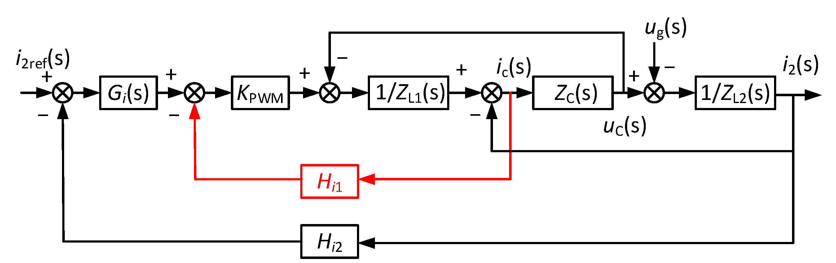
Figure 5 shows the single-phase FOGCI and its control system, where is the inverter-side inductor, is the filter capacitor, is the grid-side inductor, and these three taken together constitute a fractional-order LCL filter. For GCI, the primary goal is to control the grid current , synchronize it with the grid voltage , and make its RMS value track a given value . Since the dynamic of the voltage loop is much slower than that of the grid current loop, the grid current loop could be analyzed separately. and are the sampling coefficients of and , respectively. The sampled signal of is compared with its reference , and the error is fed into the current controller . The active damping of the resonance peak is achieved by capacitor current proportional feedback, and is the feedback coefficient. The capacitor current proportional feedback can be eliminated if , so the capacitor current feedback loop is shown in red in Figure 5, Figure 6 and Figure 8 to stress this problem. Subtracting the feedback signal from , the output of , yields the modulation wave .
4.2. FOGCI Based on Capacitor Current Proportional Feedback
According to Figure 5, the mathematical model of the LCL-type grid-connected inverter was obtained, as shown in Figure 6. is the transfer function of the modulation wave to the output voltage of the inverter bridge, where is the input voltage and is the magnitude of the triangular carrier. are the impedances of , , and , respectively, and their expressions are in (8). When , as in the IOGCI, the capacitor current proportional feedback had to be used to damp the resonance.
In order to derive its transfer function, the block diagram method was used to simplify the mathematical model, as shown in Figure 7.
According to (16), (17), and Figure 7, the open-loop transfer function of the IOGCI was derived as:
Similarly, the open-loop transfer function of the FOGCI was obtained as:
4.3. GCI without Capacitor Current Proportional Feedback
According to Figure 5, a control block diagram of a GCI without capacitor current proportional feedback when is shown in Figure 8. The capacitor current proportional feedback could be eliminated.
Figure 8.
Control block diagram of FOGCI without capacitor current proportional feedback (Capacitor current proportional feedback was eliminated).
Figure 8.
Control block diagram of FOGCI without capacitor current proportional feedback (Capacitor current proportional feedback was eliminated).

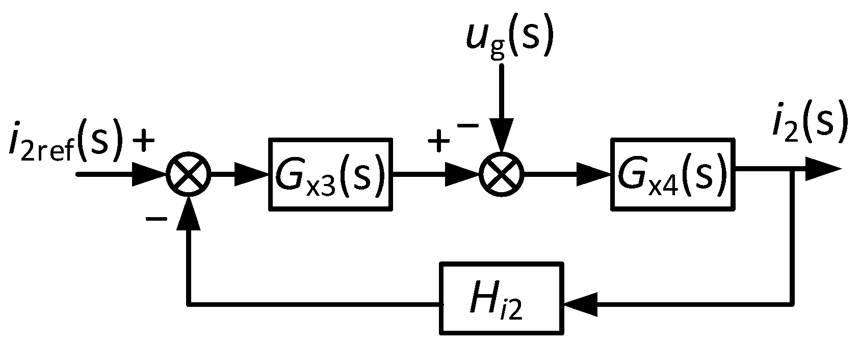
In order to derive the transfer function, the block diagram in Figure 8 was simplified as shown in Figure 9, where and are expressed in (20) and (21), respectively.
According to (20), (21), and Figure 9, the open-loop transfer function of the IOGCI was derived as:
Similarly, the open-loop transfer function of the FOGCI was expressed as:
4.4. Characteristic Analyses of the GCI System
In order to analyze the performance of the IOGCI and FOGCI, as well as the control effect of the IOPI and FOPI controllers, in detail, the open-loop transfer functions of the “IOGCI + IOPI”, “IOGCI + FOPI”, “FOGCI + IOPI”, and “FOGCI + FOPI” systems with capacitor current proportional feedback and the open-loop transfer functions of the “FOGCI + FOPI” and “FOGCI + IOPI” systems without capacitor current proportional feedback were derived as shown below.
The transfer functions of the IOPI and FOPI controllers are expressed in (24) and (25), respectively:
where are the proportional coefficient and integral coefficient, respectively, and λ is the integral order, 0 < λ < 2.
The open-loop transfer functions of the GCI systems based on proportional feedback of capacitor current were as follows. The loop gain of the “IOGCI + IOPI” system was deduced from (18) and (24) as:
The loop gain of the “IOGCI + FOPI” system was deduced from (18) and (25) as:
The loop gain of the “FOGCI + IOPI” system was deduced from (19) and (24) as:
The loop gain of the “FOGCI + FOPI” system was deduced from (19) and (25) as:
The open-loop transfer functions of the GCI systems without capacitor current proportional feedback were as follows. The loop gain of the “FOGCI + IOPI” system was deduced from (23) and (24) as:
The loop gain of the “FOGCI + FOPI” system was deduced from (23) and (25) as:
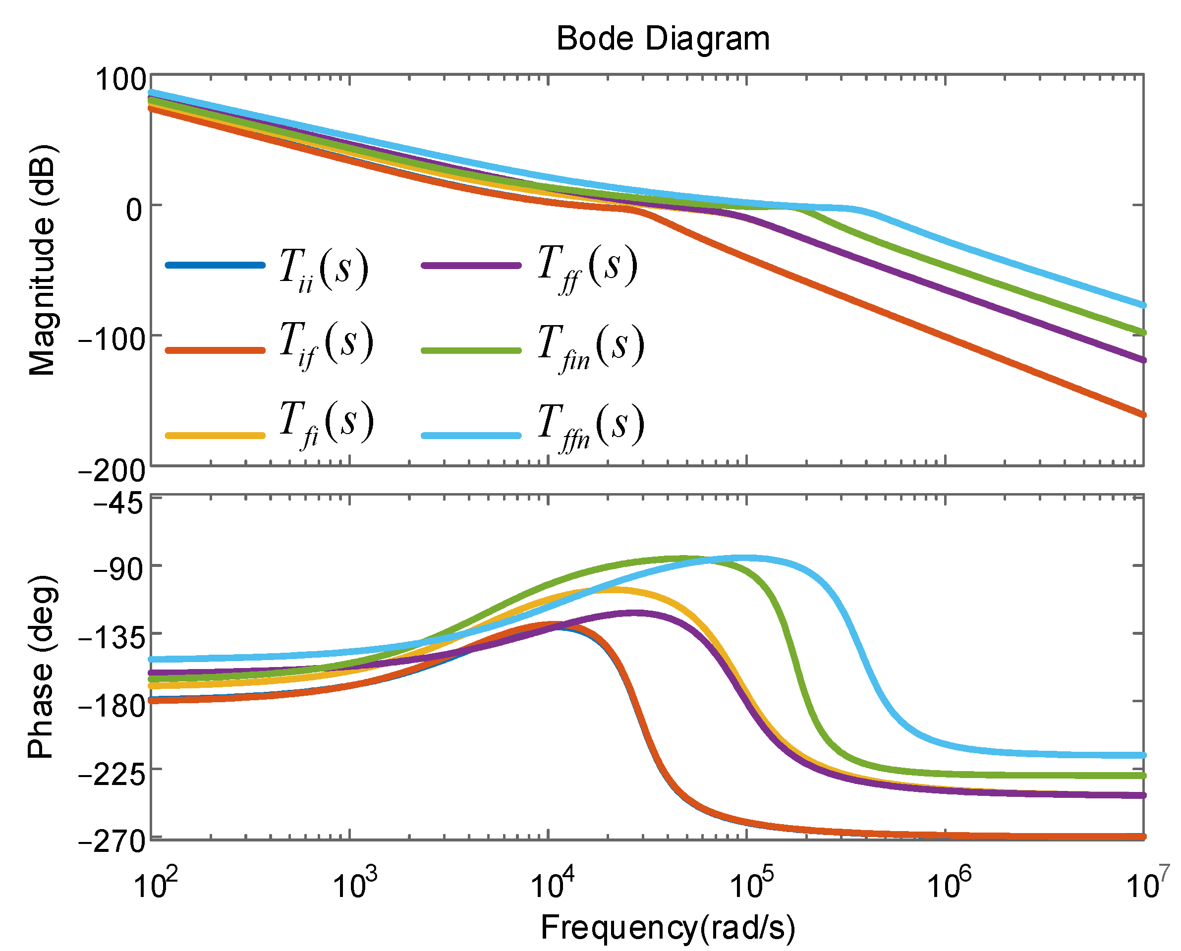
The bode plots of the loop gains in (26)–(31) are shown in Figure 10.
Table 2 shows the magnitude margins and phase margins of the bode plots in Figure 10. had larger magnitude and phase margins than . Under IOPI control and capacitor current proportional feedback, the FOGCI could be more stable and achieve faster dynamic response than the IOGCI. Moreover, had larger magnitude and phase margins than . This indicates that the FOGCI showed better performance than the IOGCI under FOPI control and capacitor current proportional feedback. had larger magnitude and phase margins than . However, had lower magnitude and phase margins than . Compared with IOPI control, FOPI control could improve the system performance of the IOGCI but could not improve that of the FOGCI when α + β = 2.
When α + β ≠ 2, the capacitor current proportional feedback could be removed. In this situation, had larger magnitude and phase margins than . Both FOPI control and IOPI control could obtain better performance for the FOGCI.
5. Simulation and Experimental Results
5.1. Fractional-Order Component Approximation
Since the fractional-order differential operator is an irrational function and thus cannot be directly implemented in numerical simulation, the improved Oustaloup filtering method was used to approximate the fractional-order differential operator by integer-order components. According to the fitted transfer function, fractance chain circuit models of the fractional-order inductor and capacitor were built. The operators and were approximated by fractance chain circuits; their bode plots are shown in Figure 11. The Oustaloup filtering method achieved good approximations at interesting frequency bands.
5.2. Simulation Results
In order to verify the correctness of the theoretical analysis, single-phase IOGCI and FOGCI simulation models with and without capacitor current proportional feedback were constructed, and IOPI and FOPI controllers are used to control each GCI, respectively. The main circuit parameters are shown in Table 3, and the controller parameters are shown in Table 4. The reference RMS value of the grid current was .
5.2.1. IOGCI and FOGCI with Capacitor Current Proportional Feedback
For the IOGCI, the orders of both the inductor and capacitor were equal to 1. The capacitor current feedback coefficient . First, the IOPI controller was used to regulate the grid current; the results are shown in Figure 12. The RMS value of was 27.30 A, and the THD was 4.14%. Then, the FOPI was employed to control the grid current and the integral order λ = 0.95; the simulation results are shown in Figure 13. The RMS value of was 27.30 A, and the THD was 1.93%.
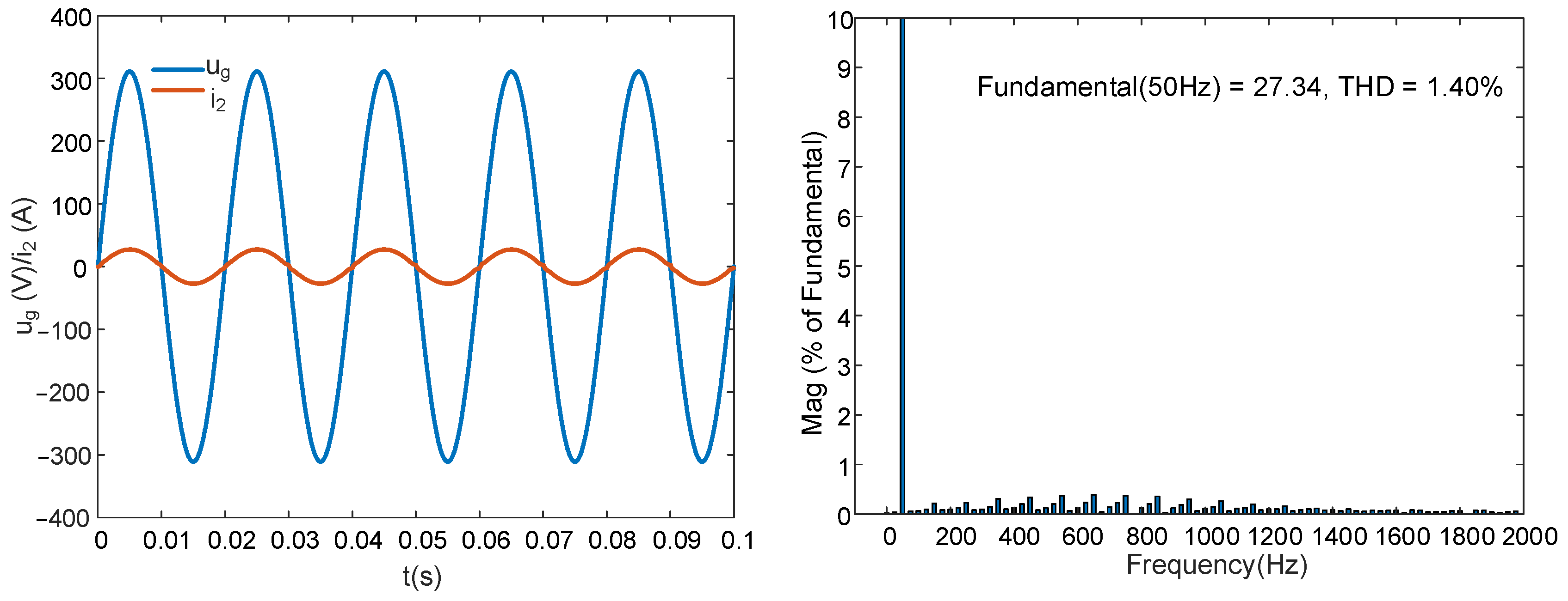
For the FOGCI, the inductor order and the capacitor order (). The capacitor current feedback coefficient . First, the IOPI controller was used to regulate the grid current; the results are shown in Figure 14. The system was stable, the RMS value of i2 was 27.34 A, and the THD was 1.40%. Then, the FOPI was employed to control the grid current, and the integral order λ = 0.9; the simulation results are shown in Figure 15. The system was stable, too, as the RMS value of i2 was 27.30 A and the THD was 0.94%.
The simulation results showed that each system had small stable-state error and that the grid current THD of the FOGCI was lower than that of the IOGCI under both IOPI and FOPI control.
5.2.2. FOGCI without Capacitor Current Proportional Feedback
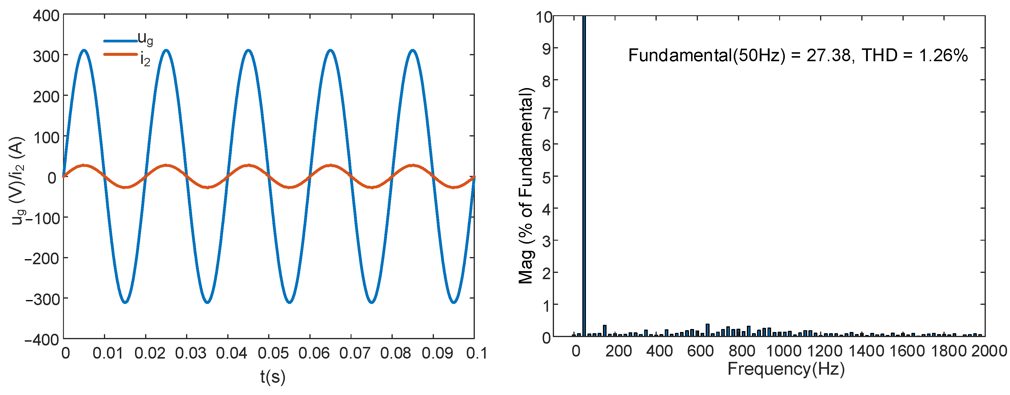
For the FOGCI, the capacitor current proportional feedback was omitted in this case. The inductor order , and the capacitor order (). First, the IOPI controller was used to regulate the grid current; the results are shown in Figure 16. The system was stable without active damping. The RMS value of was 27.38 A, and the THD was 1.26%. Then, the FOPI was employed to control the grid current, and the integral order λ = 0.9; the simulation results are shown in Figure 17. The RMS value of was 27.33 A, and the THD was 0.91%.
For the FOGCI, α + β = 2 (α = 1.2, β = 0.8), and the IOPI controller was used to regulate the grid current at the beginning. The capacitor current feedback coefficient . When t = 0.05 s, was set to 0, and the system became unstable, as shown in Figure 18.
The simulation results showed that under FOPI control, the FOGCI without capacitor current proportional feedback had lower THD than it did under IOPI control. Compared with the results of the GCI with capacitor current proportional feedback, the FOGCI without capacitor current proportional feedback had slightly increased stable-state error but a smaller grid current THD.
Some conclusions were drawn according to the simulation results:
- With or without capacitor current proportional feedback, the FOGCI showed better system performance than the IOGCI.
- For GCI systems, the overall control effect of the FOPI controller was better than that of the IOPI controller.
- Compared with the FOGCI based on capacitor current proportional feedback when , the FOGCI without capacitor current proportional feedback when obtained lower grid current THD and simplified the control system.
- When , the FOGCI without capacitor current proportional feedback could not guarantee system stability.
5.3. Experimental Results
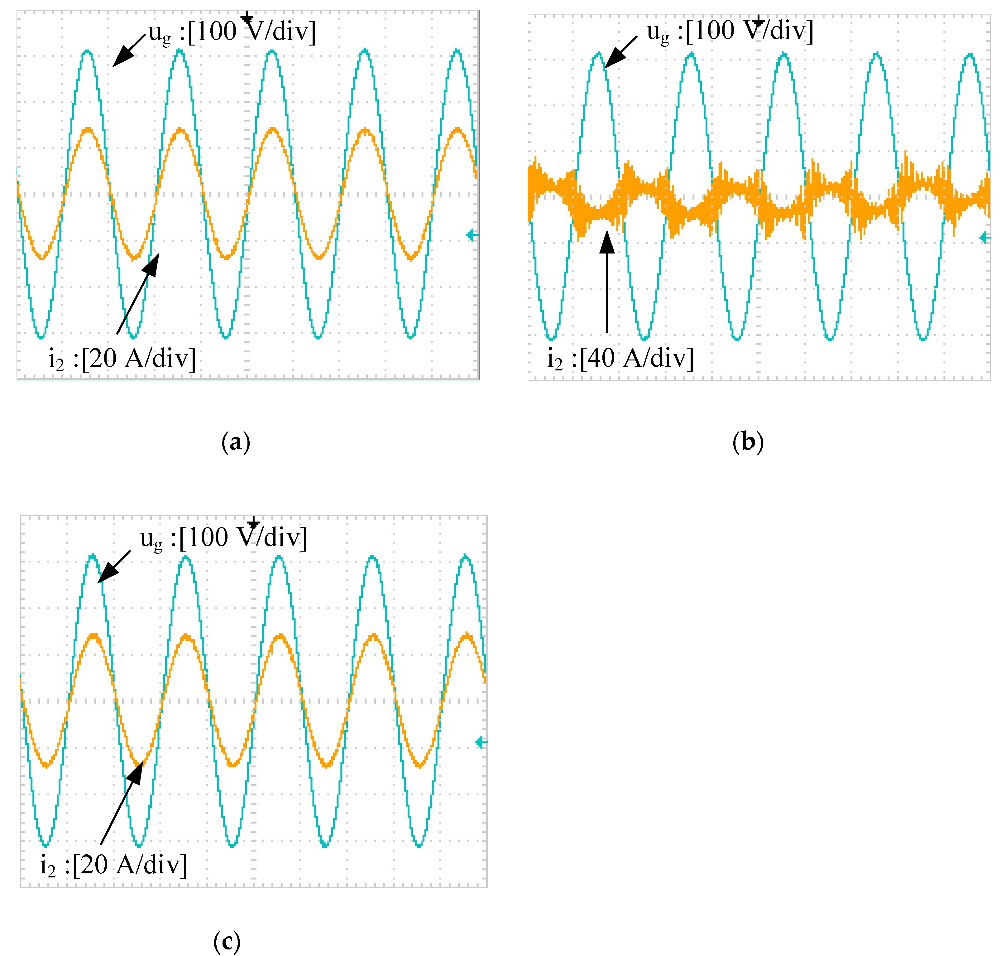
A hardware-in-the-loop experimental instrument was used to test the circuit. The experimental system consisted of a NI PXIe-1082 chassis, a computer, and an oscilloscope. The computer downloaded a Simulink model to the chassis through the StarSim HIL software (Version 4.6, Shanghai, China). Three cases were studied: (1) Case I: FOGCI with capacitor current proportional feedback, where the inductor order and capacitor order satisfy (); (2) Case II: FOGCI without capacitor current proportional feedback, where (); (3) Case III: FOGCI without capacitor current proportional feedback, where (). The results are shown in Figure 19. The system was stable in cases I and III but unstable in case II.
6. Conclusions
In this paper, the modeling and control problems of a grid-connected inverter based on an FOLCL filter were studied. A mathematical model of the FOLCL filter was derived, and its characteristics were analyzed. Then, the necessary and sufficient conditions of resonance was determined. Based on this, by rationally selecting the inductor and capacitor orders, the resonance of the FOLCL filter could be effectively avoided, which could allow eliminating the damper in the control system. Moreover, through the analysis of six types of GCI systems, it was found that compared with the “IOGCI + IOPI” system, the “FOGCI + FOPI” system without capacitor current proportional feedback was simpler and had greater magnitude and phase margins. In addition, the FOGCI had lower grid current THD than the IOGCI. Simulation and hardware-in-the-loop experiments were conducted, and the results were consistent with the theoretical analyses.
Author Contributions
Conceptualization, X.W. and J.C.; methodology, X.W.; investigation, J.C. and X.W.; writing—original draft preparation, J.C.; writing—review and editing, X.W.; supervision, X.W. All authors have read and agreed to the published version of the manuscript.
Funding
This work was supported by the Guangzhou Science and Technology Plan Project, no. 202102010404.
Institutional Review Board Statement
Not applicable.
Informed Consent Statement
Not applicable.
Conflicts of Interest
The authors declare no conflict of interest.
References
- Blaabjerg, F.; Teodorescu, R.; Liserre, M.; Timbus, A.V. Overview of control and grid synchronization for distributed power generation systems. IEEE Trans. Ind. Electron. 2006, 53, 1398–1409. [Google Scholar] [CrossRef] [Green Version]
- Prodanovic, M.; Green, T.C. High-quality power generation through distributed control of a power park microgrid. IEEE Trans. Ind. Electron. 2006, 53, 1471–1482. [Google Scholar] [CrossRef] [Green Version]
- IEEE Standard Committee. IEEE Standard for Interconnection and Interoperability of Distributed Energy Resources with Associated Electric Power Systems Interfaces: 1547-2003; IEEE: Piscataway, NJ, USA, 2003. [Google Scholar]
- IEEE Standard Committee. IEEE Recommended Practices and Requirements for Harmonic Control in Electric Power System: 519-1992; IEEE: Piscataway, NJ, USA, 2004. [Google Scholar]
- Twining, E.; Holmes, D.G. Grid current regulation of a three-phase voltage source inverter with an LCL input filter. IEEE Trans. Power Electron. 2003, 18, 888–895. [Google Scholar] [CrossRef] [Green Version]
- Liserre, M.; Dell’Aquila, A.; Blaabjerg, F. Genetic algorithm-based design of the active damping for an LCL-filter three-phase active rectifier. IEEE Trans. Power Electron. 2004, 19, 76–86. [Google Scholar] [CrossRef]
- Liserre, M.; Blaabjerg, F.; Hansen, S. Design and control of an LCL-filter-based three-phase active rectifier. IEEE Trans. Ind. Appl. 2005, 41, 1281–1291. [Google Scholar] [CrossRef]
- Muhlethaler, J.; Schweizer, M.; Blattmann, R.; Kolar, J.W.; Ecklebe, A. Optimal Design of LCL Harmonic Filters for Three-Phase PFC Rectifiers. IEEE Trans. Power Electron. 2013, 28, 3114–3125. [Google Scholar] [CrossRef]
- Wu, W.M.; He, Y.B.; Tang, T.H.; Blaabjerg, F. A New Design Method for the Passive Damped LCL and LLCL Filter-Based Single-Phase Grid-Tied Inverter. IEEE Trans. Ind. Electron. 2013, 60, 4339–4350. [Google Scholar] [CrossRef]
- Liserre, M.; Teodorescu, R.; Blaabjerg, F. Stability of photovoltaic and wind turbine grid-connected inverters for a large set of grid impedance values. IEEE Trans. Power Electron. 2006, 21, 263–272. [Google Scholar] [CrossRef]
- Liserre, M.; Dell’Aquila, A.; Blaabjerg, F. Stability improvements of an LCL-filter based three-phase active rectifier. In Proceedings of the 33rd IEEE Annual Power Electronics Specialists Conference (PESC02), Carins, Australia, 23–27 June 2002; pp. 1195–1201. [Google Scholar]
- Bahrani, B.; Vasiladiotis, M.; Rufer, A. High-order vector control of grid-connected voltage-source converters with LCL-filters. IEEE Trans. Ind. Electron. 2014, 61, 2767–2775. [Google Scholar] [CrossRef]
- Wehmuth, G.R.; Busarello, T.D.C.; Peres, A. Step-by-step design procedure for LCL-type single-phase grid connected inverter using digital proportional-resonant controller with capacitor-current feedback. In Proceedings of the 13th Annual IEEE Green Technologies Conference (GreenTech), Denver, CO, 7–9 April 2021; pp. 448–454. [Google Scholar]
- Shen, G.Q.; Xu, D.H.; Cao, L.P.; Zhu, X.C. An improved control strategy for grid-connected voltage source inverters with an LCL filter. IEEE Trans. Power Electron. 2008, 23, 1899–1906. [Google Scholar] [CrossRef]
- He, J.W.; Li, Y.W. Generalized closed-loop control (GCC) schemes with embedded virtual imepdances for voltage source converters. In Proceedings of the IEEE Energy Conversion Congress and Exposition (ECCE), Phoenix, AZ, USA, 17–22 September 2011; pp. 479–486. [Google Scholar]
- Wang, T.C.Y.; Ye, Z.H.; Sinha, G.; Yuan, X.M. Output filter design for a grid-interconnected three-phase inverter. In Proceedings of the 34th Annual IEEE Power Electronics Specialists Conference, Acapulco, Mexico, 15–19 June 2003; pp. 779–784. [Google Scholar]
- Dannehl, J.; Liserre, M.; Fuchs, F.W. Filter-based active damping of voltage source converters with LCL filter. IEEE Trans. Ind. Electron. 2011, 58, 3623–3633. [Google Scholar] [CrossRef]
- Blasko, V.; Kaura, V. A novel control to actively damp resonance in input LC filter of a three phase voltage source converter. In Proceedings of the 11th Annual Applied Power Electronics Conference and Exposition (APEC 96), San Jose, CA, USA, 3–7 March 1996; pp. 545–551. [Google Scholar]
- Maamir, F.; Guiatni, M.; El Hachemi, H.; Ali, D. Auto-tuning of fractional-order PI controller using particle swarm optimization for thermal device. In Proceedings of the 2015 4th International Conference on Electrical Engineering (ICEE), Boumerdes, Algeria, 13–15 December 2015; pp. 174–179. [Google Scholar]
- De Keyser, R.; Muresan, C.I.; Ionescu, C.M. A novel auto-tuning method for fractional order PI/PD controllers. ISA Trans. 2016, 62, 268–275. [Google Scholar] [CrossRef] [PubMed]
- Erenturk, K. Fractional-order PIλDμ and active disturbance rejection control of nonlinear two-mass drive system. IEEE Trans. Ind. Electron. 2013, 60, 3806–3813. [Google Scholar] [CrossRef]
- Xu, J.H.; Li, X.C.; Meng, X.R.; Qin, J.B.; Liu, H. Modeling and analysis of a single-phase fractional-order voltage source pulse width modulation rectifier. J. Power Sources 2020, 479, 12. [Google Scholar] [CrossRef]
- Freeborn, T.J.; Maundy, B.; Elwakil, A.S. Measurement of supercapacitor fractional-order model parameters from voltage-excited step response. IEEE Jour. Emer. Select. Top. Circu. Syste. 2013, 3, 367–376. [Google Scholar] [CrossRef]
- Chen, X.; Xi, L.; Zhang, Y.N.; Ma, H.; Huang, Y.H.; Chen, Y.Q. Fractional techniques to characterize non-solid aluminum electrolytic capacitor for power electronic applications. Nonlinear Dyn. 2019, 98, 3125–3141. [Google Scholar] [CrossRef]
- Allagui, A.; Freeborn, T.J.; Elwakil, A.S.; Fouda, M.E.; Maundy, B.J.; Radwan, A.G.; Said, Z.; Abdelkareem, M.A. Review of fractional-order electrical characterization of supercapacitor. J. Power Sources 2018, 400, 457–467. [Google Scholar] [CrossRef]
- Machado, J.A.T.; Galhano, A. Fractional order inductive phenomena based on the skin effect. Nonlinear Dyn. 2012, 68, 107–115. [Google Scholar] [CrossRef]
- Jesus, I.S.; Machado, J.A.T. Development of fractional order capacitor based on electrolyte processes. Nonlinear Dyn. 2009, 56, 45–55. [Google Scholar] [CrossRef] [Green Version]
- Kartci, A.; Agambayev, A.; Herencsar, N.; Salama, K.N. Series-, parallel-, and inter-connection of solid-state arbitrary fractional-order capacitor: Theoretical study and experimental verification. IEEE Access 2018, 6, 10933–10943. [Google Scholar] [CrossRef]
- Bertsias, P.; Psychalinos, C.; Radwan, A.G.; Elwakil, A.S. High-frequency capacitorless fractional-order CPE and FI emulator. Circuits Syst. Signal Process. 2018, 37, 2694–2713. [Google Scholar] [CrossRef]
- Sarafraz, M.S.; Tavazoei, M.S. Passive realization of fractional-order impedances by a fractional element and RLC components: Conditions and procedure. IEEE Trans. Circuits Syst. I-Regul. Pap. 2017, 64, 585–595. [Google Scholar] [CrossRef]
- Radwan, A.G.; Soliman, A.M.; Elwakil, A.S. Design equations for fractional-order sinusoidal oscillators: Four practical circuit examples. Int. J. Circuit Theory Appl. 2008, 36, 473–492. [Google Scholar] [CrossRef]
- Semary, M.S.; Fouda, M.E.; Hassan, H.N.; Radwan, A.G. Realization of fractional-order capacitor based on passive symmetric network. J. Adv. Res. 2019, 18, 147–159. [Google Scholar] [CrossRef] [PubMed]
- Chen, X.; Chen, Y.F.; Zhang, B.; Qiu, D.Y. A Modeling and analysis method for fractional-order DC-DC converters. IEEE Trans. Power Electron. 2017, 32, 7034–7044. [Google Scholar] [CrossRef]
- Wu, C.J.; Si, G.Q.; Zhang, Y.B.; Yang, N.N. The fractional-order state-space averaging modeling of the Buck Boost DC/DC converter in discontinuous conduction mode and the performance analysis. Nonlinear Dyn. 2015, 79, 689–703. [Google Scholar] [CrossRef]
- Tan, C.; Liang, Z.S. Modeling and simulation analysis of fractional-order Boost converter in pseudo-continuous conduction mode. Acta Phys. Sin. 2014, 63, 10. [Google Scholar] [CrossRef]
- Ahmad, W. Power factor correction using fractional capacitors. In Proceedings of the IEEE International Symposium on Circuits and Systems, Bangkok, Thailand, 25–28 May 2003; pp. 5–7. [Google Scholar]
- Sharma, M.; Rajpurohit, B.S.; Agnihotri, S.; Rathore, A.K. Development of fractional order modeling of voltage source converters. IEEE Access 2020, 8, 131750–131759. [Google Scholar] [CrossRef]
- Xu, J.H.; Li, X.C.; Liu, H.; Meng, X.R. Fractional-order modeling and analysis of a three-phase voltage source PWM rectifier. IEEE Access 2020, 8, 13507–13515. [Google Scholar] [CrossRef]
- El-Khazali, R. Fractional-order LCαL filter-based grid connected PV systems. In Proceedings of the 62nd IEEE International Midwest Symposium on Circuits and Systems (MWSCAS), Dallas, TX, USA, 4–7 August 2019; pp. 533–536. [Google Scholar]
- Podlubny, I. Fractional-order systems and PIλDμ-controllers. IEEE Trans. Autom. Control 1999, 44, 208–214. [Google Scholar] [CrossRef]
- Martinez, R.; Bolea, Y.; Grau, A.; Martinez, H. LPV model for PV cells and fractional control of DC/DC converter for photovoltaic systems. In Proceedings of the 20th IEEE International Symposium on Industrial Electronics (ISIE), Gdansk, Poland, 27–30 June 2011. [Google Scholar]
- Jiang, P.; Lv, H.J.; Wang, L.Y. Study on Control of Single Phase Grid-Connected Inverter Based on Fractional Order PI Controller. In Proceedings of the 2nd International Conference on Materials Science, Machinery and Energy Engineering (MSMEE), Dalian, China, 13–14 May 2017; pp. 1414–1420. [Google Scholar]
- Ghoudelbourk, S.; Azar, A.T.; Dib, D. Three-level (NPC) shunt active power filter based on fuzzy logic and fractional-order PI controller. Int. J. Autom. Control 2021, 15, 149–169. [Google Scholar] [CrossRef]
- Podlubny. Fractional Differential Equations.; USA Academic: New York, NY, USA, 1999. [Google Scholar]
- Monje, C.A.; Chen, Y.; Vinagre, B.M.; Xue, D. Fractional Order Systems and Controls: Fundamentals and Applications; Springer: London, UK, 2010. [Google Scholar]
- Petras. Fractional calculus. In Fractional-Order Nonlinear Systems; Higher Education: Beijing, China, 2011. [Google Scholar]
- Ruan, X.; Wang, X.; Pan, D. Control Techniques for LCL-Type Grid-Connected Inverters; Springer: Singapore, 2017. [Google Scholar]
Figure 1.
Topology of a fractional-order LCL filter.

Figure 2.
Block diagram of single-phase FOLCL filter.

Figure 3.
Bode plots of FOLCL filter as α changed: (a) ; (b) ; (c) .


Figure 4.
Bode plots of FOLCL filter as β changed: (a) ; (b) ; (c) .


Figure 5.
System structure of the single-phase FOGCI (Capacitor current proportional feedback can be eliminated if α + β ≠ 2).
Figure 5.
System structure of the single-phase FOGCI (Capacitor current proportional feedback can be eliminated if α + β ≠ 2).

Figure 6.
Block diagram of the FOGCI control system with capacitor current proportional feedback (Capacitor current proportional feedback can be eliminated if α + β ≠ 2).
Figure 6.
Block diagram of the FOGCI control system with capacitor current proportional feedback (Capacitor current proportional feedback can be eliminated if α + β ≠ 2).

Figure 7.
Simplified block diagram of the GCI control system with capacitor current proportional feedback.
Figure 7.
Simplified block diagram of the GCI control system with capacitor current proportional feedback.

Figure 9.
Simplified diagram of the GCI without capacitor current proportional feedback.

Figure 10.
Bode plots of the loop gains of the GCIs.

Figure 11.
Bode plots of approximated fractance chain circuits: (a) ; (b) .

Figure 12.
Simulation results of the “IOGCI + IOPI” system.

Figure 13.
Simulation results of the “IOGCI + FOPI” system.

Figure 14.
Simulation results of the “FOGCI + IOPI” system with α + β = 2.

Figure 15.
Simulation results of the “FOGCI + FOPI” system with α + β = 2.

Figure 16.
Simulation results of the “FOGCI + IOPI” system with α + β ≠ 2.

Figure 17.
Simulation results of the “FOGCI + FOPI” system with α + β ≠ 2.

Figure 18.
Simulation results of the “FOGCI + IOPI” system with α + β ≠ 2 (α = 1.2, β = 0.8).

Figure 19.
Experimental results: (a) FOGCI with capacitor current proportional feedback, where (α = 1.2, β = 0.8); (b) FOGCI without capacitor current proportional feedback, where (α = 1.2, β = 0.8); (c) FOGCI without capacitor current proportional feedback, where (α = 0.8, β = 0.8).
Figure 19.
Experimental results: (a) FOGCI with capacitor current proportional feedback, where (α = 1.2, β = 0.8); (b) FOGCI without capacitor current proportional feedback, where (α = 1.2, β = 0.8); (c) FOGCI without capacitor current proportional feedback, where (α = 0.8, β = 0.8).


Table 1.
Characteristics comparison of IOLCL and FOLCL filters.
| Characteristics | IOLCL Filter | FOLCL Filter | Statement |
| Number of variables | ) | ) | is the order of the inductor and is the order of the capacitor |
| Transfer function | |||
| Resonance peak | exists | is a sufficient condition for the existence of a resonance peak in the FOLCL filter | |
Table 2.
Magnitude and phase margins of the loop gains.
| Loop Gain | Magnitude Margin | Phase Margin |
| 4.29 dB | 48.0° | |
| 4.42 dB | 49.9° | |
| 11.4 dB | 71.1° | |
| 9.91 dB | 56.7° | |
| 5.03 dB | 93.2° | |
| 10.1 dB | 93.7° |
Table 3.
Single-phase GCI parameters [47].
Table 3.
Single-phase GCI parameters [47].
| Parameters | Symbols | Numerical Value | Parameters | Symbols | Numerical Value |
| DC input voltage | 360 V | Filter capacitor | 10 μF | ||
| RMS value of grid voltage | 220 V | Grid-side inductor | 150 μH | ||
| Rated power of inverter | 6 kW | Carrier magnitude | 3.05 V | ||
| Grid frequency | 50 Hz | Capacitor current sampling coefficient | 0.1 or 0 | ||
| Switching frequency | 10 kHz | Grid current sampling coefficient | 0.15 | ||
| Inverter-side inductor | 600 μH |
Table 4.
Controller parameters.
| GCI Model | Controller | Kp | Ki | λ |
| FOGCI (α + β = 2, capacitor current proportional feedback was used) | IOPI | 0.443 | 2250 | 1 |
| FOPI | 0.442 | 2248 | 0.90 | |
| IOGCI (capacitor current proportional feedback was used) | IOPI | 0.450 | 2200 | 1 |
| FOPI | 0.450 | 2582 | 1.01 | |
| FOGCI (α + β ≠ 2, capacitor current proportional feedback was not used) | IOPI FOPI | 0.630 0.550 | 2500 2400 | 1 0.90 |
Publisher’s Note: MDPI stays neutral with regard to jurisdictional claims in published maps and institutional affiliations. |
© 2022 by the authors. Licensee MDPI, Basel, Switzerland. This article is an open access article distributed under the terms and conditions of the Creative Commons Attribution (CC BY) license (https://creativecommons.org/licenses/by/4.0/).
Share and Cite
MDPI and ACS Style
Wang, X.; Cai, J. Grid-Connected Inverter Based on a Resonance-Free Fractional-Order LCL Filter. Fractal Fract. 2022, 6, 374. https://0-doi-org.brum.beds.ac.uk/10.3390/fractalfract6070374
AMA Style
Wang X, Cai J. Grid-Connected Inverter Based on a Resonance-Free Fractional-Order LCL Filter. Fractal and Fractional. 2022; 6(7):374. https://0-doi-org.brum.beds.ac.uk/10.3390/fractalfract6070374
Chicago/Turabian StyleWang, Xiaogang, and Junhui Cai. 2022. "Grid-Connected Inverter Based on a Resonance-Free Fractional-Order LCL Filter" Fractal and Fractional 6, no. 7: 374. https://0-doi-org.brum.beds.ac.uk/10.3390/fractalfract6070374