1. Introduction
Autonomous underwater vehicles (AUVs) are a crucial technical platform for ocean information acquisition and autonomous operation. They have extensive application prospects, such as marine environment observation, marine resources exploration and security defense. Nevertheless, motion control systems for AUV have become very challenging due to their high nonlinearity, strong coupling, model parameter uncertainties and external disturbances. In addition, an AUV system is usually designed to be underactuated to save cost and improve propulsion efficiency.
With regard to the motion control of underactuated AUV, a variety of control algorithms are available, including proportional-integral-derivative (PID) control, backstepping control, fuzzy logic control, and sliding mode control [
1,
2,
3,
4,
5,
6,
7]. In [
4], a single-input fuzzy logic controller (SIFLC) was proposed for AUV depth control. Simulation results show that the SIFLC gives an identical response as Mamdani and T-S type FLC to the same input sets, while its execution time is more than two orders of magnitude faster than the conventional FLC. In [
6], a switching control algorithm based on active disturbance rejection control (ADRC) and fuzzy logic control was applied to the depth control of a self-developed AUV. Numerical simulations showed that the proposed method is more efficient in suppressing external disturbances and inner signal transmission disturbance than PID controller.
Fractional calculus is an extension of traditional integral calculus, it describes the fractal dimension of space. In recent years, its applications in the control field, such as fractional-order model [
8,
9], fractional-order control algorithm [
10,
11,
12], fractional-order optimization algorithm [
13,
14], have attracted significant research attention. Furthermore, stability analysis for fractional-order control systems have been proposed in several studies [
15,
16,
17]. A fractional-order, proportional–integral–derivative (FOPID) controller has been proposed by Podlubny. Their proposed controller has two additional parameters: integral order and differential order compared with a PID controller [
18]. In [
19], an optimized FOPID controller for improved transient control performance was applied to an AUV yaw control system. In addition, a fractional-order Mamdani fuzzy logic controller has been proposed for vehicle nonlinear active suspension, which effectively improves ride comfort and handling stability [
20]. However, there has been no report on the application of fractional-order fuzzy logic control in AUV motion.
In this paper, a single-input fractional-order fuzzy logic controller (SIFOFLC) is proposed and applied to an AUV motion control system. Its control input was simplified to a single variable known as distance variable by applying the signed distance method [
21], which aims to reduce the computation burden and complex parameter tuning process. Furthermore, a fractional calculus operator was applied to the enhanced FLC due to its recognized ability to increase the controller’s flexibility and adaptability. With respect to the controller parameters, we developed and applied a hybrid particle swarm optimization (HPSO) algorithm to obtain optimal control performance. Unlike a conventional PSO algorithm, this includes the local optimal particle term to avoid falling into local optimal region, and the fitness value function includes both steady-state performance and transient performance of an AUV motion control system. To verify the effectiveness of SIFOFLC, we conducted comparative numerical simulations of spiral dive motion control. The object of study, REMUS-100 AUV, was developed by Woods Hole Oceanographic Institution [
22], while the simulation was performed using the marine systems simulator (MSS) by Fossen and Perez [
23]. Simulation results show that, compared with a FOPID controller and conventional T-S FLC, the SIFOFLC is more efficient in reducing angular velocity oscillations, shortening settling time and improving control accuracy.
The remainder of this paper is organized as follows.
Section 2 discusses the six degrees of freedom nonlinear motion equations of AUV. The SIFOFLC design is introduced in
Section 3, along with its advantages compared with traditional T-S FLC. In
Section 4, the HPSO algorithm is described and is applied to various control systems to obtain optimal parameters. To verify the effectiveness of the proposed method, simulations and numerical comparisons are carried out in
Section 5. Finally, some concluding remarks are presented in
Section 6.
2. Kinematic and Dynamic Modeling of AUV
Six degrees of freedom motion equations of AUV can be described using the earth-fixed coordinate system and body-fixed coordinate system shown in
Figure 1, both of which are right-handed. The earth-fixed coordinate system
has its origin
fixed to the earth, and the body-fixed coordinate system
is a moving reference frame with its origin
fixed to AUV center of buoyancy.
The general motion of a vehicle in six degrees of freedom can be described with the following vectors:
where
describes the position and orientation of the vehicle with respect to the earth-fixed reference frame,
denotes the linear and angular velocities with respect to the body-fixed reference frame, and
describes the total forces and moments acting on the vehicle in the body-fixed reference frame.
The coordinate transformation of the translational velocity between earth-fixed and body-fixed coordinate systems can be expressed as
where
The coordinate transformation relates rotational velocity between two coordinate systems and can be described as
where
The locations of the AUV centers of gravity and buoyancy are defined in the body-fixed coordinate system as follows:
Based on the theory of rigid body dynamics and the analysis of total forces and moments acting on AUV, the nonlinear motion equations for the REMUS vehicle in six degrees of freedom can be expressed as follows [
24]:
where
is AUV’s mass,
are the moments of inertia of AUV to three coordinate axes,
are hydrostatics,
are hydrodynamic drag coefficients,
are lift coefficients and lift moment coefficients of body and control fins, respectively,
are propeller thrust and torque, respectively, and
are rudder angle and stern plane angle, respectively. The remaining coefficients are added mass coefficients.
Separate the acceleration terms from the other terms in the equations of AUV motion so that the equations can be summarized in matrix form as follows:
where
refer to the sum of terms without acceleration. So far, six degrees of freedom nonlinear motion equations of AUV can be obtained by combining (4) with (1) and (2).
3. Design of SIFOFLC
3.1. Fundamentals of Fractional Calculus
Fractional calculus, essentially the non-integer order calculus, has the same history as integer order calculus. The three frequently used definitions of fractional calculus are the Grunwald–Letnikov definition, the Riemann–Liouville definition and the Caputo definition [
25].
We consider the Caputo definition in this study because of its wide applications in engineering problems, the fractional integral and derivative by Caputo definition are as follows:
where
represents the fractional calculus operator,
is a continuous function and
denotes the initial time.
represents the fractional-order,
.
denotes the Gamma function as in (7).
In the numerical simulations, we adopt the standard Oustaloup approximation method to obtain the consistent frequency characteristics as fractional differential operator. A rational transfer function in the form of zero-pole type is described according to the Oustaloup method, that is the order of filter, is the selected frequency bound. The zero and pole are defined as and , which divide the frequency band into 2N + 1 intervals.
The Oustaloup rational approximation is described as
where
,
,
,
.
3.2. Structure Design of SIFOFLC
A fuzzy logic controller has four components: knowledge base, inference engine, fuzzification interface, and defuzzification interface [
26]. The basic structure of a two-dimensional fuzzy logic controller is described as in
Figure 2, where the continuous input signal,
and
, convert to the membership degree vector of the fuzzy variables through a fuzzification interface, the inference engine carries out rule inference and actual output signal is obtained through defuzzification interface. The data base denotes membership functions of the total input and output variables and the rule base is performed using a collection of fuzzy if–then rules by expert experience, both of which make up the knowledge base.
Compared with the linear controller, fuzzy logic control method is more robust and suitable for complex control requirements, while its complex decision-making process brings a challenge for real-time operation. Thus, we aim to adjust the controller structure to reduce computation burden and achieve better performance.
Typically, a fuzzy logic controller has two control inputs, namely error
and its derivative
. It is common for its rule table to have the same output membership in a diagonal direction, something known as the Toeplitz structure, as shown in
Table 1 [
4]. In addition, each position on a diagonal line has the same distance from the main diagonal line of rule table. Thus, instead of using two-variable input sets
, the corresponding control output can be obtained using the distance between input signal and the main diagonal line. This finding was first proposed by Choi et al. and is known as the signed distance method [
21]. To derive the distance,
, a two-dimensional space of
and
is established as shown in
Figure 3.
The main diagonal line of the rule table is presented as a straight line crossing over the origin, whose function is . In this case, the distance from point to can be obtained as .
Furthermore, in order to achieve better control performance, we extend the derivative of error signal to fractional order, thus the distance variable is described as
where
is the fractional order of error signal and it further increases degrees of freedom and complexity of the controller.
Based on the above analysis, the overall structure of SIFLC can be depicted as in
Figure 4. The distance variable is obtained through linear combination of error signal and its fractional derivative, the inner fuzzy logic controller is single input single output (SISO) and the final output
is obtained by multiplying
with the scale factor, which is denoted as
. We set
to 1. Thus, in addition to the membership functions, there are two adjustable parameters in the SIFOFLC, namely
and
.
3.3. Characteristics of SIFOFLC
In this section, the SIFOFLC and T-S FLC used in the simulation research of
Section 4 are proposed and the superiority of SIFOFLC is presented through comparison.
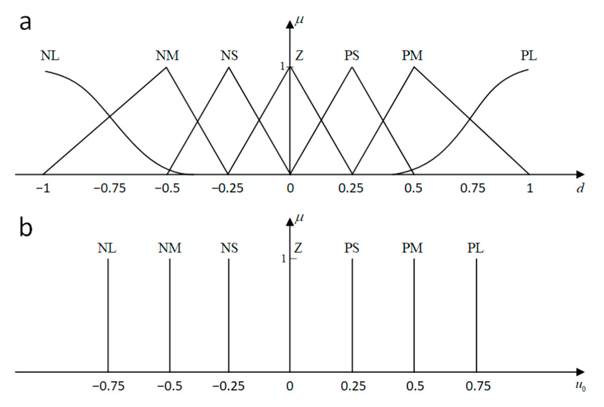
To the SIFOFLC, the fuzzy sets of
and
are both {NL, NM, NS, Z, PS, PM, PL} and the membership functions are shown in
Figure 5. The membership functions of
include both S shape and triangular shape membership functions, with a singleton value membership function for
. In this case, the rule table is reduced to the one-dimensional vector as shown in
Table 2.
Based on the work mentioned above, the proposed SIFOFLC has the following advantages compared to conventional FLC:
- (1)
Simplified design process.
For the two-dimensional FLC, the membership functions for error input and its derivative are required simultaneously, which means a lengthy complex tuning process. With the only input, , the parameter tuning process for SIFOFLC is significantly reduced. Further, in a two-dimensional FLC, the number of fuzzy rules to be inferred is the square of n, which is the size of the fuzzy set. The distinguishing feature of SIFLC is that it requires only n rules, which is an exponential decay. Typically, better performance can be obtained with more a complicated control algorithm, such as the increase of fuzzy sets and rules, which further reveals the superiority of SIFOFLC.
- (2)
Reduced computation burden.
The control surfaces for the SIFOFLC and conventional T-S FLC are respectively shown in
Figure 6 and
Figure 7. Compared with the complex curved surface of T-S FLC, the control surface of SIFOFLC has been simplified to a linear with different slopes. Thus, the computation burden of controller operation, which includes fuzzification, fuzzy inference and defuzzification, has been significantly reduced.
4. Parameter Optimization for Three Controllers with HPSO Algorithm
In this section, the HPSO algorithm is developed and applied to optimize the controller parameters. Except for the SIFOFLC, the T-S FLC and FOPID control systems are optimized for further comparison in
Section 5, as the SIFOFLC algorithm essentially originates from the T-S FLC, and because the FOPID controller is the most extensively used fractional order control algorithm.
It is necessary to mention that our optimization and research scenario is the spiral dive motion control of REMUS-100 AUV. It is performed using Marine Systems Simulator (MSS), which is a MATLAB toolbox and offers a set of tools for marine engineering researchers [
23]. Some research details are as follows: The target depth of AUV motion linearly increases from 0 m to 30 m and the target yaw angle from
to
. The simulation time is 300 s and the input constraint of fins is set to
in accordance with [
24]. Furthermore, the external disturbances are ignored.
Figure 8 illustrates the block diagram of an AUV motion control system. The propeller speed is fixed at 1500 r/m so that the cruise speed maintains a constant value. In this case, the target trajectory is obtained with heading controller and depth controller.
4.1. HPSO Algorithm
Because of the uncertainty and nonlinearity of the control system, adjusting parameters of the controller by manual experience is usually hard, thus optimization algorithms are applied to obtain the optimal or suboptimal solution. PSO is a typical swarm intelligence algorithm developed in 1995, stemming from research on the foraging behavior of birds [
27]. Studies in [
28] have shown that it lacks the capability to achieve sustainable development and the swarm becomes stagnant after a certain number of iterations. To improve this, the term of local optimal particle is introduced in the HPSO algorithm and the velocity and position of particles are updated according to the following two equations:
where
is the current number of evolution and at the
-th evolution,
denotes the velocity of the
-th particle;
represents the position of the
-th particle;
depicts the best position of
-th particle;
is the best position of the particle swarm;
is the position of the local optimal particle for the
-th particle, and the introduction of
avoids falling into the local optimal region.
is inertia weight, which decreases as evolution unfolds and aids in global search in the early stage and local optimization in the late stage.
and
are learning factors,
represents social factor, and
denotes time interval coefficient.
Instead of single-object optimization, we consider multiple objects in our study, including the steady-state performance and transient performance of AUV motion control system. And the objective function is defined as follows:
where
represents oscillation times of AUV angular velocity;
is the settling time in which the angular velocity is kept within a
range of the steady state value;
describes the ITAE index of track error;
which denotes the expected value and is set artificially, all of the expected values are presented in
Appendix A.
The flowchart of optimization is shown in
Figure 9 and the implementation procedure of the HPSO algorithm is summarized as follows:
Step 1: Specify the population size and the maximum number of evolutions, as well as other coefficients that can be noted from Equations (10)–(12). Determine the value range of controller parameters and initialize a population of particles with random positions.
Step 2: Evaluate the fitness value of all particles according to Equation (12), let
of each particle equal to its current position and let
equal the position of the best initial particle. After that, the local optimal position of each particle,
, is obtained in accordance with
Appendix A.
Step 3: Update the particles’ velocities and positions in terms of Equations (10) and (11). Compare the fitness value of each particle with its own best fitness value, if the current one is better, update the . Similarly, compare the best fitness value of the new generation with the fitness value of the global best position and decide whether it has to be updated. The local optimal position of each particle is also updated.
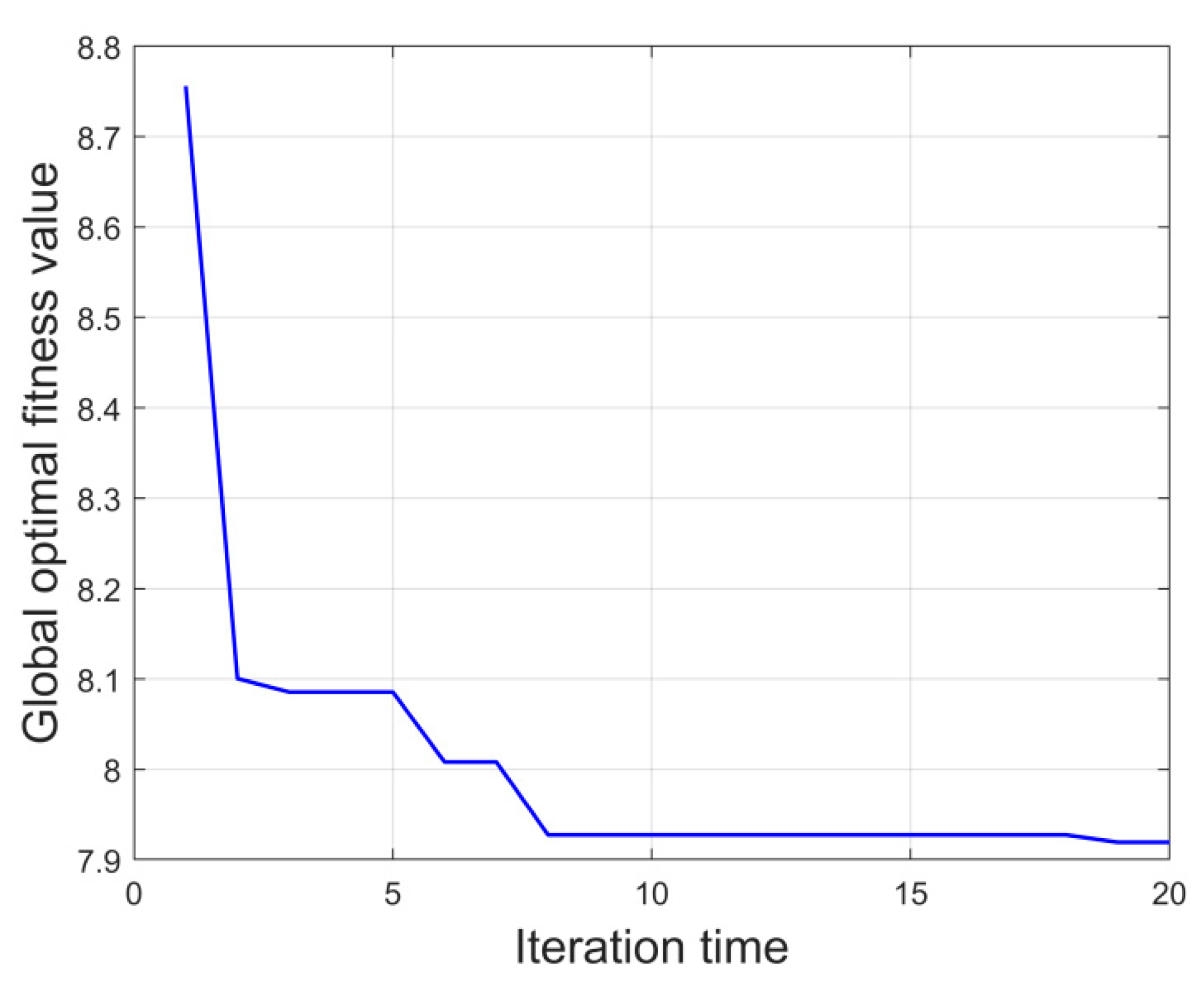
Step 4: The optimization is terminated when it reaches the maximum number of evolutions. Then the global best position is output, which is the target parameters of the controller. The convergence curve of optimal fitness value is also printed.
4.2. Optimization Experiments and Result Analysis
Here we conduct optimization of three control systems by using the HPSO algorithm mentioned above. To the SIFOFLC system, the particle dimension is four with the fractional order of the error signal and the scale factor of the depth controller and heading controller. We adopted the standard Oustaloup filter module deriving from FOTF toolbox [
29] to perform fractional derivative operator, the frequency band was set to [0.001,1000] and the filter order was 4. As for the FOPID control system, the dimension of particle is 10, so that each FOPID controller has five unknown parameters. For the T-S FLC control system, only two scale factors are to be optimized. The membership functions and fuzzy rules of T-S FLC were determined through empirical approach, and its control surface is shown in
Figure 6.
The coefficients of the HPSO algorithm are set as follows: the particle size is 10 and the maximum number of evolution is 20. The limit of the inertia weight,
, is set to between 1 and 0.7. The learning factors
and
are set as value 2, the social factor
is set as value 0.7 and the time interval coefficient
is set as value 0.5. The searching range for parameters are presented in
Appendix A. Furthermore, we implement multiple optimizations and adopt the optimal result to solve randomness.
Figure 10,
Figure 11 and
Figure 12 respectively show the convergence curve of optimal fitness of three control systems and the obtained target controller parameters are illustrated in
Table 3. It can be observed that all the curves tend to decline through evolution, which illustrates the effectiveness of optimization. Actually, the optimal fitness of three control systems respectively decreases by 19.8%, 37.9% and 9.6%. The FOPID controller clearly outperforms the other two controllers as it has the highest degrees of freedom. The optimization effect of the SIFOFLC system is twice as good as the T-S FLC system and its ultimate fitness is significantly less than the others. These results demonstrate that the introduction of a fractional differential operator not only increases degrees of freedom and the flexibility of the controller but also improves the control performance, as is particularly demonstrated in the next section.
5. Simulation and Analysis
In this section, we conduct comparative simulations to verify the effectiveness of the proposed SIFOFLC algorithm for AUV motion control. The optimized controllers expressed in
Table 3 are applied and the target trajectory of AUV does not change.
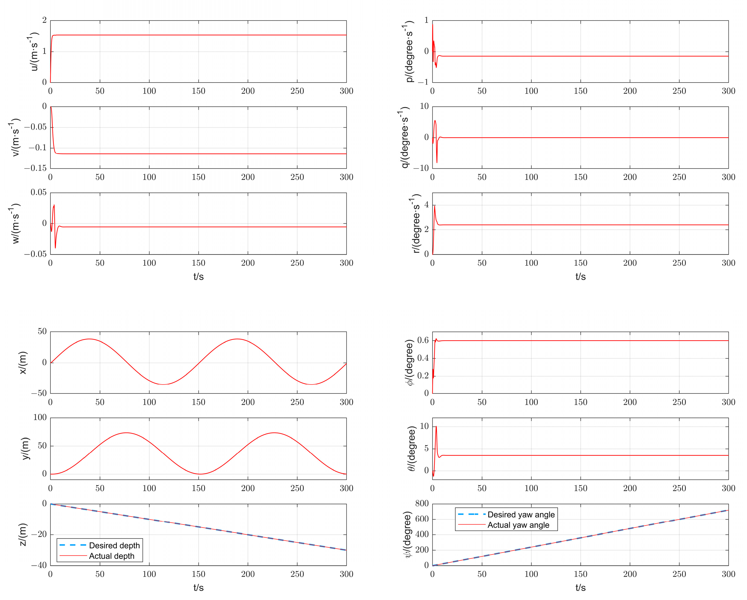
Figure 13 shows the trajectory of AUV under SIFOFLC and the state of the response is depicted in
Figure 14. Simulation results reveal that the trajectory tracking is accurate and rapid with SIFOFLC. Actually, the steady state error of depth is within 0.01 m in 6.5 s and gradually decreases to approximately 0.002 m in 7 s. Correspondingly, the maximum error of yaw angle is
and it gradually decreases to
in 13 s. The cruise speed maintains 1.54 m/s and the peak overshoot of pitch angle is
.
Figure 15 and
Figure 16 respectively illustrate the angular velocity of an AUV using FOPID controller and T-S FLC. Furthermore, the oscillation and settling times of angular velocity, the ITAE index of track error and the optimal fitness value are all presented in
Table 4. The responses with SIFOFLC algorithm have much shorter settling times and steady state errors. Compared with the SIFOFLC, the control performance obtained via the FOPID controller and T-S FLC requires a much longer settling time, and they also oscillate considerably in the beginning, which may lead to an unstable performance of the controlled system. Simulation results clearly reveal the superior stability and transient control performance of the proposed SIFOFLC.
6. Conclusions
In this study, we proposed a SIFOFLC algorithm for an AUV motion control system. Unlike a conventional FLC algorithm, this is reduced to a SISO controller by using the signed distance method, which provides a significant reduction to parameter tuning and computation burden. In addition, a fractional derivative operator was applied to increase degrees of freedom of the controller, hence the proposed control algorithm is more flexible and adaptive to the AUV motion control system. Furthermore, we developed an HPSO algorithm and applied it to optimize the controller parameters. The simulation results show that the proposed controller enhances the stability and transient performance of the controlled AUV motion system, which manifests in less oscillations of angular velocity, shorter dynamic settling time, and higher control accuracy. In future studies, we will perform experiments using the proposed controller to verify its practicability.

 ,
, 


