


Effects of Competition Intensities and R&D Spillovers on a Cournot Duopoly Game of Digital Economies

1
School of Business, Guangzhou College of Technology and Business, Guangzhou 510850, China
2
School of Applied Economics, Renmin University of China, Beijing 100872, China
*
Author to whom correspondence should be addressed.
Fractal Fract. 2023, 7(10), 737; https://0-doi-org.brum.beds.ac.uk/10.3390/fractalfract7100737
Submission received: 6 September 2023
/
Revised: 2 October 2023
/
Accepted: 4 October 2023
/
Published: 6 October 2023
(This article belongs to the Topic Advances in Nonlinear Dynamics: Methods and Applications)
Abstract
:In this paper, we introduce a Cournot duopoly game that can characterize fierce competition in digital economies and employ it to examine the effects of research and development (R&D) spillovers while considering various competition intensities. We obtain the analytical solution of the Nash equilibrium and the expression of commodity price, firm production, and variable profit under some key competition intensities. Furthermore, we analyze the local stability of the Nash equilibrium and derive that the equilibrium may lose its stability only through a 1:4 resonance bifurcation. Numerical simulations are conducted, through which we find that the Nash equilibrium transitions to complex dynamics through a cascade of period-doubling bifurcations. Phase portraits are also provided to illustrate more details of the dynamics, which confirm the previous theoretical finding that the Nash equilibrium loses its stability through a 1:4 resonance bifurcation.
1. Introduction
In this paper, we introduce a game that can be applied to characterizing competition in digital economies, especially in industries of digital products. In general, digital economies refer to economies where digital technologies are intensively used. Digital technologies are the representation of information in bits. In other words, in digital economies, information in all its forms becomes digital, is reduced to bits, and can be stored in devices. In comparison, in traditional economies, information is in physical forms such as cash, checks, invoices, reports, face-to-face meetings, maps, and photographs.
Digital products, also known as information goods, electronic information products, or virtual products, are conceptualized as bit-based objects distributed through electronic channels [1]. As pointed out by Goldfarb and Tucker [2], the main feature of digital goods is that certain costs fall substantially and perhaps approach zero. Compared to traditional products, digital goods possess much lower variable costs including, e.g., lower search costs, lower replication costs, lower transportation costs, lower tracking costs, and lower verification costs. Furthermore, Bertani et al. [3] pointed out that digital firms possess high R&D fixed costs compared to their variable costs since their products require deep know-how and a scarce quantity of resources. Accordingly, for digital economies, it is more appropriate to consider R&D costs as part of fixed costs rather than variable costs.
A duopoly refers to a market structure characterized by the presence of two firms that coexist and compete with each other. In contrast, within a market characterized by perfect competition, several small firms engage in competition with each other. The dynamics of duopolistic competition exhibit a higher level of complexity than those of perfect competition because participants in duopolistic markets are influenced by strategic decisions made by their rivals. It is widely acknowledged that Cournot [4] was the pioneer in developing the original theoretical framework for duopoly. The formulation of Cournot’s model is usually based on the assumptions of linear demand and costs. These assumptions allow us to represent the model using a linear map. In the context of duopolistic competition, the unique equilibrium of the linear model is globally stable. The utilization of Cournot games has been extensive across several domains, including international trade [5], e-commerce [6], and even biological processes [7].
In particular, the framework of Cournot games has also been applied to explore the effects of R&D spillovers on firms’ production and investment strategies. For example, d’Aspremont and Jacquemin [8] first introduced a simple yet elegant two-stage duopoly model to compare the cooperation and noncooperation behaviors in the R&D stage when spillovers are involved. They found that if the spillover effects are large enough, then cooperation in R&D increases both R&D expenditures and production quantities compared to noncooperative R&D. However, Henriques [9] pointed out that it is only meaningful to compare the cooperative and noncooperative solutions in the models of d’Aspremont and Jacquemin if these solutions are stable. Thus, Henriques [9] analyzed the local stability of the equilibrium and found that the result of d’Aspremont and Jacquemin [8] holds and introducing spillovers in the noncooperative model may increase the stability of the equilibrium. The literature related to R&D spillovers also includes, e.g., [10,11,12,13,14]. Symeonidis [12] compared the Cournot and Bertrand equilibria in R&D competition games and investigated the amounts of firms’ R&D investment, the quality and quantity of products, as well as the social welfare. Vives [13] explored the effects of competition on process and product innovation, where results are acquired for various market structures. The study of networks in economics has become popular recently. Accordingly, Bischi and Lamantia [10,11] introduced a two-stage oligopoly game where firms are arranged within networks. In their models, firms can cooperate with bilateral agreements to share knowledge and compete in the market.
For simplicity, researchers such as d’Aspremont and Jacquemin [8] tend to take the assumptions of linear demand and linear cost functions. However, various empirical studies in the existing literature do not support linear settings because nonlinearities were widely observed. For example, Ng [15] used threshold autoregressive models to study the price data of commodities and discovered evidence of nonlinearities in price. Adrangi and Chatrath [16] found strong evidence of nonlinear dependence and pointed out that the well-known ARCH-type processes may generally explain the nonlinearities in the data if the effects of seasonal and contract maturity are controlled. Accordingly, in this paper, we employ the isoelastic demand function, which is nonlinear and was first introduced by Puu [17] into the study of duopolistic competition. In addition, the assumption of nonlinear demand in oligopoly models may give rise to complex dynamics such as chaotic attractors. Many contributions have been made in the strand of nonlinear Cournot and Bertrand games. Readers may refer to, e.g., [18,19,20,21,22,23,24,25,26,27,28]. Notably, among them, Andaluz et al. [19] investigated a nonlinear Cournot oligopoly with N firms under the assumption of a more general isoelastic demand function and revealed that the effect of demand elasticity on the local stability depends on players’ adjustment mechanisms.
In this paper, we introduce a dynamic Cournot duopoly game of digital economies, where the market is supposed to be endowed with the isoelastic demand function. After that, we use this game to explore the effects of R&D spillovers by taking into account the competition intensity of the market. Compared to traditional economies, in specific development stages of digital economies, we may have an extremely high degree of market competition, which is due to the features of digital industries such as network effects, winner-take-all, and market lock-in (refer to [3] for additional information). Various empirical studies, e.g., [29,30,31], verify the existence of the business model of digital companies to suppress competitors at the expense of profits. This empirical finding can be explained with the different valuation methods of high-tech companies. For example, Demers and Lev [32] developed an empirical valuation model and found that some measures of Web traffic are value-relevant to the share prices of Internet companies, particularly those indicating reach (the percentage of a Web site’s visitors relative to the total Web-surfing population).
Our study is different from the current literature in the following three aspects. First, we suppose that players in our model are boundedly rational in the sense that each firm does not possess complete information regarding its rival’s competing strategies but naively conjectures its rival will produce the same output as the last period. This assumption of adjustment mechanisms is different from that of Bischi and Lamantia [33], where it is assumed that firms adjust their output according to gradient dynamics. Second, in addition to the effects of R&D spillovers, our study considers the effects of competition intensities on the dynamics of our model and the variation in several important economic variables. It is important to introduce the parameter controlling competition intensities into our game since a high degree of market competition is one of the typical characteristics of digital economies. The market structure with distinct competition intensities has been intensively studied by economists such as Matsumura et al. [34], Shibata [35], and Ishikawa and Shibata [36,37]. Third, unlike the model of d’Aspremont and Jacquemin [8], our model does not introduce the R&D investment variable but only focuses on the output variable of the involved firms. This setup of not introducing the R&D investment variable is borrowed from Bischi and Lamantia [33], Li et al. [38], and Zhou and Cui [39].
We solve the Nash equilibrium of our model analytically and examine the expression of commodity price, firm production, and variable profit under some key competition intensities. Furthermore, we analyze the local stability of the model and derive that the Nash equilibrium can lose its stability only through a 1:4 resonance bifurcation. Numerical simulations are conducted to investigate the effects of competition intensities and R&D spillovers on the dynamics of the game. Using one-dimensional and two-dimensional bifurcation diagrams, we observe that the Nash equilibrium bifurcates to a periodic solution, after which chaotic dynamics take place through a cascade of period-doubling bifurcations. Furthermore, it is also observed that the intermittence of periodic orbits between chaotic dynamics may appear. We also provide several phase portraits to illustrate more details of the dynamic transitions. In particular, these phase portraits confirm the theoretical finding that the Nash equilibrium is destabilized through a 1:4 resonance bifurcation.
The rest of this paper is structured as follows. Section 2 introduces the game setup, where the effects of competition intensities and R&D spillovers are considered. In Section 3, the equilibria of the model are solved in the closed form, and related economic variables at the Nash equilibrium are investigated. Section 4 explores the local stability of the Nash equilibrium and the nearby convergence factor. In Section 5, numerical simulations are conducted to study complex dynamic behaviors, e.g., periodic orbits and chaos, of our model. Section 6 concludes this paper.
2. Model Setup
Let us consider a market with two firms producing homogeneous products. We use and to represent the output quantity of firm 1 and firm 2, respectively. In real economies, the nonlinearity of the demand function can be widely observed (see, e.g., [15,16]). Accordingly, we assume that the market is featured via the isoelastic demand function employed by Puu [17], which is based on the hypothesis of the Cobb–Douglas utility function via the agents. Specifically, the market inverse demand function is of the form
where is the total market supply.
As mentioned by Goldfarb and Tucker [2], it requires a different emphasis rather than a fundamentally new economic theory to understand the effects of digital technology. Therefore, same as traditional economic models, the production cost of firm i is assumed to be linear, i.e., , where and are the fixed cost and marginal cost of firm i, respectively. Evidently, we have and . Goldfarb and Tucker [2] also stated that the main difference between digital economies and traditional economies is that certain costs of digital firms fall substantially and perhaps approach zero, including lower search costs, lower replication costs, lower transportation costs, lower tracking costs, and lower verification costs. In other words, the variable costs of digital economies are much lower. Similarly, Haltiwanger and Haltiwanger [40] pointed out that nondigital goods must be physically delivered to consumers, while digital goods can bypass the wholesale, retail, and transport networks; digital goods have very different pricing structures due to their high-fixed-cost and low-marginal-cost nature.
Bertani et al. [3] stated that the world related to the companies that produce digital technologies is totally different compared to the world that produces mass productions. In detail, diminishing returns can be used to characterize a mass production world, where products are heavily based on resources but lightly based on knowledge. In contrast, a knowledge-based world that produces digital goods can be characterized by increasing returns. Furthermore, these high-tech firms possess high R&D fixed costs compared to their variable production costs since their products require deep know-how and a scarce quantity of resources. Accordingly, for digital economies, it may be more appropriate to consider R&D costs as part of fixed costs rather than variable costs. Therefore, in our model, the above-mentioned high R&D fixed cost of firm i is assumed to be included in the fixed part of the production cost, i.e., .
Take the industry of Internet games in China as an example. There are two dominant game providers in China, namely, Tencent and NetEase, that compete with each other. Their fixed costs include office space costs, human resources costs, equipment costs, etc. However, their variable costs are mainly customer acquisition costs. The R&D costs are complex to calculate since an idea or innovation may be difficult to define. However, the salaries of all executives and employees who contributed to R&D obviously belong to the R&D costs, which include the chief technology officer (or any other technology or product-specific executives that were a part of the process), engineers, designers, external contractors, or consultants. Other R&D costs to consider include, e.g., the cloud infrastructure, version control services, and any other software or tools used to design and develop game products.
This paper focuses on R&D spillovers; thus, the positive cost externality must be considered. The positive cost externality can be explained as the cost reduction due to the presence of rivals, which may come from information exchanges on technological innovations, skilled workers, and R&D results. In the seminal work by d’Aspremont and Jacquemin [8], R&D spillovers are assumed to reduce the variable costs of products. This assumption is not applicable to digital goods because the R&D expenditures and thus the cost reduction due to spillovers should be counted in the fixed costs. As mentioned above, for digital goods, the R&D costs are mainly included in the fixed costs, but the costs of customer acquisition mainly constitute the variable costs that are hardly affected by spillovers. According to this special cost structure of digital goods, in our model, the cost reduction caused by spillovers is supposed to change only the fixed costs . We use to denote the coefficient of positive cost externality in the fixed costs of firm i related to the R&D spillovers of its rival. Specifically, if we consider the spillover effects, the fixed costs of producer i become , where represents the size of the competitor of firm i. The amplitude of is negatively related to the management level of firm i. The larger the value of , the greater the leakage of research results, or the greater the outflow of researchers of firm i, the lower the managerial ability of firm i. Furthermore, the larger the rival’s output (size), the more significant the R&D spillovers and the stronger the effects of lowering the fixed cost of firm i. It is reasonable to bound , which means that the effects of cost reduction are quite limited. This is because R&D spillovers can only reduce a company’s R&D expenditures (e.g., the salaries of some technical employees) to a certain extent. That is, the cost reduction due to spillovers is only a relatively small part of the fixed costs.
Moreover, additional costs should be paid by firm i to avoid its R&D spillovers (e.g., additional management expenditures to avoid the leakage of research results and higher salaries to prevent the outflow of researchers), which are positively related to the size of the firm (i.e., ) and negatively related to the positive cost externality coefficient (i.e., ). We denote the cost of avoiding spillovers as , where is the unit cost of controlling R&D spillovers. Thus, the total cost function of firm 1 is of the form
Similarly, the cost function of firm 2 should be
Here, we have for .
It should be mentioned that our cost functions are completely distinct from those employed by Bischi and Lamantia [33] due to the huge difference between the cost structures of digital and nondigital goods. The positive externality considered by Bischi and Lamantia [33] actually leads to a reduction in variable costs. However, this is not reasonable in digital economies since the variable costs of digital firms are mainly due to acquiring customers and can hardly be affected by R&D spillovers. Thus, we assume that R&D spillovers can only affect the fixed costs. Moreover, although Bischi and Lamantia [33] considered the extra cost paid by the firm to avoid spillovers, the cost of avoiding spillovers should be negatively related to the amplitude of R&D spillovers to the rivals, which is further related to the positive cost externality coefficients and . We consider these subtle relations in the setup of our cost functions.
Therefore, the profit of firm i is
To describe the effect of competition pressure, we assume that the operation objective of firm i is
where characterizes the competition intensity of the market. The objective function of this form may be traced back to [41,42]. Differently, Cyert and DeGroot [42] used it to discuss the cooperation between two companies and assumed that the coefficients of cooperation are negative and distinct. Afterward, Matsumura et al. [34] and Shibata [35] employed a similar payoff function to investigate the relationship between the competition degree of a market and the R&D expenditure. In their models, it is supposed that the parameter used to characterize the competition intensity is identical for different firms. Our model employs the same objective function as Matsumura et al. [34] and Shibata [35] to describe the competition intensity of the market.
In the special case of , we have , meaning that firm i only focuses on its own profits. One can see that . Accordingly, if , firm i makes decisions by not only considering its own profits but also gaining a comparative advantage over its rival. As indicated by Shibata [35], the case of corresponds to perfect competition, where no firms have market power. Furthermore, in specific development stages of digital industries, can be greater than one and even take large values. In this case, instead of marking profits (i.e., ), the operation goals of firms tend to include gaining a comparative advantage (i.e., ), suppressing competitors, capturing market share, and obtaining a monopolistic position in the market. Indeed, this can be widely observed in digital industries because digital economies are featured via network effects, winner-take-all, and market lock-in (refer to [3] for additional information).
The business model of suppressing competitors at the expense of profits is widespread in high-tech firms, which was confirmed by various empirical studies such as [29,30,31]. Denis and McKeon [29] pointed out that negative net cash flows have become much more pervasive, more persistent, and greater in magnitude since 1971 and firms with negative net cash flows recently tended to achieve cash balances through frequent equity offerings. In addition, it was revealed in [30,31] that the proportion of firms going public prior to achieving profitability has been increasing, which is driven by an increase in the proportion of high-tech firms. Indeed, these phenomena are related to the different valuation methods of high-tech companies. For example, Demers and Lev [32] developed an empirical valuation model and discovered that the reach and stickiness Web traffic performance measures were value-relevant to the share prices of Internet companies in 1999 and 2000.
Based on the above discussion, the first-order condition for firm 1 is
which is solved via the best-response reaction , where
Assume that period is the current period and period t is the last period. To maximize the objective function , firm 1 should choose its output at period according to
However, the above reaction requires that the player is completely rational. In the real world, however, a firm can hardly collect information on business secrets such as the production plan of its competitor. Thus, it is reasonable to assume the bounded rationality of firms in the sense that firms have no idea about rivals’ competing strategies but naively conjecture their rivals will produce the same output as the last period. Specifically, if firm 1 is boundedly rational, then it naively expects firm 2’s output at period to be . In practice, instead of (1), the reaction function of firm 1 is set to be
Similarly, the reaction function of firm 2 is
In short, the iteration map of our game can be described as
Remark 1.
In the setup of our game, we only select and to be the decision variables of the players. Unlike the model of d’Aspremont and Jacquemin [8], our model does not introduce the R&D investment variable but only treats the output as the endogenous decision. This setup of not introducing the R&D investment variable is borrowed from Bischi and Lamantia [33], Li et al. [38], and Zhou and Cui [39]. Furthermore, we assume the R&D expenditures are predetermined before the decisions of output. This assumption is appropriate as firms generally would not make R&D investment and output decisions simultaneously.
In the real world, the R&D expenditures (included in the fixed costs and ), the management levels (related to and ), and the competition intensities of the market (i.e., λ) may be decided by the involved firms and change over time. However, introducing , , and as decision variables into the model will result in a much greater complexity of the model and make analysis impossible. Instead, we assume that the values of , , and λ are somewhat fixed in a certain development stage of a digital industry and can be observed or computed from the market information. For example, we may divide the development of a digital company into three stages: the start-up stage, the fundraising and expansion stage, and the profitability stage. One can understand that at each stage, the fixed costs, the management level, and the operation objectives of a firm are relatively unchanged. In particular, the firm may tend to set its operational goals for the first and second stages as gaining market share at the expense of profits, namely, setting the value of λ much higher.
In what follows, readers will see that economically insightful implications can be discovered even by using this simplified game (2).
3. Nash Equilibrium
According to the iteration map (2), by setting and , we obtain the following equilibrium equations:
Then, we have
Consequently, it is acquired that
which implies
By plugging (4) back into one of the equilibrium Equation (3), we acquire two equilibria: the zero equilibrium and the Nash equilibrium
In what follows, we focus on the Nash equilibrium . An interesting exploration is to compute economic variables at the Nash equilibrium under some key competition intensities, e.g., . From (5), it is obtained that if , then
if , then
In particular, if , then . Thus, it is theoretically interesting that in the extremely competitive market () (this market exists only in theory), the output of firm 1 is related to the positive externality coefficient () rather than the marginal cost of production () and the cost of avoiding spillovers (). The output of firm 2 can be similarly analyzed.
Remark 2.
According to (4), we can derive some interesting results regarding the ratio . For example, provided that and , then if , meaning that less productive firms which produce less efficiently obtain smaller market shares. This is consistent with the allocation efficiency in an economy. Furthermore, if the competition intensity λ is large enough, we have that , which implies that if . Therefore, in a fiercely competitive environment, a higher management level of firm i (i.e., a smaller ) may lead to a larger market share (i.e., a larger ), which is consistent with our economic intuition.
At the Nash equilibrium, the price of the product is
One can see that if , then , namely, the sum of the cost of production without the positive externality and that of avoiding R&D spillovers. If , then
Furthermore, when approaches , the price is not related to the cost of production and that of avoiding spillovers, which approaches . That is, in a market of fierce competition, the product price is determined with the management level of firms. The higher the management level, the smaller the values of and and the lower the price.
The cost of firm 1 at the Nash equilibrium is complex, which is
Consequently, if , then
if , then
when , we have that
The variable profit V of a firm is usually defined to be the difference between its revenue and its variable cost. Accordingly, one can derive that if , then the variable profit of firm i is
Thus, the variable profit of firm 1 is always positive if the competition intensity is the lowest (), which is consistent with economic intuition. This is because, in this case, the involved companies operate to maximize their own profits and do not care about their competitors. However, when , we have that
From the above, one can see that the variable profit of firm 1 will be negative if . This means that firms in a market of extremely fierce competition () may sacrifice their positive variable profits to suppress competitors and capture the market if the sum of its marginal cost and its spillover-avoiding cost is high enough.
4. Local Stability and Convergence Factors
In this section, we analyze the local stability of the Nash equilibrium obtained in the above section and then explore the convergence speed of the trajectories near the equilibrium.
Theorem 1.
The Nash equilibrium is locally stable if
Proof.
The Jacobian matrix is
Accordingly, the characteristic equation is
It is easy to check that the signs of the two expressions in parentheses on the right-hand side of (8) are opposites. Thus, we obtain two conjugate imaginary eigenvalues
The Nash equilibrium is locally stable if both and hold. One can verify that this is equivalent to
which can be solved via (6). The proof is completed. □
Remark 3.
According to the classic bifurcation theory, the Nash equilibrium may lose its stability through a 1:4 resonance bifurcation when , which will be confirmed through numerical simulations in the next section.
In the following, we discuss the convergence speed of trajectories around the Nash equilibrium. For a one-dimensional iteration map , we define the convergence factor to be
where is the derivative and is the involved equilibrium of the map. However, for an n-dimensional iteration map with , the convergence factor is usually defined to be the spectral radius of its Jacobian matrix J at the considered equilibrium , i.e.,
where are the eigenvalues of . By definition, for any state sufficiently close to the equilibrium , it is known that
Therefore, the convergence factor characterizes the convergence speed in the sense that its reciprocal reflects the amplitude of the convergence speed. If , then successive states will approach the considered equilibrium as the evolution of the dynamic system. The smaller the convergence factor is, the faster a trajectory converges to the equilibrium. Particularly, if , the convergence speed is called to be super-linear.
Thus, for our model, we have that
i.e.,
Accordingly, the convergence speed is super-linear if and only if .
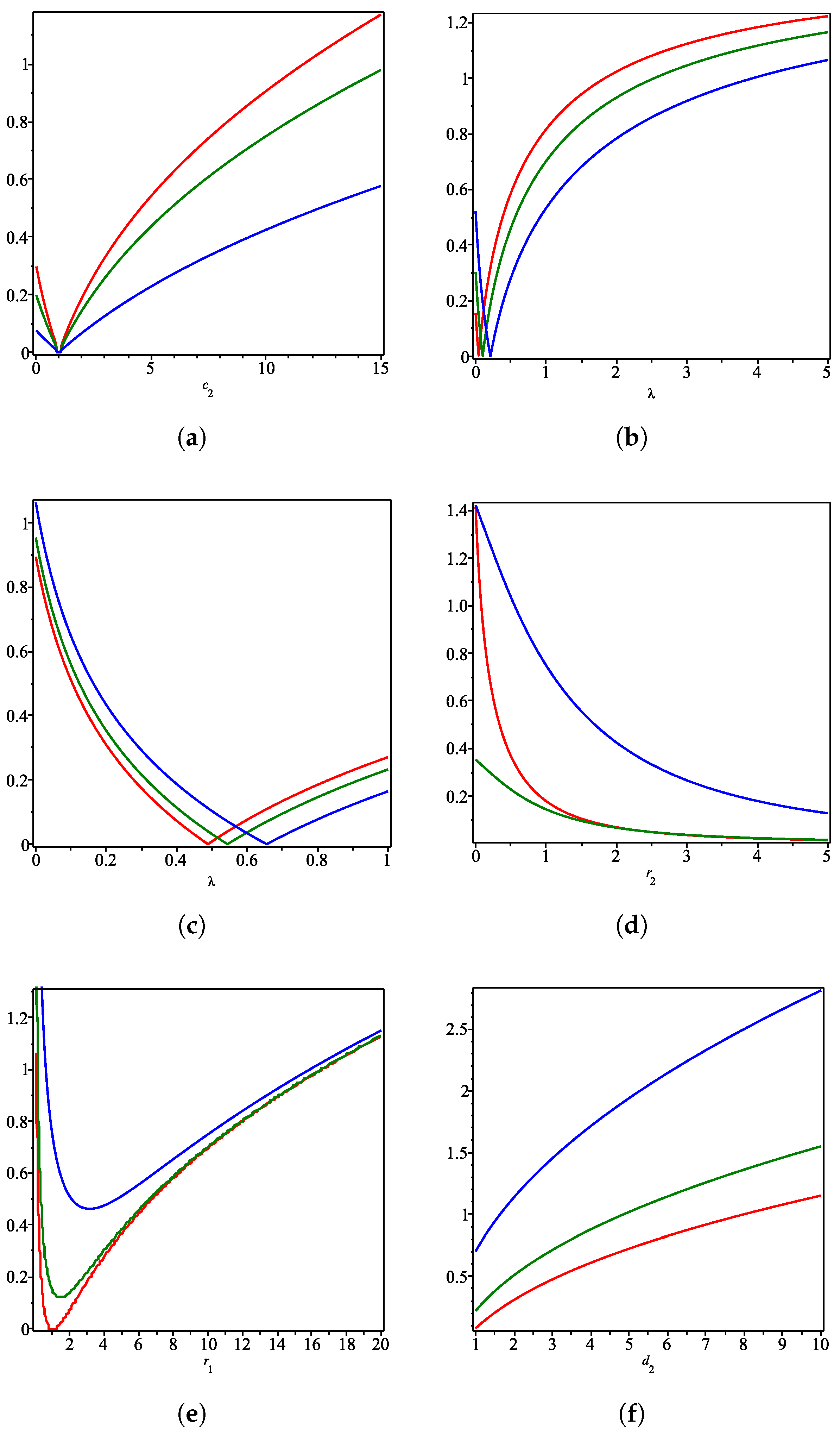
In what follows, some interesting cases are plotted in Figure 1 to illustrate the influences of the parameters on the convergence factors. For example, in Figure 1a, we set , , , , and . One can see that the convergence factor increases as the difference between and increases. In particular, when , the convergence factor vanishes, namely, the convergence speed becomes super-linear.
From Theorem 1, we conclude that if and are close enough to each other (precisely, ), the Nash equilibrium will become locally stable if is large enough. This conclusion is confirmed with Figure 1a, where . It is observed that the blue curve () is lower than the green () and red () ones. That is to say, in the case of , an increase in leads to an increase in the convergence speed and consequently makes the Nash equilibrium more stable. From an economic point of view, if the percentages of leakage of research results and that of outflow of researchers are close to each other (i.e., are are close) for two firms in the same digital industry, a more competitive environment will lead to the greater stability of the economic system. This fact may be explained with a cross-sectional comparison of different industries: the more competitive the industry, the more obvious the winner-takes-all effect and the less unstable the market.
However, increasing may destabilize the Nash equilibrium if and are sufficiently distinct. This fact is illustrated in Figure 1b, where we set , , , , and . It is observed that all three curves take values higher than 1 when because the ratio of to is large. If the value of approaches , then the left-hand side of (6) will approach . Thus, the Nash equilibrium may lose its local stability if the value of is sufficiently large and and are sufficiently distinct, meaning that the existence of firms with quite different managerial abilities in a fiercely competitive market may result in unstable outcomes.
Figure 1c reports that a decrease in the competition intensity may also destabilize the Nash equilibrium when the and are sufficiently different. In Figure 1c, we fix , , , , and but vary . The blue curve () will take values larger than one if approaches zero. This case is theoretically interesting and may not really exist because and seem to be close in the real market.
In Figure 1d, we explore this case by setting , , , , and . The red, green, and blue curves correspond to , 2, and 10, respectively. One can see that the convergence factor may be greater than one when the identical cost externality coefficient () approaches zero if the difference between and is large enough (see the red and blue curves). However, this is incorrect if and are close (see the green curve).
In contrast to Figure 1d, Figure 1e explores the case of , where we fix , , , and but vary . The red, green, and blue curves correspond to , 2, and 10, respectively. It is found that the Nash equilibrium may be destabilized if the value of is sufficiently large or sufficiently small compared to . Figure 1f investigates the influence of on the convergence speed if we fix other parameters. It is observed that if is large enough compared to , then the convergence factor will be greater than one.
Let be of moderate size. One can see that, if the difference between and , and , and and is small enough, then the Nash equilibrium of our game will be locally stable. We should mention that this fact can also be deduced by analyzing the stability condition (6). In real digital economies, and should be close to each other because the cost of customer acquisition should be about the same for different firms in the same industry. Moreover, the values of and are also close to each other since the cost of avoiding the leakage of research results and the per capita cost of preventing the outflow of researchers should not be much different for distinct firms. However, a huge difference in the management level of the firms may lead to a huge difference in the percentage of research leakage or the percentage of outflow of researchers. Therefore, the parameters and may take quite distinct values. This means that a large difference in the management level of companies in digital industries may be the main reason for the instability of the market.
5. Numerical Simulations
In this section, numerical simulations are conducted to investigate the complex dynamics of the duopoly game considered in this paper.
First, let us investigate the effects of the competition intensity and the positive cost externality coefficients on the dynamic behaviors of our model. For simplicity, we assume that the positive cost externality coefficients are identical, namely, . Figure 2a,b depict the bifurcation diagrams of the iteration map (2) with respect to and r, respectively, where , , and are set. In Figure 2a, we vary and fix . However, in Figure 2b, we vary and fix . The iterations start from the initial state . The diagrams against and are colored in red and blue, respectively, where periodic solutions with different orders and strange attractors can be observed. Furthermore, we find the route to chaos through a series of period-doubling bifurcations as or r decrease.
Figure 3 depicts two-dimensional bifurcation diagrams to show more complex dynamics with respect to the two parameters and r (). Readers can refer to [43] for additional details regarding two-dimensional bifurcation diagrams. In the numerical simulations producing the two-dimensional bifurcation diagrams, we fix the parameters , , and . Same as above, we set the initial state to be . Parameter points corresponding to periodic orbits with different orders are marked in different colors and are marked in yellow if the order is greater than 24 or the trajectory diverges (approaches ∞). In other words, the yellow points may be viewed as the parameter values where complex dynamics such as chaos take place. Figure 3a,b are given to display the panoramic and localized parameter windows, i.e., and , respectively. From Figure 3a,b, we find a series of period-doubling bifurcations, through which the Nash equilibrium loses its stability. In detail, the equilibrium first bifurcates to a two-cycle of () if we fix the value of and reduce the value of r. As r further decreases, one can observe a cascade of period-doubling bifurcations from the two-cycle orbit. Finally, chaotic dynamics appear when r is small enough.
Furthermore, we depict the phase portraits in Figure 4 by fixing the parameters , , , and and choosing to be the initial state. We plot the trajectory of 5000 iterations. From Figure 4a, it is observed that the trajectory converges to the Nash equilibrium when . If decreases and equals (see Figure 4b), then the trajectory also approaches the Nash equilibrium, but the convergence speed becomes much slower. These observations confirm the finding, given in Remark 3, that the Nash equilibrium loses its stability through a 1:4 resonance bifurcation. In Figure 4c, one can discover that a four-cycle orbit appears when and the amplitude of this periodic solution becomes larger as further decreases. In Figure 4d, the trajectory seems messy, but indeed a 16-cycle orbit can be found if we discard the first, e.g., 2000 iteration points. When , we observe a chaotic attractor with 16 pieces (see Figure 4e). If the value of becomes smaller and equals (see Figure 4f), it is found that the number of pieces of the chaotic attractor is reduced by half and becomes eight. Then, Figure 4g shows that a periodic orbit with order 32 reappears when . From Figure 4h, one can see that the dynamics of the system become chaotic again and there is a strange attractor with only four pieces when . Moreover, observations on Figure 4i reveal that there exists a periodic orbit with order 12 when . From Figure 4j,k, we discover that a chaotic attractor with four pieces reappears and the gaps between these pieces become smaller as the value of decreases. Finally, a chaotic attractor with one unique piece emerges when , as shown in Figure 4i.
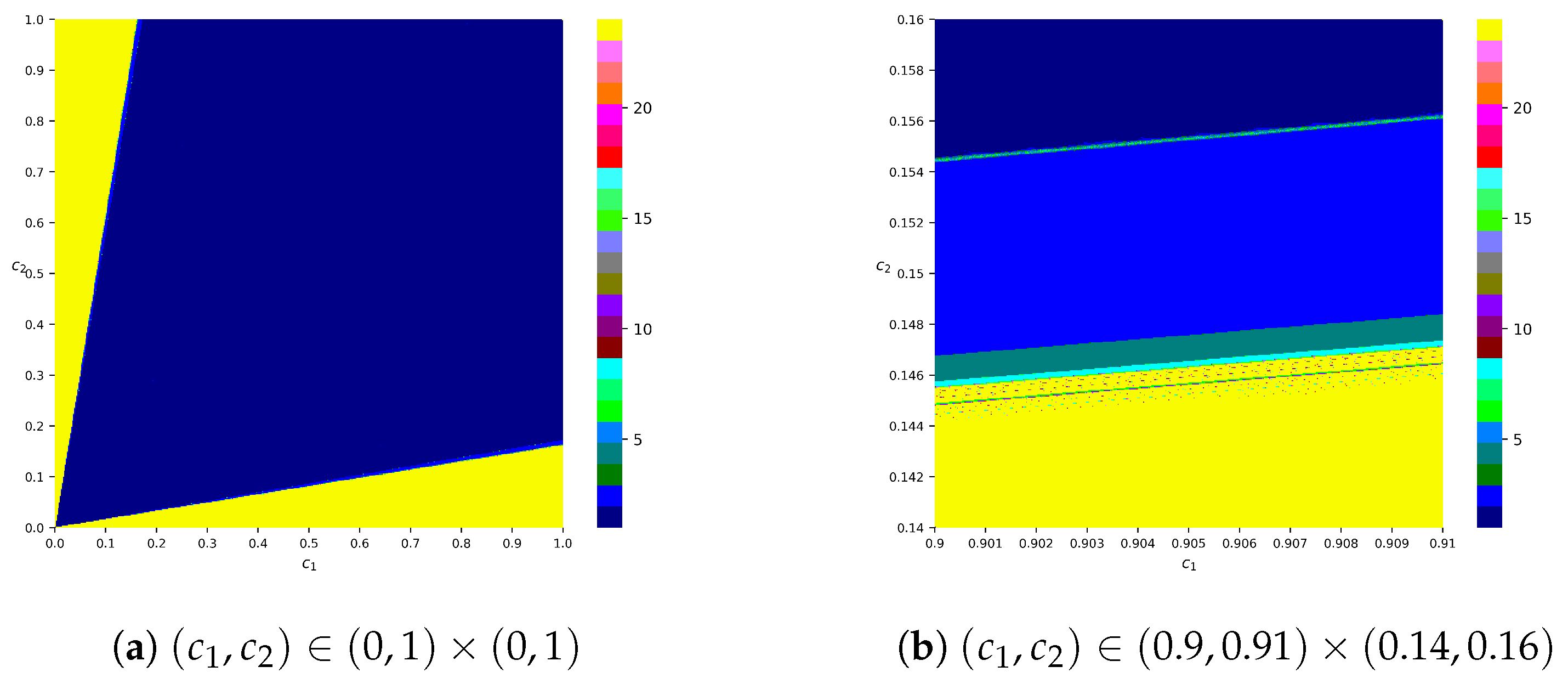
As stated at the end of the previous section, the parameters and ( and ) should take values close to each other in real digital economies. However, the values of and may be quite distinct because a huge difference in the management level of firms may lead to a huge difference in the percentage of research leakage or researcher outflow of firms. Accordingly, it is necessary to conduct numerical simulations to explore the influences of and on the dynamic behaviors of the duopoly game considered in this paper. In Figure 5, we plot the two-dimensional bifurcation diagram with respect to and by fixing the parameters , , and . Still, the initial state of the iterations is set to be . Similar to Figure 3, we use different colors to mark parameter points corresponding to periodic orbits with different orders. In particular, parameter points are marked in yellow if the order is greater than 24 or the trajectory diverges (approaches ∞). We observe that the trajectory will converge to a stable equilibrium if the parameter point lies not far away from the diagonal, i.e., , which is consistent with the results obtained in the previous section. However, one can see that if the difference between and is large, periodic solutions of order two, four, or higher and even chaotic trajectories may appear, meaning that a large difference in the management level of firms might result in complex phenomena such as periodic orbits and chaos in digital economies.
Furthermore, Figure 6 depicts the one-dimensional bifurcation diagram with respect to via fixing the parameters , , , and . The diagrams against and are colored in red and blue, respectively. More details of the dynamic transitions to complicated dynamics can be observed. One can see that the trajectory approaches the Nash equilibrium if is small enough. As the value of increases, a two-cycle orbit of () appears and then transitions to complex dynamics through a cascade of period-doubling bifurcations. However, if we further increase the value of , the trajectory will become simple once more and approach the Nash equilibrium.
For the sake of completeness, Figure 7 reports the two-dimensional bifurcation diagrams with respect to the cost parameters and although the cost parameters are not the focus of our study. Panoramic () and localized () views are displayed in Figure 7a,b, respectively. The transitions to chaotic dynamics can be observed in both views. One can see that the equilibrium loses its stability as the difference between and becomes large enough. Figure 7b depicts the transitions between different types of periodic orbits. According to Figure 7b, the equilibrium bifurcates to a two-cycle of () as the value of decreases if we fix . Then, transitions to chaos from this two-cycle orbit through a cascade of period-doubling bifurcations can be discovered. Furthermore, we also find the intermittence of periodic orbits between chaotic dynamics.
At the end, we try to explain the dynamic behaviors of the duopoly found in our numerical simulations from an economic point of view. As mentioned above, periodic solutions may take place in the duopoly game considered in this paper as we vary the involved parameters. In an economic system, periodic solutions are interesting because a boundedly rational firm cannot learn the pattern behind output and profits if a long period of periodic dynamics takes place. Furthermore, one can see that chaos may also appear in the model. If chaos appears, the pattern behind output and profits is nearly impossible to learn even for completely rational players. Therefore, it is extremely hard for a firm to handle a chaotic economy, where no market rules can be discovered and followed. The observations on chaotic dynamics in our numerical simulations are consistent with empirical validations of chaos in the literature. For example, the existence of low-dimensional chaos was identified by evidence in various markets such as the US crude oil market [44], the gold and silver market [45], and the soybean futures market [46]. We know that chaotic attractors are fractal sets since at small scales a chaotic attractor is approximately the Cartesian product of a Cantor set and a line segment; thus, it is roughly self-similar and has a box dimension that is not an integer. Fractal patterns are quite common as nature is full of fractals. Here, we can conclude that fractal patterns are widespread in economic systems, which are discovered from not only our numerical simulations but also various empirical studies.
6. Concluding Remarks
In this paper, we introduced a dynamic Cournot duopoly game of digital economies, where an isoelastic (nonlinear) demand function features the market. The nonlinear demand function is employed in our model since many empirical studies, including [15,16], rejected the linear assumption. Furthermore, the cost functions of our model were built on the special cost structure of digital goods. After that, we applied this duopoly game to explore the effects of R&D spillovers by considering various competition intensities of the market.
We investigated the game in detail, solved the Nash equilibrium analytically, and analyzed the expression of commodity price, firm output, and variable profit under several key competition intensities. Moreover, we investigated the local stability of the Nash equilibrium and introduced the convergence factor, the reciprocal of which reflects the amplitude of the convergence speed. In addition, according to bifurcation theory, we derived that the Nash equilibrium may lose its local stability through a 1:4 resonance bifurcation.
We conducted numerical simulations on the model and investigated the effects of the involved parameters on the dynamic transitions. Firstly, we assume that for the sake of simplicity in the investigation of the effects of the competition intensities and R&D spillovers. By using one-dimensional and two-dimensional bifurcation diagrams, we found that the Nash equilibrium can be destabilized as or r decreases. In real digital economies, the values of and may be quite distinct, but the parameters and ( and ) seem to take values close to each other. Therefore, our numerical simulations then focused on this situation by exploring the dynamic transitions of the model with respect to and . We observed that the Nash equilibrium bifurcates to a periodic solution, after which chaotic dynamics take place through a cascade of period-doubling bifurcations. It was also observed that an intermittence of periodic orbits between chaotic dynamics may appear. In addition, phase portraits were provided to illustrate more details of the dynamic transitions with respect to . Through these phase portraits, we confirmed the previous theoretical finding that the Nash equilibrium can be destabilized through a 1:4 resonance bifurcation.
Author Contributions
Conceptualization, X.L.; methodology, X.L.; validation, X.L. and L.S.; formal analysis, X.L.; investigation, X.L., J.W. and L.S.; writing—original draft preparation, X.L. and J.W.; writing—review and editing, X.L., J.W. and L.S. All authors have read and agreed to the published version of the manuscript.
Funding
This research was funded by the Philosophy and Social Science Foundation of Guangdong under Grant GD21CLJ01 and Guangdong Education Research Project under Grant 2022GXJK432.
Data Availability Statement
Not applicable.
Acknowledgments
The authors are grateful to the anonymous referees for their helpful comments.
Conflicts of Interest
The authors declare no conflict of interest.
References
- Koiso-Kanttila, N. Digital content marketing: A literature synthesis. J. Mark. Manag. 2004, 20, 45–65. [Google Scholar] [CrossRef]
- Goldfarb, A.; Tucker, C. Digital economics. J. Econ. Lit. 2019, 57, 3–43. [Google Scholar] [CrossRef]
- Bertani, F.; Ponta, L.; Raberto, M.; Teglio, A.; Cincotti, S. The complexity of the intangible digital economy: An agent-based model. J. Bus. Res. 2021, 129, 527–540. [Google Scholar] [CrossRef]
- Cournot, A.A. Recherches sur les Principes Mathématiques de la Théorie des Richesses; chez L. Hachette: Paris, France, 1838. [Google Scholar]
- Xin, B.; Zhang, M. Evolutionary game on international energy trade under the Russia-Ukraine conflict. Energy Econ. 2023, 125, 106827. [Google Scholar] [CrossRef]
- Zhang, M.; Fu, Y.; Zhao, Z.; Pratap, S.; Huang, G.Q. Game theoretic analysis of horizontal carrier coordination with revenue sharing in E-commerce logistics. Int. J. Prod. Res. 2019, 57, 1524–1551. [Google Scholar] [CrossRef]
- Guirao, J.L.G.; Rubio, R.G. Detecting simple dynamics in Cournot-like models. J. Comput. Appl. Math. 2009, 233, 1091–1095. [Google Scholar] [CrossRef]
- D’Aspremont, C.; Jacquemin, A. Cooperative and noncooperative R&D in duopoly with spillovers. Am. Econ. Rev. 1988, 78, 1133–1137. [Google Scholar]
- Henriques, I. Cooperative and noncooperative R&D in duopoly with spillovers: Comment. Am. Econ. Rev. 1990, 80, 638–640. [Google Scholar]
- Bischi, G.I.; Lamantia, F. A dynamic model of oligopoly with R&D externalities along networks. Part I. Math. Comput. Simul. 2012, 84, 51–65. [Google Scholar] [CrossRef]
- Bischi, G.I.; Lamantia, F. A dynamic model of oligopoly with R&D externalities along networks. Part II. Math. Comput. Simul. 2012, 84, 66–82. [Google Scholar] [CrossRef]
- Symeonidis, G. Comparing Cournot and Bertrand equilibria in a differentiated duopoly with product R&D. Int. J. Ind. Organ. 2003, 21, 39–55. [Google Scholar] [CrossRef]
- Vives, X. Innovation and competitive pressure. J. Ind. Econ. 2008, 56, 419–469. [Google Scholar] [CrossRef]
- Zhou, W.; Liu, H. Complexity analysis of dynamic R&D competition between high-tech firms. Commun. Nonlinear Sci. Numer. Simul. 2023, 118, 107029. [Google Scholar] [CrossRef]
- Ng, S. Looking for evidence of speculative stockholding in commodity markets. J. Econ. Dyn. Control 1996, 20, 123–143. [Google Scholar] [CrossRef]
- Adrangi, B.; Chatrath, A. Non-linear dynamics in futures prices: Evidence from the coffee, sugar and cocoa exchange. Appl. Financ. Econ. 2003, 13, 245–256. [Google Scholar] [CrossRef]
- Puu, T. Chaos in duopoly pricing. Chaos Solitons Fractals 1991, 1, 573–581. [Google Scholar] [CrossRef]
- Ahmed, E.; Elsadany, A.A.; Puu, T. On Bertrand duopoly game with differentiated goods. Appl. Math. Comput. 2015, 251, 169–179. [Google Scholar] [CrossRef]
- Andaluz, J.; Elsadany, A.A.; Jarne, G. Dynamic Cournot oligopoly game based on general isoelastic demand. Nonlinear Dyn. 2020, 99, 1053–1063. [Google Scholar] [CrossRef]
- Askar, S. Local and global analysis of a nonlinear duopoly game with heterogeneous firms. Adv. Differ. Equ. 2020, 2020, 682. [Google Scholar] [CrossRef]
- Cavalli, F.; Naimzada, A.; Tramontana, F. Nonlinear dynamics and global analysis of a heterogeneous Cournot duopoly with a local monopolistic approach versus a gradient rule with endogenous reactivity. Commun. Nonlinear Sci. Numer. Simul. 2015, 23, 245–262. [Google Scholar] [CrossRef]
- Elabbasy, E.; Agiza, H.; Elsadany, A. Analysis of nonlinear triopoly game with heterogeneous players. Comput. Math. Appl. 2009, 57, 488–499. [Google Scholar] [CrossRef]
- Kopel, M. Simple and complex adjustment dynamics in Cournot duopoly models. Chaos Solitons Fractals 1996, 7, 2031–2048. [Google Scholar] [CrossRef]
- Li, X.; Fu, J.; Niu, W. Complex dynamics of knowledgeable monopoly models with gradient mechanisms. Nonlinear Dyn. 2023, 111, 11629–11654. [Google Scholar] [CrossRef]
- Li, X.; Su, L. A heterogeneous duopoly game under an isoelastic demand and diseconomies of scale. Fractal Fract. 2022, 6, 459. [Google Scholar] [CrossRef]
- Ma, J.; Wang, Z. Optimal pricing and complex analysis for low-carbon apparel supply chains. Appl. Math. Model. 2022, 111, 610–629. [Google Scholar] [CrossRef]
- Matsumoto, A.; Nonaka, Y.; Szidarovszky, F. Nonlinear dynamics and adjunct profits in two boundedly rational models of monopoly. Commun. Nonlinear Sci. Numer. Simul. 2022, 116, 106868. [Google Scholar] [CrossRef]
- Puu, T. The chaotic monopolist. Chaos Solitons Fractals 1995, 5, 35–44. [Google Scholar] [CrossRef]
- Denis, D.J.; McKeon, S.B. Persistent negative cash flows, staged financing, and the stockpiling of cash balances. J. Financ. Econ. 2021, 142, 293–313. [Google Scholar] [CrossRef]
- Jain, B.A.; Jayaraman, N.; Kini, O. The path-to-profitability of Internet IPO firms. J. Bus. Ventur. 2008, 23, 165–194. [Google Scholar] [CrossRef]
- Ritter, J.R.; Welch, I. A review of IPO activity, pricing, and allocations. J. Financ. 2002, 57, 1795–1828. [Google Scholar] [CrossRef]
- Demers, E.; Lev, B. A rude awakening: Internet shakeout in 2000. Rev. Account. Stud. 2001, 6, 331–359. [Google Scholar] [CrossRef]
- Bischi, G.I.; Lamantia, F. Nonlinear duopoly games with positive cost externalities due to spillover effects. Chaos Solitons Fractals 2002, 13, 701–721. [Google Scholar] [CrossRef]
- Matsumura, T.; Matsushima, N.; Cato, S. Competitiveness and R&D competition revisited. Econ. Model. 2013, 31, 541–547. [Google Scholar] [CrossRef]
- Shibata, T. Market structure and R&D investment spillovers. Econ. Model. 2014, 43, 321–329. [Google Scholar]
- Ishikawa, N.; Shibata, T. Market competition, R&D spillovers, and firms’ cost asymmetry. Econ. Innov. New Technol. 2020, 29, 847–865. [Google Scholar] [CrossRef]
- Ishikawa, N.; Shibata, T. R&D competition and cooperation with asymmetric spillovers in an oligopoly market. Int. Rev. Econ. Financ. 2021, 72, 624–642. [Google Scholar] [CrossRef]
- Li, H.; Zhou, W.; Elsadany, A.A.; Chu, T. Stability, multi-stability and instability in Cournot duopoly game with knowledge spillover effects and relative profit maximization. Chaos Solitons Fractals 2021, 146, 110936. [Google Scholar] [CrossRef]
- Zhou, W.; Cui, M. Synchronization and global dynamics of a Cournot model with nonlinear demand and R&D spillovers. Int. J. Bifurc. Chaos 2021, 31, 2150209. [Google Scholar]
- Haltiwanger, J.; Jarmin, R.S. Measuring the digital economy. In Understanding the Digital Economy: Data, Tools and Research; MIT Press: Cambridge, UK, 2000; pp. 13–33. [Google Scholar]
- Bowley, A.L. The Mathematical Roundwork of Economics: An Introductory Treatise; Clarendon Press: Oxford, UK, 1924. [Google Scholar]
- Cyert, R.M.; DeGroot, M.H. An analysis of cooperation and learning in a duopoly context. Am. Econ. Rev. 1973, 63, 24–37. [Google Scholar]
- Li, X.; Li, B.; Liu, L. Stability and dynamic behaviors of a limited monopoly with a gradient adjustment mechanism. Chaos Solitons Fractals 2023, 168, 113106. [Google Scholar] [CrossRef]
- Lichtenberg, A.J.; Ujihara, A. Application of nonlinear mapping theory to commodity price fluctuatuions. J. Econ. Dyn. Control 1989, 13, 225–246. [Google Scholar] [CrossRef]
- Frank, M.; Stengos, T. Measuring the strangeness of gold and silver rates of return. Rev. Econ. Stud. 1989, 56, 553–567. [Google Scholar] [CrossRef]
- Blank, S.C. “Chaos” in futures markets? A nonlinear dynamical analysis. J. Futur. Mark. 1991, 11, 711–728. [Google Scholar] [CrossRef]
Figure 1.
Convergence factor as the parameters vary. (a) Fix , , , , and , but vary . The red, green, and blue curves are corresponding to , 1, and 5, respectively. (b) Fix , , , , and , but vary . The red, green, and blue curves are corresponding to , 1, and 2, respectively. (c) Fix , , , , and , but vary . The red, green, and blue curves are corresponding to , 1, and 2, respectively. (d) Fix , , , and with . The red, green, and blue curves are corresponding to , 2, and 10, respectively. (e) Fix , , , , and , but vary . The red, green, and blue curves are corresponding to , 2, and 10, respectively. (f) Fix , , , , and , but vary . The red, green, and blue curves are corresponding to , , and , respectively.

Figure 2.
Let . The one-dimensional bifurcation diagrams with respect to and r via fixing the parameters , , and . We choose to be the initial state of the iterations. The diagrams against and are colored in red and blue, respectively.
Figure 2.
Let . The one-dimensional bifurcation diagrams with respect to and r via fixing the parameters , , and . We choose to be the initial state of the iterations. The diagrams against and are colored in red and blue, respectively.

Figure 3.
Let . The two-dimensional bifurcation diagram with respect to and r via fixing the parameters , , and . We choose to be the initial state of the iterations. Parameter points corresponding to periodic orbits with different orders are marked in different colors and are marked in yellow if the order is greater than 24 or the trajectory diverges (approaches ∞).

Figure 4.
The phase portraits of the duopoly via fixing the parameters , , , and . We choose to be the initial state of the iterations.
Figure 4.
The phase portraits of the duopoly via fixing the parameters , , , and . We choose to be the initial state of the iterations.

Figure 5.
The two-dimensional bifurcation diagram with respect to and via fixing the parameters , , and . We choose to be the initial state of the iterations. Parameter points corresponding to periodic orbits with different orders are marked in different colors and are marked in yellow if the order is greater than 24 or the trajectory diverges (approaches ∞).

Figure 6.
The one-dimensional bifurcation diagram with respect to . We fix the other parameters , , , and and choose to be the initial state of the iterations. The diagrams against and are colored in red and blue, respectively.
Figure 6.
The one-dimensional bifurcation diagram with respect to . We fix the other parameters , , , and and choose to be the initial state of the iterations. The diagrams against and are colored in red and blue, respectively.

Figure 7.
The two-dimensional bifurcation diagram with respect to and via fixing the parameters , , and . We choose to be the initial state of the iterations. Parameter points corresponding to periodic orbits with different orders are marked in different colors and are marked in yellow if the order is greater than 24 or the trajectory diverges (approaches ∞).

Disclaimer/Publisher’s Note: The statements, opinions and data contained in all publications are solely those of the individual author(s) and contributor(s) and not of MDPI and/or the editor(s). MDPI and/or the editor(s) disclaim responsibility for any injury to people or property resulting from any ideas, methods, instructions or products referred to in the content. |
© 2023 by the authors. Licensee MDPI, Basel, Switzerland. This article is an open access article distributed under the terms and conditions of the Creative Commons Attribution (CC BY) license (https://creativecommons.org/licenses/by/4.0/).
Share and Cite
MDPI and ACS Style
Li, X.; Su, L.; Wang, J. Effects of Competition Intensities and R&D Spillovers on a Cournot Duopoly Game of Digital Economies. Fractal Fract. 2023, 7, 737. https://0-doi-org.brum.beds.ac.uk/10.3390/fractalfract7100737
AMA Style
Li X, Su L, Wang J. Effects of Competition Intensities and R&D Spillovers on a Cournot Duopoly Game of Digital Economies. Fractal and Fractional. 2023; 7(10):737. https://0-doi-org.brum.beds.ac.uk/10.3390/fractalfract7100737
Chicago/Turabian StyleLi, Xiaoliang, Li Su, and Jianjun Wang. 2023. "Effects of Competition Intensities and R&D Spillovers on a Cournot Duopoly Game of Digital Economies" Fractal and Fractional 7, no. 10: 737. https://0-doi-org.brum.beds.ac.uk/10.3390/fractalfract7100737