
On q-Hermite–Hadamard Type Inequalities via s-Convexity and (α,m)-Convexity

1
Department of Mathematics, Politehnica University of Timisoara, 300006 Timisoara, Romania
2
Department of Management, Politehnica University of Timisoara, 300006 Timisoara, Romania
*
Author to whom correspondence should be addressed.
Fractal Fract. 2024, 8(1), 12; https://0-doi-org.brum.beds.ac.uk/10.3390/fractalfract8010012
Submission received: 24 November 2023
/
Revised: 17 December 2023
/
Accepted: 19 December 2023
/
Published: 22 December 2023
(This article belongs to the Special Issue Fractional Integral Inequalities and Applications, 2nd Edition)
Abstract
:The purpose of the paper is to present new q-parametrized Hermite–Hadamard-like type integral inequalities for functions whose third quantum derivatives in absolute values are s-convex and -convex, respectively. Two new q-integral identities are presented for three time q-differentiable functions. These lemmas are used like basic elements in our proofs, along with several important tools like q-power mean inequality, and q-Holder’s inequality. In a special case, a non-trivial example is considered for a specific parameter and this case illustrates the investigated results. We make links between these findings and several previous discoveries from the literature.
1. Introduction
The q-calculus is used today in a lot of mathematical areas, like combinatorics, orthogonal polynomials, number theory, mechanics and theory of relativity, and basic hypergeometric functions, and this field started with the work of Jackson [1,2]. It has the advantage of substituting the classical derivative with a difference operator in order to more easily manipulate the sets of non-differentiable mappings. In recent times, Q-calculus has gained increasing importance in some fields of science, like geometry function theory, statistics, quantum mechanics, and also, particle physics, cosmology, and economic geology.
Two fundamental publications on quantum-calculus were written by Ernst [3], and Kac and Cheung [4]. Ntouyas and Tariboon in [5,6] analyzed q-derivatives and q-integrals across intervals like establishing many q-analogues for the well-known Holder, Ostrowski, Hermite–Hadamard, Gruss, Cauchy–Buniakovski–Schwarz inequalities based on classical convexity. The novel ideas and the fruitful methodologies of these authors attracted researchers, especially those that work in the field of inequalities involving convexity.
The concept of convexity is used for solving problems in mathematics, which have many applications in other domains such as business and industry. Hermite–Hadamard inequality (H-H) [7] is one of the most well-known inequalities from the theory of convexity and have attracted a lot of attention; see the large number of refinements [8,9,10] and generalizations [11,12,13], as for example [14,15,16,17,18,19] without using q-calculus, and in the frame of q-calculus and -calculus, see for example, [20,21,22,23,24,25,26]. In [14,17], for example, different types of Hermite–Hadanmard inequalities were presented for functions whose second derivatives in absolute value satisfy different types of convexities using in the equality of the corresponding key lemma two integrals from 0 to 1. In this paper, a kind of similar structure will hold, but in the frame of q-calculus. q-Ostrowski’s inequalities for q-differentiable convex functions were given in [27]. Also, the techniques involved in such inequalities have enough applications in different areas in which symmetry plays an important role.
Inspired by the recent work of [20,21], respectively, our first purpose is to find new q-Hermite–Hadamard like type inequalities for three time q-differentiable s-convex functions by using a new auxiliary tool, a q-integral identity for the q-left and the q-right derivatives of order three. Our second purpose is to present new q-Hermite-Hadamard like type inequalities with two parameters for twice q-differentiable -convex functions, for the q-left and q-right derivatives of order two. The advantage of using one integral instead of two integrals from 0 to 1 in Lemma 1 in the right member of the identity is that in the proofs of the next inequalities in which it is used, we do not have a sum of two modulus; we have only a modulus, which is better for our majorizations. For the second goal, a new lemma has been demonstrated, which is a generalization of the corresponding identity from [28] when the parameter .
The paper has been organized as follows. In Section 2, the basic definitions and properties regarding q-calculus and the H-H integral inequality have been restated. In Section 3, in the first part, we formulate and demonstrate our first main result in Lemma 1. Then, the corresponding inequalities are given in Theorems 6 and 7, and also in Theorems 8 and 9. We list the new q-midpoints, trapezoidal and q-H-H-like type integral inequalities for functions whose third left and right q-derivatives in absolute value are s-convex. Some consequences have been presented, and an example was discussed in detail. It was utilized for the Matlab R2023a software version and also for some calculus, but Mathematica software could be also suitable to use here, for example. In the second part of Section 3, we use Theorem 10 to develop a new two parametrized q-H-H type integral inequality for -convex functions. Section 4 contains discussions and conclusions and potential further studies.
2. Preliminaries of Quantum Calculus and Hermite–Hadamard’s Inequality
Some well-known type of convexity will be restated for the beginning below.
Definition 1
Definition 2
In [9], the authors mention the definition of s-convex functions in the first sense, which was stated by Orlicz in [29].
Definition 3
From Definitions 2 and 3, we see that if k is s-convex in the first sense, then k is also -convex with when
Hudzik and Maligranda in [30] defined the s-convex function in the second sense,
Definition 4
We start with the famous Hermite–Hadamard inequality [7], which states that a convex function satisfies inequality from below:
and if k is a concave function, then the below inequality takes place:
Here, it will be assumed that and that , with being a real interval. Below, we will present several important and previously determined notions, observations and lemmas of the quantum calculus.
First, we start by recalling the definition of right q derivative (from [21]) and then the corresponding definition of the left q derivative of a function [6,21].
Definition 5
The corresponding q-right and q-right integral of the function k were defined for example in [21,31,32] as follows:
In [21], the authors also stated the next results, which will be very useful in our calculus.
Definition 9
It is also necessary to recall the q-Holder’s inequality, here; see [20], Theorem 3.
Theorem 1
In [20], the authors presented new estimates for q-Hermite–Hadamard inequality for mappings whose second q-derivatives in absolute value are -convex in Theorems 4–7, which are demonstrated below. Similar inequalities will be provided in the next section for functions whose third q-derivatives in absolute value are s-convex.
Theorem 2
([20]). If is a twice -differentiable function on , such that and integrable on ; then, we have the following inequality, provided that is -convex on
Theorem 3
([20]). Let be a twice -differentiable function on , and and integrable on . If is -convex on we have the following inequality:
Theorem 4
([20]). Let be a twice -differentiable function on , and and integrable on . If is -convex on , for some and , then we have
where
Theorem 5
3. Results
This section is dedicated to main results presented in this paper.
3.1. Hermite–Hadamard Type Inequalities for Functions with the Modulus of Quantum Third Derivatives Being s-Convex
We will provide new q-Hermite–Hadamard-like type inequalities analogue to the same from Theorems 4–7 from [20], which it is then necessary to recall below, for the case of mappings whose third derivatives in absolute values are s-convex. In order to obtain new q-Hermite–Hadamard-like type inequalities for mappings whose third derivatives in absolute values are s-convex, a new quantum identity will be established below.
Lemma 1.
Let be a three times -differentiable function on and and integrable on . Then, the following equality holds:
Proof.
By using Definition 5 and calculus, we obtain
Here, I denotes the integral, and we have
If we also denote the first integral of I by A and the second integral of I by B, then we can rewrite the previous equality as
By using the Definition 7, and calculus, we successively find
or
Using the Definition 7 again, but this time for B, we find
or
Thus, becomes
or
But, we also can write the previous expression as
or
Multiplying both sides of (4) by , we obtain
which is the desired identity. □
Theorem 6.
Let be a three times -differentiable function on and
and integrable on , . If is s-convex in the first sense on , then the following inequality holds:
Proof.
By using Lemma 1, and the modulus properties, we get
Assuming that is s-convex in the first sense on , we have
or by calculus
□
Remark 1.
If , then the inequality (5) from Theorem 6 will be
Theorem 7.
Let be a three times -differentiable function on and
and integrable on , . If is s-convex in the first sense on , , then the following inequality is satisfied:
Proof.
Here, we will use the modulus properties in Lemma 1 and then a well-known power mean inequality, successively obtaining
Applying the s-convexity in the first sense of on , we have,
From here, computing these two integrals, we obtain the inequality (7). □
Theorem 8.
We assume that is a three times -differentiable function on and and integrable on , . If is s-convex in the first sense on , when and , then we have
where .
Proof.
Taking into account first the modulus properties, then the auxiliary Lemma 1, it is found by applying the q-Holder’s inequality that
Since is s-convex in the first sense on , we obtain
where
□
Theorem 9.
Under assumptions of Theorem 8, the following inequality is satisfied
where
Proof.
Taking into account the modulus properties, Lemma 1 and well-known Holder’s inequality, we find
Because the function is s-convex in the first sense on , we can write
It can be seen that
where
□
Example 1.
We will take into account the function , , and . The hypothesis of Theorem 6 is satisfied. By Definition 5, we have
and from here, the following will be obtained
Therefore, the right member of (6) is
or
On the other hand, according to Definitions 5 and 7, the left member of (6) is
or by calculus,
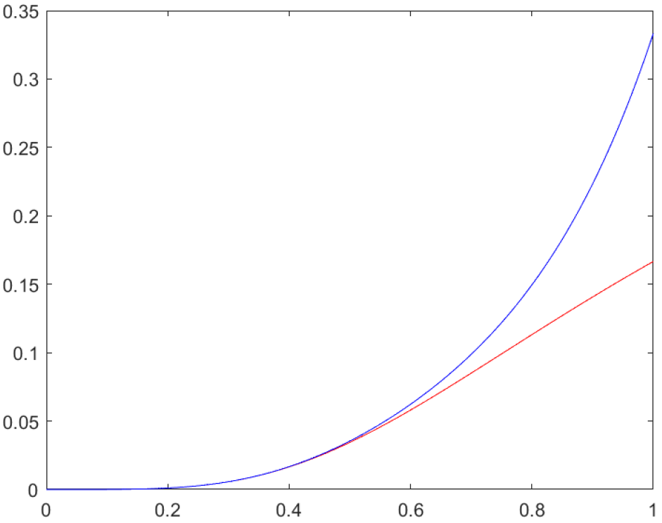
The validity of (5) can be observed in Figure 1. The red line in the graphic is the left member and the blue line in the graphic is the right member of (5) from Theorem 6.
3.2. Quantum Integral Inequalities for Convex Functions
This second result is the main result for the last theorem of this subsection, and is a refinement of the parametric identity given in Lemma 2 from [28] when we consider a second parameter m.
Lemma 2.
Let be a twice q-differentiable function on and , . Moreover, if the function, and are continuous and q-integrable over , then we have:
where
Proof.
The demonstration is similar to the proof of Lemma 1. We consider as the expression and is the expression , we have .
By using Definition 5 of the right quantum derivative of k, we will obtain
Utilizing Definition 7, of the right q-integral of k, and using calculus, we have,
From Definition 6 of the left quantum derivative of k, we have
Utilizing Definition 8, of the left quantum integral of k, and then using calculus, we get
Then, multiplying the expression by , it follows that
which completes the proof. □
Remark 2.
Lemma 1 from [28] is a consequence of Lemma 2 when the parameter .
Theorem 10.
Under conditions of Lemma 2, if and are convex functions on , then the following will be obtained
Proof.
The properties of the modulus with the convexity of and will help us to prove the following inequalities:
which completes the proof. □
Remark 3.
It could be given some similar applications to special means as arithmetic mean, harmonic mean, and geometric mean of real numbers by using the established results as in [26].
4. Discussion and Conclusions
The main findings of this work are intended to prove novel parametrized q-Hermite–Hadamard-like type integral inequalities for mappings whose third left and right q-derivative in absolute value have s-convex and -convex, respectively. The main inequalities, quantum Holder’s integral inequality and quantum power mean inequality, have been utilized to obtain the new estimated bounds. Two auxiliary quantum lemmas have been used as a basic tool in our proofs in the two subsections of Section 3. Several consequences appear for special choice of as a parameter in the first subsection of Section 3, and the corresponding example was analyzed and discussed in detail to illustrate the obtained results, in order to prove the consistency of the conclusions. The obtained results could be useful in certain optimization studies. Convex functions have applications in fields of applied sciences such as numerical analysis, approximation theory, optimization and statistics, which can be useful tools in economy and business.
We used the Matlab R2023a software version, as a tool, for the figure and for some calculus in the given example. The researchers can establish similar inequalities for coordinated convex functions in the future.
We hope that the results will continue to sharpen our understanding of the nature of q-calculus, and as a further study, it could be interesting to extend these findings to recent newly defined kinds of convexities, to -calculus, and to q-fractional calculus, which would be several good generalizations.
Author Contributions
Conceptualization, L.C. and E.G.; methodology, L.C.; software, L.C.; validation, L.C. and E.G.; formal analysis, L.C.; investigation, L.C. and E.G.; resources, L.C. and E.G.; data curation, L.C.; writing—original draft preparation, L.C.; writing—review and editing, L.C. and E.G.; visualization, L.C. and E.G.; supervision, L.C. and E.G.; project administration, L.C. and E.G.; funding acquisition, L.C. and E.G. All authors have read and agreed to the version of the manuscript.
Funding
This research received no external funding.
Data Availability Statement
Data is contained within the article.
Conflicts of Interest
The authors declare no conflicts of interest.
References
- Jackson, F.H. On q-functions and a certain difference operator. Trans. R. Soc. Edinb 1909, 2, 253–281. [Google Scholar] [CrossRef]
- Jackson, F.H. On q-definite integrals. Q. J. Pure Appl. Math. 1910, 41, 193–203. [Google Scholar]
- Ernst, T.A. Comprehensive Treatment of q-Calculus; Springer: Basel, Switzerland, 2012. [Google Scholar]
- Kac, V.; Cheung, P. Quantum Calculus; Springer: New York, NY, USA, 2003; p. 652. [Google Scholar]
- Tariboon, J.; Ntouyas, S.K. Quantum integral inequalities on finite interval. J. Inequal. Appl. 2014, 121, 13. [Google Scholar] [CrossRef]
- Tariboon, J.; Ntouyas, S.K. Quantum calculus on finite intervals and applications to impulsive difference equations. Adv. Differ. Equ. 2013, 282, 19. [Google Scholar] [CrossRef]
- Hadamard, J. Etude sur les proprietes des fonctions entieres en particulier d’une fonction consideree par Riemann. J. Math. Pures. Appl. 1893, 58, 171–215. [Google Scholar]
- Dragomir, S.S.; Pearce, C.E.M. Selected Topics on Hermite-Hadamard Inequalities and Applications; RGMIA Monographs, Victoria University: Melbourne, Australia, 2000. [Google Scholar]
- Alomari, M.; Darus, M. Co-ordinated s-convex function in the first sense with some Hadamard-type inequalities. Int. J. Contemp. Math. Sci. 2008, 3, 1557–1567. [Google Scholar]
- Dragomir, S.S. On Hadamard’s inequality for convex functions on the co-ordinates in a rectangle from the plane. Taiwanese J. Math. 2001, 5, 775–788. [Google Scholar] [CrossRef]
- Alomari, M.; Latif, M.A. On Hadamard-type inequalities for h-convex functions on the co-ordinates. Int. J. Math. Anal. 2009, 3, 1645–1656. [Google Scholar]
- Khan, A.; Chu, Y.M.; Khan, T.U.; Khan, J. Some inequalities of Hermite-Hadamard type for s-convex functions with applications. Open Math. 2017, 15, 1414–1430. [Google Scholar] [CrossRef]
- Alomari, M.; Darus, M.; Kirmaci, U.S. Some inequalities of Hermite-Hadamard type for s-convex functions. Acta Math. Sci. 2011, B, 1643–1652. [Google Scholar] [CrossRef]
- Barsam, H.; Ramezani, S.M.; Sayyari, Y. On the new Hermite-Hadamard type inequalities for s-convex functions. Afr. Math. 2021, 32, 1355–1367. [Google Scholar] [CrossRef]
- Kunt, M.; Iscan, I. Fractional Hermite-Hadamard-Fejer type inequalities for GA-convex functions. Turk. J. Inequal. 2018, 2, 1–20. [Google Scholar]
- Kalsoom, H.; Hussain, S. Some Hermite-Hadamard type integral inequalities whose n-times differentiable functions are s-logarithmically convex functions. Punjab Univ. J. Math. 2019, 51, 65–75. [Google Scholar]
- Ciurdariu, L. On some Hermite-Hadamard type inequalities for functions whose power of absolute value of derivatives are (α,m)-convex. Int. J. Math. Anal. 2012, 6, 2361–2383. [Google Scholar]
- Ciurdariu, L. Hermite-Hadamard type inequalities for fractional integrals operators. Appl. Math. Sci. 2017, 11, 1745–1754. [Google Scholar] [CrossRef]
- Khan, M.A.; Anwar, S.; Khalid, S.; Sayed, Z.M.M.M. Inequalities of the type Hermite-Hadamard-Jensen-Mercer for strong convexity. Math. Probl. Eng. 2021, 2021, 5386488. [Google Scholar]
- Xu, P.; Butt, S.I.; Ain, Q.U.I.; Budak, H. Nex estimates for Hermite-Hadamard inequality in quantum calculus via (α,m) convexity. Symmetry 2022, 14, 1394. [Google Scholar] [CrossRef]
- Alp, N.; Budak, H.; Sarikaya, M.Z.; Ali, M.A. On new refinements and generalizations of q-Hermite-Hadamard inequalities for convex functions. Rocky Mt. J. Math. 2023. Available online: https://projecteuclid.org/journals/rmjm/rocky-mountain-journalof-mathematics/DownloadAcceptedPapers/220708-Budak.pdf (accessed on 4 June 2023).
- Alp, N.; Sarikaya, M.Z.; Kunt, M.; Iscan, I. q2-Hermite-Hadamard inequalities and quantum estimates for midpoint type inequalities via convex and quasi-convex functions. J. King Saud Univ. Sci. 2018, 30, 193–203. [Google Scholar] [CrossRef]
- Jhanthanam, S.; Tariboon, J.; Ntouyas, S.K.; Nonlaopon, K. On q-Hermite-Hadamard inequalities for differentiable convex functions. Mathematics 2019, 7, 632. [Google Scholar] [CrossRef]
- Zhao, D.; Ali, M.A.; Luangboon, W.; Budak, H.; Nonlaopon, K. Some Generalizations of Different Types of Quantum Integral Inequalities for Differentiable Convex Functions with Applications. Fractal Fract. 2022, 6, 129. [Google Scholar] [CrossRef]
- Latif, M.A.; Kunt, M.; Dragomir, S.S.; Iscan, I. Post-quantum trapezoid type inequalities. AIMS Math. 2020, 5, 4011–4026. [Google Scholar] [CrossRef]
- Ciurdariu, L.; Grecu, E. Several quantum Hermite-Hadamard-type integral inequalities for convex functions. Fractal Fract. 2023, 7, 463. [Google Scholar] [CrossRef]
- Noor, M.; Noor, K.; Awan, M. Quantum Ostrowski inequalities for q-differentiable convex functions. J. Math. Inequal. 2016, 10, 1013–1018. [Google Scholar] [CrossRef]
- Ciurdariu, L.; Grecu, E. New perspectives of symmetry conferred by q-Hermite-Hadamard type integrals. Symmetry 2023, 15, 1514. [Google Scholar] [CrossRef]
- Orlicz, W. A note on modular spaces I. Bull. Acad. Polon. Sci. Math. Astronom. Phys. 1961, 9, 157–162. [Google Scholar]
- Hudzik, H.; Maligranda, L. Some remarks on s-convex functions. Aequationes Math. 1994, 48, 100–111. [Google Scholar] [CrossRef]
- Bermudo, S.; Korus, P.; Valdes, J.N. On q-Hermite-Hadamard inequalities for general convex functions. Acta Math. Hung. 2020, 162, 364–374. [Google Scholar] [CrossRef]
- Rajkovic, P.M.; Stankovic, M.S.; Marinkovic, S.D. The zeros of polynomials orthogonal with respect to q-integral on several intervals in the complex plane. In Proceedings of the Fifth International Conference of Geometry Integrability and Quantization, Varna, Bulgaria, 5–12 June 2003; pp. 178–188. [Google Scholar]
Figure 1.
Example for the inequality (6) from Theorem 6.

Disclaimer/Publisher’s Note: The statements, opinions and data contained in all publications are solely those of the individual author(s) and contributor(s) and not of MDPI and/or the editor(s). MDPI and/or the editor(s) disclaim responsibility for any injury to people or property resulting from any ideas, methods, instructions or products referred to in the content. |
© 2023 by the authors. Licensee MDPI, Basel, Switzerland. This article is an open access article distributed under the terms and conditions of the Creative Commons Attribution (CC BY) license (https://creativecommons.org/licenses/by/4.0/).
Share and Cite
MDPI and ACS Style
Ciurdariu, L.; Grecu, E. On q-Hermite–Hadamard Type Inequalities via s-Convexity and (α,m)-Convexity. Fractal Fract. 2024, 8, 12. https://0-doi-org.brum.beds.ac.uk/10.3390/fractalfract8010012
AMA Style
Ciurdariu L, Grecu E. On q-Hermite–Hadamard Type Inequalities via s-Convexity and (α,m)-Convexity. Fractal and Fractional. 2024; 8(1):12. https://0-doi-org.brum.beds.ac.uk/10.3390/fractalfract8010012
Chicago/Turabian StyleCiurdariu, Loredana, and Eugenia Grecu. 2024. "On q-Hermite–Hadamard Type Inequalities via s-Convexity and (α,m)-Convexity" Fractal and Fractional 8, no. 1: 12. https://0-doi-org.brum.beds.ac.uk/10.3390/fractalfract8010012