
SeeCucumbers: Using Deep Learning and Drone Imagery to Detect Sea Cucumbers on Coral Reef Flats


1
College of Science and Engineering, James Cook University Townsville, Bebegu Yumba Campus, 1 James Cook Drive Douglas, Townsville, QLD 4811, Australia
2
TropWATER, College of Science and Engineering, James Cook University Townsville, Bebegu Yumba Campus, 1 James Cook Drive Douglas, Townsville, QLD 4811, Australia
3
TropWATER, College of Science and Engineering, James Cook University Cairns, Nguma-bada Campus, 14-88 McGregor Road Smithfield, Cairns, QLD 4878, Australia
4
School of Engineering and Mathematics Science, La Trobe University, Melbourne, VIC 3086, Australia
*
Author to whom correspondence should be addressed.
Drones 2021, 5(2), 28; https://0-doi-org.brum.beds.ac.uk/10.3390/drones5020028
Submission received: 25 March 2021
/
Revised: 11 April 2021
/
Accepted: 13 April 2021
/
Published: 16 April 2021
Abstract
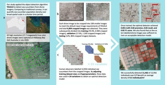
:Sea cucumbers (Holothuroidea or holothurians) are a valuable fishery and are also crucial nutrient recyclers, bioturbation agents, and hosts for many biotic associates. Their ecological impacts could be substantial given their high abundance in some reef locations and thus monitoring their populations and spatial distribution is of research interest. Traditional in situ surveys are laborious and only cover small areas but drones offer an opportunity to scale observations more broadly, especially if the holothurians can be automatically detected in drone imagery using deep learning algorithms. We adapted the object detection algorithm YOLOv3 to detect holothurians from drone imagery at Hideaway Bay, Queensland, Australia. We successfully detected 11,462 of 12,956 individuals over with an average density of 0.5 individual/m. We tested a range of hyperparameters to determine the optimal detector performance and achieved 0.855 mAP, 0.82 precision, 0.83 recall, and 0.82 F1 score. We found as few as ten labelled drone images was sufficient to train an acceptable detection model (0.799 mAP). Our results illustrate the potential of using small, affordable drones with direct implementation of open-source object detection models to survey holothurians and other shallow water sessile species.
1. Introduction
Sea cucumbers (Holothuroidea), or holothurians (also known as bêche de mer), are a valuable fishery resource due to their high market demand [1,2,3,4]. They also play an important role as recyclers of nutrients to other trophic levels, hosts for many biotic associates, and crucial bioturbation agents to maintain and improve the sediment quality [5,6]. Species such as Holothuria atra, H. mexicana, Isostichopus badionotus, and Stichopus chloronotus are prolific bioturbators, capable of processing the upper 3 to 5 mm of all marine sediments available in their habitat at least once per annum [6,7]. Since the volume of sediments ingested and defecated by sea cucumber is remarkable (9–82 kg per individual per year), their role in maintaining biodiversity, primary productivity, and sediment health could be substantial over long timescales in areas where they are highly abundant [5]. For example, a recent study calculated that Holothuria atra were likely responsible for the bioturbation of more than 64,000 metric tonnes per year at Heron Island Reef in the southern Great Barrier Reef [8]. Therefore, investigating the population dynamics and distribution patterns of common holothurian species are important steps to quantify their fishery value and their ecological functions in the ecosystem.
Past population and movement pattern surveys have established that holothurians are unevenly distributed in reef systems [9,10] and able to travel a distance from 1 m to 9 m daily [7,11,12]. These patterns are usually documented using conventional in situ survey methods plotting the movement pattern of a small number of individuals (ranging from 10 to 100) over 24 h [7,11,12]; or by counting holothurians along transect lines or quadrats by walking [13], snorkelling [14], SCUBA diving [11] or during manta tows [9,15]. Although these traditional direct visual census approaches enable estimation of the density or quantification of the likely ecological functions of holothurians, they can be labour intensive, expensive, prone to errors, non-replicable, and biased due to observer expertise [16,17]. Additionally, the results are obtained through extrapolation from small spatial footprints, short sampling times, and long temporal intervals [6,18], which may not account for the broader spatial or longer temporal scale variations of holothurian studies. Consequently, there is a need to develop more effective and efficient tools to monitor sea cucumbers and similar marine invertebrates over broader scales.
Advances in electronic, optical, and computational technology, using remote sensing (RS) techniques with machine learning (ML) algorithms offers a potential solution to monitor holothurians and other sessile marine species over broad scales. RS offers a quick and synoptic overview of ecological features as well as providing repeatable, standardised, and verifiable information on long-term trends in ecosystem structure and processes [19,20]. Currently, RS is applied in various marine environments at different scales, including, but not limited to, marine vertebrate surveys, shoreline monitoring, coral bleaching events trajectory, coral reef bathymetry mapping, and marine habitat classification [21,22,23,24,25,26,27,28]. However, RS techniques rely on tremendous amounts of data, which would exceed conventional human power for direct visual inspection [29]. Human errors and fatigue can introduce inconsistencies while researchers are trying to draw conclusions. This has driven the use of ML models with computer vision to automatically recognise and identify specific targets of interest. Furthermore, deep learning (DL), a subfield of ML, has become increasingly popular since 2006 [30]. Convolutional neural networks (CNN) are considered to be the most representative DL model and a more powerful tool for object detection compared to traditional ML frameworks [30]. While RS techniques have become more affordable, many new and robust CNN architectures have also been developed open source and made readily available for researchers. These advances warrant further investigation of RS and DL based object detection of marine invertebrates (like sea cucumbers) for broad scale identification and density estimation.
Since the typical length of a mature holothurian individual is between 20 and 40 cm [31], the required spatial resolution for successful identification is at most 2–4 cm. Hence, unoccupied aerial vehicles (UAV, i.e., drones), rather than satellites, are a suitable platform to capture data appropriate for sea cucumber detection. A consumer-level drone can easily achieve a ground sampling distance (GSD) of 2 cm at 100 m altitude with a digital camera [32]. In addition, many CNN object detection algorithms such as You Only Look Once (YOLO) [33,34] are now easily accessible by researchers via open source deep learning computing tools like TensorFlow [35], Pytorch [36], and Keras [37]. Yet so far, only one study has used a CNN architecture (ResNet50) to detect holothurians from drone imagery for the purpose of population estimation in natural habitat [16]. They compared three methods: counting sea cucumbers using an ML algorithm from drone imagery, manual counting from drone imagery, and in situ counting along transects by snorkellers [16]. The study found that using an ML algorithm and performing manual counting by observers were similar to the counts obtained from in water transects at a relatively low density, but began to underestimate when the density surpassed 75 sea cucumbers per 40 m (i.e., 1.88 individuals/m) [16]. They also pointed out that the time required to extract manual counts from drone images was higher than in-water surveys [16]. The potential of an efficient automatic holothurian detection process would reduce the time and labour requirements significantly over broad spatial scale. However, improving the efficiency of a detection model remains a knowledge gap worthy of further investigation.
The efficiency of a detection model could be improved by using more advanced hardware, faster DL algorithms, or better training procedures. More powerful hardware could shorten the computing time for both training and detection, but such improvement is beyond the control of ecologists. Training regimes and DL algorithms, on the other hand, can be implemented and optimised by any developer or researcher with programming ability, such as by changing the input training dataset, tuning the hyperparameters of learning algorithms, selecting different evaluation metrics, etc. The size of the training dataset determines the time and labour required to prepare the data (i.e., labelling holothurians in our case). Hyperparameters are the configurations of the learning algorithm itself before the learning process starts (i.e., the selection of pre-trained weights and anchor boxes, see Section 2.3.3) which impacts the performance of the resulting model [38]. In this study, we selected the third version of YOLO (YOLOv3) due to its widespread use in the literature and industry and well established open source community of support. It also offers faster processing with minimal reduction in performance when compared to other object detection models, such as Single-Shot Detector, RetinaNet, and Regions with CNN (R-CNN) [34].
Our work contributes an automatic holothurian detection model using the YOLOv3 architecture and was delivered through the following steps: (1) summarized common evaluation metrics to select the most suitable for assessing holothurian detection models; (2) investigated the minimum training and labelling dataset sizes required to achieve an acceptable detection model; (3) tuned the YOLOv3 hyperparameters to select the optimal detection model; and (4) applied the optimal training model to quantify the density of holothurians at Hideaway Bay reef in North Queensland, Australia.
2. Methods
2.1. Study Site
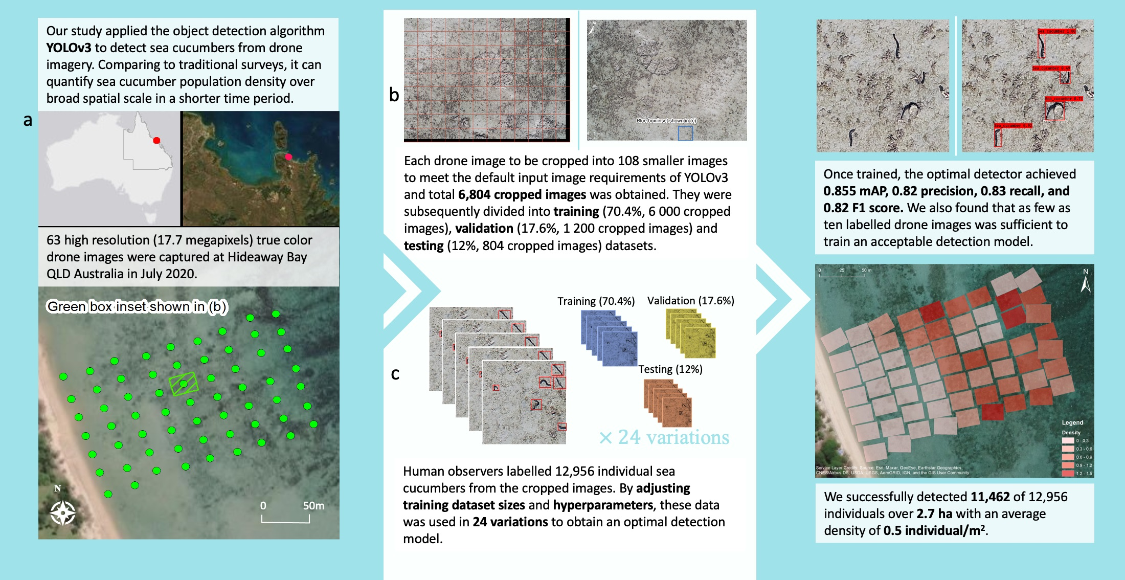
Hideaway Bay (20.072 914° S 148.481 359° E) is a mainland attached fringing reef located on Cape Gloucester in the Mackay Whitsunday Region of North Queensland, Australia (Figure 1a). The reef extends up to 350 m offshore and over 3 km alongshore [39]. A recent survey showed that the environmental conditions at monitoring sites in this region are generally characterised by relatively high turbidity and high rates of sedimentation [40] with the reef flat largely dominated by terrigenous sediments [39]. Little information about holothurian population is known in this area. Yet easy access and calm weather made it an ideal site for drone imagery data collection.
2.2. Data Acquisition
Drone imagery was captured in July 2020 using a DJI Phantom 4 Pro—a multirotor drone suitable for flying slowly at low altitudes and taking off and landing in small spaces. We used the free Drone Deploy mission planning app to create a flight path over the area of interest at 20 m altitude with 75% overlap and 75% sidelap between nadir images, suitable for creating an orthomosaic in future studies. As the orthomosaic process can introduce errors such as double mapping or ghosting when combining overlapping images [41], we considered individual images better suited to our counting sea cucumber application. We therefore selected 63 of the total images, representing only those with no or very little overlap (every fourth photo along a run, and every fourth flightline). The resolution of these images was 4864 × 3648 pixels (px) (FOV = 73.7, GSD = 0.57 cm) (Figure 1b). The average area of one drone image was approximately 423 m (Figure 1b). Since the clarity of marine based drone imagery is subject to turbidity, wave conditions, and light and shade variation, all images were taken at low tide under calm conditions with a low level of turbidity [42] to minimize the training dataset complexity. Generally speaking, taking images in the early morning can minimize the sun glint and a wind speed less than 5 knots will not create significant ripples or waves that reduce the image quality [42]. A total area of 26,662 m (∼2.7 ha) was surveyed.
2.3. Data Processing
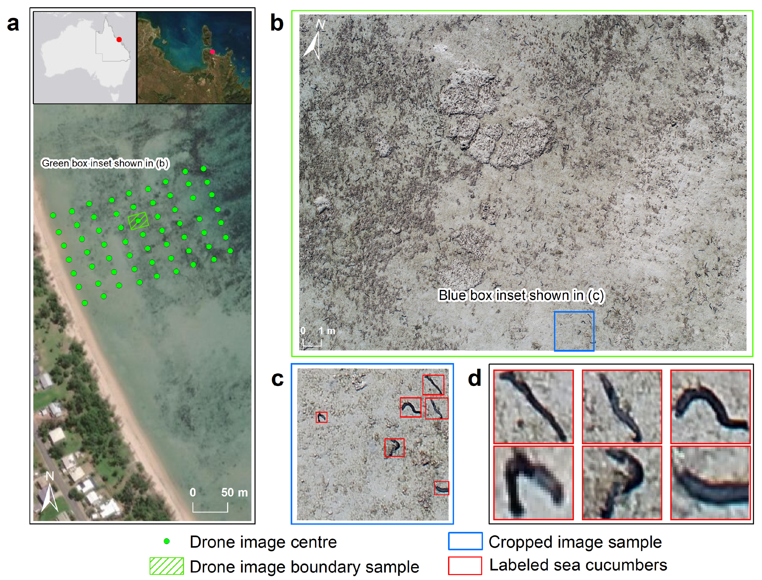
Data were processed through five major steps (Figure 2): (a) pre-process drone images; (b) use bounding boxes to label holothurians as required by YOLOv3 and prepare different sized training datasets to investigate the influences of dataset size on training results; (c) train and validate models using YOLOv3 deep learning object detection algorithm by tuning zero, one or two hyperparameters (for details see Section 2.3.3); (d) evaluate and determine an optimal holothurian detection model using common object evaluation metrics; and (e) apply the optimal detection model to map the sea cucumber density in the area of interest.
2.3.1. Image Pre-Processing
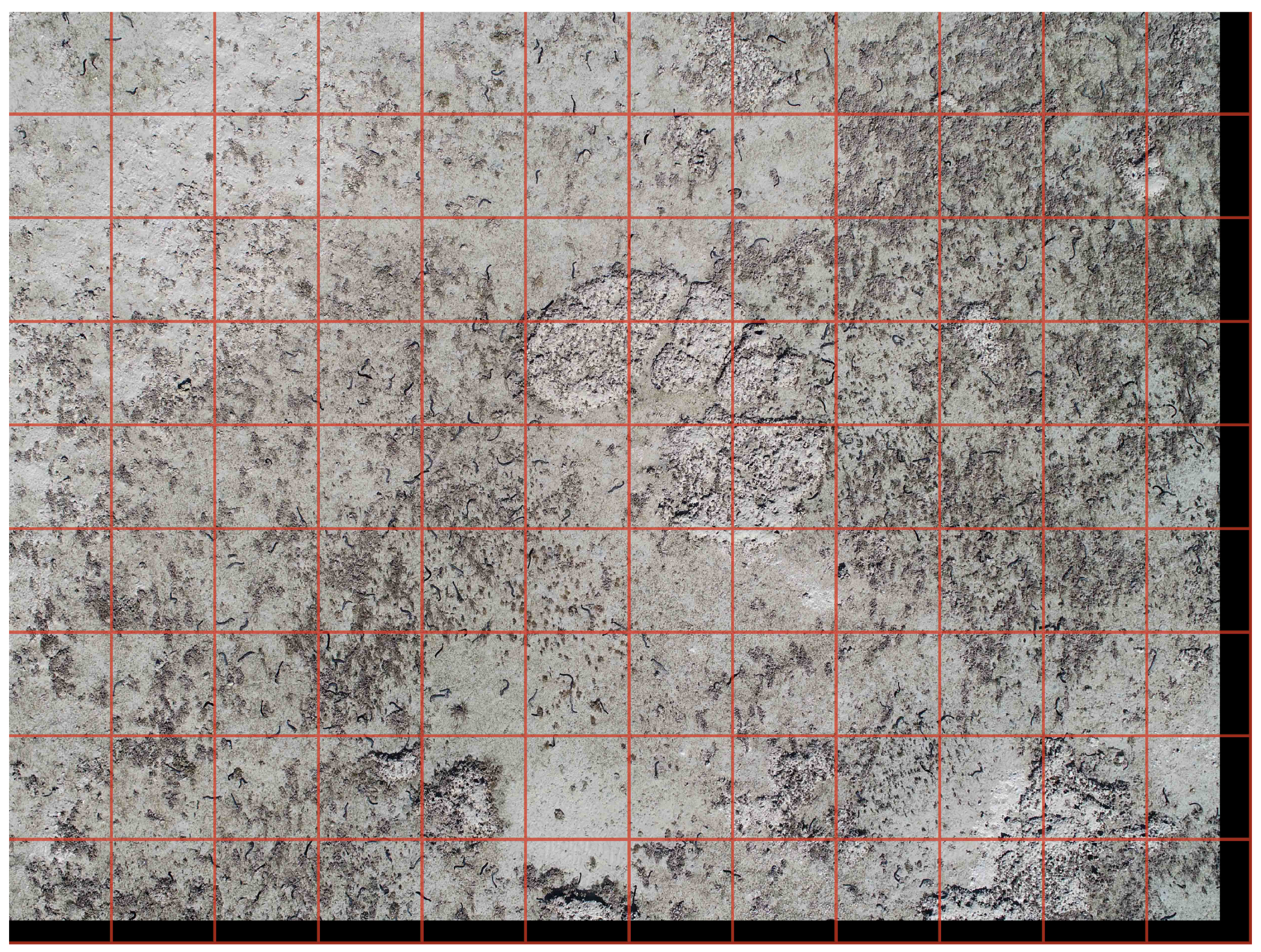
The 63 drone images were cropped to the default image input size of YOLOv3, 416 × 416 px (Figure 1c). As shown in Figure 3, each drone image is cropped into 108 smaller images (9 rows and 12 columns) giving a total 6804 cropped images was obtained. The cropped images at the last row and column were resized (i.e., padded with black pixels, see Figure 3) in order to meet the default settings of YOLOv3 input images. This resizing approach allows images to preserve the aspect ratio and provide positive sea cucumber information without affecting the classification accuracy [43].
2.3.2. Labelling and Dataset Preparation
Each cropped image was manually examined and each sea cucumber was identified and labelled manually by three trained volunteers using Labelme [44]. In order to maximize the available useful information, sea cucumbers under all conditions (fully exposed on sandy bottom or on coral reefs, partially covered by sediments or rubbles, cutoff by the edges of the images, etc.) were labelled with a tight rectangular box (Figure 1c,d). The pixel coordinates of the top left and bottom right corner of each box were saved with annotations in a JSON file for each cropped image, which was used as ground truth for later analyses. The cropped and labelled images were first randomly split into two subsets: training and validation (88%) and testing (12%). The testing dataset comprised 804 images that were reserved for ultimate model evaluation, which was never used during the training and validation. The ML training and validation dataset comprised 6000 images. To study the importance of training sample size and identify the optimal number of labelled images required this subset was randomly sampled into six training sets composed of 1000, 2000, 3000, 4000, 5000, and 6000 images. Each of the six training datasets were further split into 80% training (800, 1600, 2400, 3200, 4000, and 4800 cropped images, respectively) and 20% validation (200, 400, 600, 800, and 1200 cropped images, respectively) to facilitate the deep learning training process.
2.3.3. Model Training and Validation
YOLOv3 is an open-source deep learning object detection algorithm with CNN architecture (Darknet50) [34] that is often trained with hyperparameter tuning tailored for specific applications. For the purpose of this study we used a high performance computer to implement YOLOv3 [45] with Python 3.6, Keras 2.2.4 [37], and TensorFlow 1.13 [35]. We tuned two hyperparameters before starting the learning process: pre-trained model weights and anchor box size. By definition, pre-trained model weights are used during transfer learning, which refers to the situation of learning in a new setting through the transfer of knowledge from a related setting that has already been learned [46]. Meanwhile, anchor boxes serve as the initial guesses of the bounding boxes for detected objects [47]. Faster progress or improved performance are often expected by adopting such variations. The default settings for these two hyperparameters in YOLOv3 are using anchor boxes and pre-trained model weights obtained from the COCO dataset [45]. In this study, four modifications of hyperparameters were adopted as follows:
- Scenario A: zero hyperparameters tuned: default pre-trained model weights and default anchor boxes.
- Scenario B: one hyperparameter tuned: default pre-trained model weights and modified anchor boxes.
- Scenario C: one hyperparameter tuned: modified pre-trained model weights and default anchor boxes.
- Scenario D: two hyperparameters tuned: modified pre-trained model weights and modified anchor boxes.
To modify the anchor boxes, we changed their size and shape using k-means clustering of the labelled bounding boxes in sea cucumber dataset (scenarios B and D above) [34]. To determine the influence of the pre-trained model weights, the COCO derived pre-trained model weights were changed to random numbers (scenarios C and D above). Combining the four hyperparameter tuning scenarios (A–D above) and the six different sized training datasets (i.e., 1000–6000), there were 24 training variations.
2.3.4. Sea Cucumber Detection Evaluation
The detection models were applied to the ultimate unseen testing dataset (804 images) that had not been used in any of the previous training scenarios. Here we used the evaluation metrics adapted from commonly used evaluation metrics in Keras and TensorFlow libraries [48], the 2020 COCO Object Detection challenge [49,50] and the PASCAL VOC Challenge [51]. These include intersection over union (IOU), mean average precision (mAP), precision, recall, and F1 scores, which are calculated based on confusion matrices and confidence scores. A confusion matrix is the combination of ground truth data and detected results from an ML model, whereas the confidence score is a value measured by a detection model showing the certainty of the results (from 0 to 1, i.e., from not confident to very confident) [48]. The object detection evaluation metrics were calculated and interpreted as described in Table 1.
The evaluation metrics measure the effectiveness of the model, and are thus influential in determining model selection according to the users’ requirements [48]. For instance, choosing a model with maximum F1 or mAP score would be the best option if the goal is to achieve a good balance between precision and recall. In other cases, high precision would be preferred if the desired information is about the exact location of sea cucumbers, whereas high recall would be preferred if more accurate population counting is needed. To achieve either higher precision or higher recall, the model’s training and detection result can be adjusted by modifying the IOU (intersection over union) and confidence score threshold. In this study, the goal was to produce a density map of sea cucumbers, and both precision and recall values were important. Thus, using the F1 score or mAP which combines precision and recall scores was preferred. In this work, one object class was designated to group all sea cucumber species. In future, multiclass object detection within image for other taxa or specific sea cucumber species could be investigated by adding separate object classes for each target of detection. Thus, the mAP was chosen as the primary criteria since it allows for the addition of more object classes in the future. Since there has been no research recommending an absolute mAP value to determine whether the performance of a model is acceptable, we used the top result in COCO Detection Leaderboard (mAP = 0.770) as the judging criteria [52].
2.3.5. Mapping Sea Cucumber Density
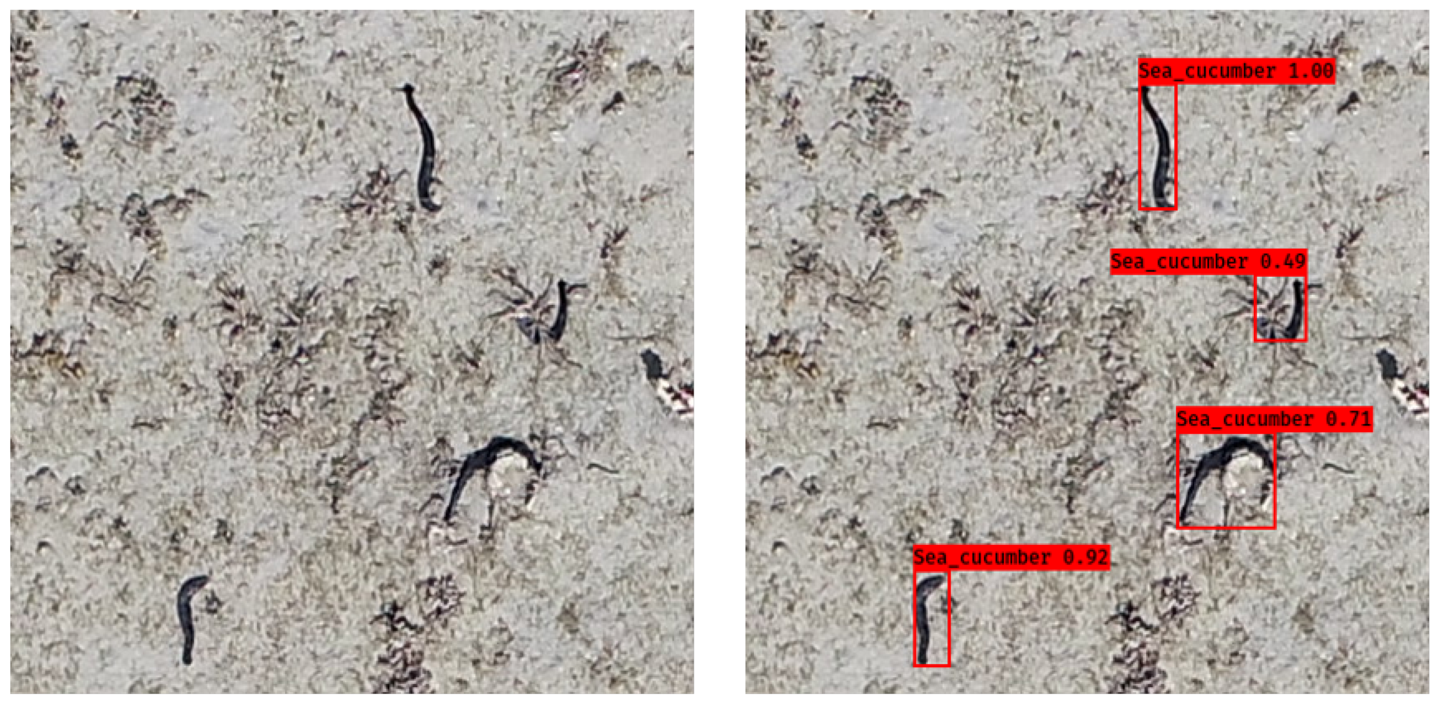
The output of the detection model was superimposed onto the input image detailing the location and confidence score of the output prediction within the image (Figure 4). The detected results of sea cucumber counts in each cropped image were added together to calculate the number of sea cucumbers present in the complete drone image using the optimal model obtained above. The images were georeferenced according to the geotagged metadata of the drone images and visualised as a sea cucumber density (i.e., number of sea cucumbers/area of the drone image) footprint map in ArcGIS Desktop 10.7 [53].

Table 1.
Criteria commonly used to assess and evaluate the performance of machine learning models [48,51,54].
| Evaluation Metrics | Definitions | Interpretation and Relevance | |||
|---|---|---|---|---|---|
| Intersection over Union (IOU) |  | By using an IOU threshold of 0.5 to define true positive detections we required that at least 50% of the bounding box area identified by the ML approach overlapped with the area identified by the human observer. A higher IOU threshold would indicate a higher accuracy of the detection location within an image, and thus result in less true positive detections. In this study, a moderate IOU threshold (0.5) was chosen to compare with other object detection challenges (used for both COCO and PASCAL VOC object detection challenge) [49,51] and as the exact location of a sea cucumber individual was not the priority. | |||
| where A is the area of the detected bounding box and B is the area of the mannually labelled bounding box. | |||||
| Confusion/ Error matrix | Predicted by ML model | A bounding box is deemed a TP, TN, FN, or FP when the confidence score (in this case it was set to 0 to evaluate the performance) and IOU exceed the chosen threshold (in this case IOU ≥ 0.5). The numbers of the TP, TN, FN, and FP detected results alone do not indicate the performance quality of resulting model but are the basic values used to calculate other evaluation metrics. | |||
| Positive | Negative | ||||
| Ground Truth | Positive | True Positive (TP) | False Negative (FN) | ||
| Negative | False Positive (FP) | True Negative (TN) | |||
| Precision | Precision values range from 0 for very low precision to 1 for perfect precision. Higher precision means higher correct detection in all detected results, i.e., more detected sea cucumbers are actually sea cucumbers. High Precision value was preferred if the detected sea cucumber correctly in this study. | ||||
| where TP is the number of true positives and FP is the number of false positive detected results. | |||||
| Recall | Recall values range from 0 for poor recall to 1 for perfect recall. Higher recall means less incorrect detections, i.e., less detection of objects that are not sea cucumbers. | ||||
| where TP is the number of true positive and FN is the number of false negative detected results. | |||||
| F1 score | This is the harmonic mean of precision and recall. The closer the F1 score is to a value of 1 the better the performance of the model. Instead of choosing either the model with the best precision or the best recall, the highest F1 score balances the two values. It is useful when both high precision and high recall are desired. | ||||
| mAP | This metric is similar to the F1 score, but with the benefit that it has the potential to measure multiple categories if required. | ||||
| where N is the number object classes being detected (in our case, N = 1 since we only detect se cucumbers), n is the number of recall levels (in an ascending order) at which the precision is first interpolated, r is recall, and p is precision [51,54]. | |||||
3. Results and Discussion
A total of 6804 cropped images were created and a total of 12,956 sea cucumbers were manually labelled. Based on the evaluation, the performance of the detection models were influenced by size of the training dataset and the hyperparameters used as described and discussed below.
3.1. Model Performance Evaluation
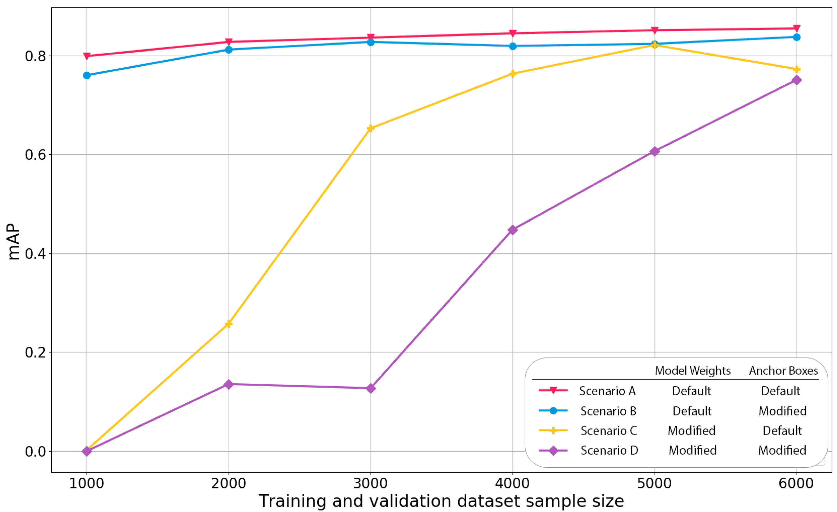
Of the 24 variations tried the worst performance was training with modifying both hyperparameters (Scenario D) and using the smallest training dataset (1000), which was unable to detect any sea cucumbers resulting in an mAP value of 0 (Figure 5). The best detection result (mAP = 0.855) was achieved using 6000 cropped training images with no changes in default hyperparameters (Scenario A). The relevant optimal confidence score threshold was found to be 0.27, which resulted in 0.82 precision, 0.83 recall, and 0.82 F1 score, respectively, (Table 2). This indicates that 82% of sea cucumbers detected were correct and more than 83% of true sea cucumbers were detected. The details of mAP variation and the associated precision and recall curves are provided in the Appendix A Table A1.
3.1.1. Influence of Training Dataset Size
Without considering the impacts of hyperparameter tuning, the increasing training data sample sizes improved the model performance (Figure 5 and Table 2). In scenarios A and B, the mAP value improved very marginally as the training dataset size increased from 1000 images (Scenario A = 0.799, Scenario B = 0.760) to 6000 images (Scenario A = 0.855, Scenario B = 0.838) (i.e., from 10 to 56 uncropped drone images). Yet in scenarios C and D, where the pre-trained model weights were removed, the mAP value increases dramatically as the training dataset size increased (Scenario C from 0.002 to 0.773, Scenario D 0.000 to 0.750). Moreover, the training dataset size was also the major factor determining the training time needed. Each 1000 images contributed approximately one hour worth of training time. If using the best mAP for COCO dataset as the judging criteria (i.e., mAP = 0.770) [52], the minimum dataset size required to train an acceptable sea cucumber detection system would be 1000 cropped images (i.e., less than 10 drone images) under Scenario A (mAP = 0.799 > 0.770). This number, however, may be subject to change due to various conditions including more diverse sea cucumber species presented, higher turbidity in the water column or worse weather condition.
3.1.2. Influence of Hyperparameter Tuning
Hyperparameter tuning had negative impacts on the detection models, which was different from our original expectation. The average mAP, including all training dataset sizes, with no tuning of the default hyperparameters (Scenario A) was 0.835 (Table 2). An average mAP of 0.813 was achieved by changing the anchor box size (Scenario B) and an average mAP of 0.545 was achieved by removing the COCO derived pre-trained model weights (Scenario C). Changing both hyperparameters (Scenario D) resulted in the lowest average mAP (0.345). Using the default pre-trained model weights means the model has been optimized by exposure to more than 120,000 labelled images [34,49] before the specific sea cucumber training, which made it better at recognizing patterns, colours, textures, etc. Without it, the basic feature recognition was learnt from scratch only from the labelled sea cucumber images. Therefore, providing more images during the training significantly improved the output (Figure 4 scenarios C and D).
Using default anchor boxes also performed better than using modified anchor boxes, which agrees with the original YOLOv3 paper which stated that while changing anchor boxes might improve the performance of the model, it could decrease the model stability [34]. Hence, keeping the default hyperparameters of YOLOv3 was preferrable for our dataset. However, it is still questionable whether using pre-trained model weights will always improve the model performance. If the dataset being studied is sufficiently diverse and large, training from scratch could outperform training from pre-trained weights derived from common object datasets.
3.1.3. Comparison to Previous Studies
It is also important to compare the performance between different DL algorithms rather than just focus on YOLOv3 alone. The optimal detection values (IOU = 0.5, confidence score threshold = 0.27, precision = 0.82, recall = 0.83, mAP = 0.855, F1 = 0.82) compare favourably with past ecological studies that utilise machine learning. Kilfoil et al. [16] used a ResNet 50 CNN model to detect sea cucumbers from drone imagery in French Polynesia. They reported a similar evaluation metrics reporting various values (F1 score = 0.68, precision = 0.80, recall = 0.59) at a Minimum Validation Criteria (MVC) threshold of 0.25 [16]. In their study, the MVC is defined as “the minimum acceptable probability that an object is a sea cucumber for it to be counted as such” [16] (the equivalent concept to our confidence score threshold, which achieved 0.27 for the optimal model). The precision and recall in this study also exceeded the aforementioned citation [16], which was expected since YOLOv3 utilises different object detectors (faster RCNN vs. YOLOv3) and CNN backbones (ResNet 50 vs. Darknet 53) that should result in better and faster detection results [33,34]. However, such comparison across different studies are difficult since these studies often used different evaluation metrics and assess their models with different confidence thresholds. For instance, Beijbom et al. [55] uses Cohen’s kappa to evaluate the annotation accuracy of algae and hard corals, which varies from 43% to 96%. Villon et al. [56] reported fish species detection underwater have been shown to reach a bounding box overlap precision above 55% by using IOU = 0.5, T = 98%, where T was defined as a probability threshold. It is impossible to conclude that YOLOv3 is a better detector than faster RCNN or other algorithms. The differences could be a consequence of changing IOU threshold and using different training datasets with different image capture quality, water column variation, weather condition. Other environmental characteristics such as the complexity of the benthic habitat structure, the presence of holothurian-like organisms and coral reef patterns may also hinder or improve the performance of the object detection model. Since reproducibility is a major principle of scientific research, the failure to detail methodology and evaluation metrics in some ecological studies that utilise modern DL approaches becomes a shortcoming. The knowledge gap could be filled in the future by using the same datasets to compare the different CNN models and methodologies. This type of comparison requires researchers to make their datasets openly available to the community. The dataset and source code underlying this paper is made publicly available on GitHub (https://github.com/joanlyq/SeeCucumbers, accessed on 24 March 2021) and GeoNadir (https://data.geonadir.com/project-details/172, accessed on 24 March 2021) for future comparison.
3.2. Mapping Sea Cucumber Density
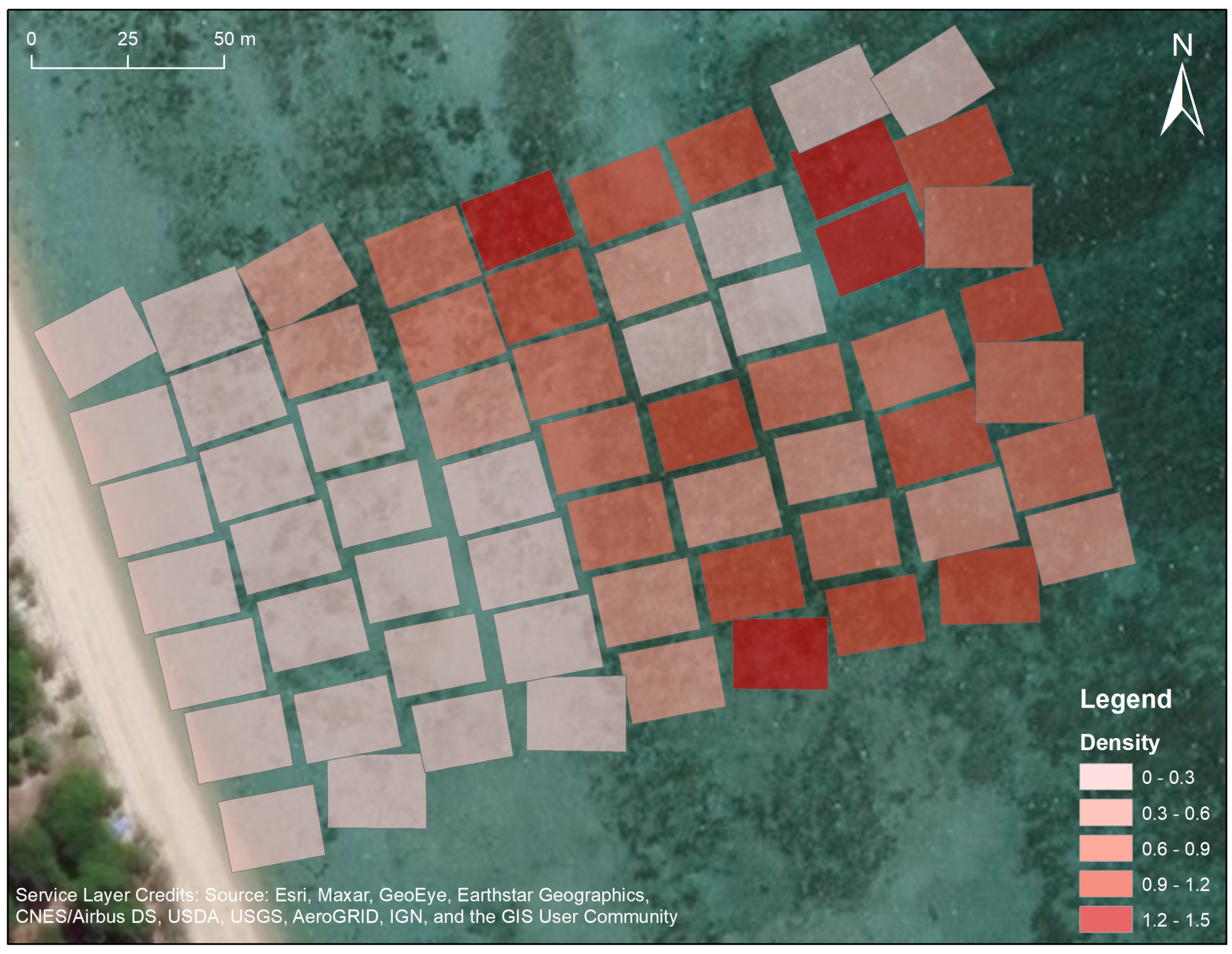
Within the area of each drone image, the maximum sea cucumber density ranged from 0 to 1.43 individuals/m (Figure 6) with an average density of sea cucumbers across the whole surveyed was area of 0.50 individuals/m. Details of sea cucumber density can be found in Table A2. A recent study at Heron Reef in the southern Great Barrier Reef used manually digitised drone images to calculate sea cucumber densities of 0.2 m on the shore adjacent sand dominated inner reef flat and 0.14 individuals/m2 at the coral dominated outer reef [8]. While those densities are comparable with our study, it is interesting to note that at Hideaway Bay higher densities of sea cucumbers tended to be found further from shore in areas of higher coral cover (Figure 6). Heron Reef has no terrestrial sediment inputs whereas Hideaway Bay has a mixed terrigenous and carbonate sediment environment [57]. However, further research and monitoring of sea cucumber populations at these two and other sites, is required to understand these trends.
3.3. Potential Future Applications
This implementation has demonstrated the potential of using state-of-the-art object detection algorithms with drone RS to quantify holothurian density in shallow reef environments. This method offers many benefits over current techniques by increasing efficiencies in both data capture and information extraction. Traditional survey methods only cover several hundred square meters in a day and track tens of individual sea cucumbers [6,7], whereas the drone images in this study collected data over an area size of in less than 30 min. The total dataset collection, labelling and training process in this work took approximately 48 h for the best model, and only eight hours for the minimum acceptable model (using less than ten drone images to train with default YOLOv3 hyperparameters that achieved a 0.799 mAP). Similar to previous studies, manually counting and labelling holothurians from drone images was the most time consuming element in the working process [8]. Using open source DL object detection models could provide a solution to reduce the counting time required for repeat surveys under similar water and other environmental conditions as the labelling and training process only needs to be done once. It detects and quantifies the counts of holothurians over broad spatial scale instead of extrapolating from small scale transects. Even if the detection model may require update as the dataset grows, it is usually a small proportion of the full dataset. The model can improve over time with better and larger training datasets across different locations. It also increases the reproducibility of studies and allows data to be reviewed and reanalysed by different experts.
Beyond these immediate improvements in workflows, automated sea cucumber detection from drone images is the first step toward further fruitful outcomes. It will allow researchers an entirely new stream of data regarding object level reef monitoring from aerial images. The detection model can be further applied to other ecological studies focusing on sessile marine invertebrates such as movement patterns, bioturbation contribution quantification, population dynamics, preferred habitats etc. Being able to detect the coordinates for target objects in geo-tagged drone images would allow the development of a faster and more automated locating process for distribution analysis. The density footprint map can be further combined with benthic habitat or bathymetry maps to gain more insights about the factors that impacting the distribution of sea cucumbers.
However, the current model is unable to detect holothurians to a species level. Thus, in situ surveys conducted by divers or snorkellers are complimentary with RS surveys and crucial to understand the ecological or biological function of specific species. Better understanding of holothurian physical and physiological characteristics of different species could help to overcome current shortcomings. Future improvements in the algorithm or the image data platform may also eliminate the negative influence of noise due to water column characteristics and accommodate environments that are more diverse. This means that methods and findings contained herein can also be used beyond the realm of the humble sea cucumber, and applied to many other benthic features. Finally, the faster and easier acquisition of data will allow for long term monitoring on a larger scale, which will improve the accuracy and efficiency of conservation management.
4. Conclusions
As people are becoming more aware of the ecological importance of sea cucumbers as well as their economic value, researchers are trying to devise efficient holothurian monitoring methods. There is also an increasing trend towards applying state-of-the-art machine learning technology to ecological studies. Our study not only presented an automatic sea cucumber detection model using drone imagery on coral reef flats, but also was the first one to apply the DL model to quantify the holothurian population and density over a broad spatial area. Under this workflow, we processed 63 high spatial resolution drone images of Hideaway Bay, Australia, and used YOLOv3 to detect holothurians. Performance was evaluated using common object detection metrics. All data and algorithms are open access and readily available online. In total, 11,462 out of 12,956 individuals were successfully detected, which were unevenly distributed across a area. The object detector performed well, achieving an mAP of 0.855, a precision of 0.82, a recall of 0.83 and an F1 score of 0.82. We found that as few as ten labelled drone images were sufficient to train an acceptable detection model (0.799 mAP). Collectively, these results illustrate the potential of using affordable unoccupied aerial vehicles (UAV, or drones) to survey and monitor holothurians and other shallow water sessile species with direct implementation of open source object detection models to increase the efficiency, replicability, and area able to be covered.
Author Contributions
Conceptualization, J.Y.Q.L., S.D., K.E.J. and W.X.; methodology, J.Y.Q.L. and W.X.; data collection: S.D.; formal analysis, J.Y.Q.L.; original draft preparation, J.Y.Q.L.; review and editing, S.D., K.E.J. and W.X. All authors have read and agreed to the published version of the manuscript.
Funding
This research received no external funding.
Institutional Review Board Statement
Not applicable.
Informed Consent Statement
Not applicable.
Data Availability Statement
Publicly available datasets were analyzed in this study. These data can be found here: https://github.com/joanlyq/SeeCucumbers, accessed on 24 March 2021, and https://data.geonadir.com/project-details/172, accessed on 24 March 2021.
Acknowledgments
We would like to thank Todd McNeill for their help in collecting drone imagery; Jane Williamson, Jordan Dennis, Edward Gladigau, Holly Muecke for their help in labelling the dataset. We owe deep gratitude to Jonathan Kok, Alex Olsen, Nicolas Younes, Redbird Furgeson, Raf Rashid for their valuable feedbacks of the manuscripts. We acknowledge useful assessments and correction from four anonymous reviewers as well as the journal editors.
Conflicts of Interest
The authors declare no conflict of interest.
Abbreviations
The following abbreviations are used in this manuscript:
| COCO | Common Object in Context dataset |
| CNN | Convolutional Neural Networks |
| DL | Deep Learning |
| FN | False Negative |
| FOV | Field of View |
| FP | False Positive |
| GSD | Ground Sampling Distance |
| IOU | Intersection Over Union |
| mAP | mean Average Precision |
| ML | Machine Learning |
| R-CNN | Regions with CNN |
| RS | Remote Sensing |
| TP | True Positive |
| TN | True Negative |
| UAV | Unoccupied Aerial Vehicles |
| YOLOv3 | You Only Look Once version 3 |
Appendix A
These are supplementary information for training and detection result.
Table A1.
Precision and recall curves summary of all 24 variations. The blue shaded area is equal to mAP of each variation and the red dot it the precision and recall level obtained from optimal confidence score threshold.
Table A1.
Precision and recall curves summary of all 24 variations. The blue shaded area is equal to mAP of each variation and the red dot it the precision and recall level obtained from optimal confidence score threshold.
| Training Dataset Size | Scenario | |||
|---|---|---|---|---|
| A | B | C | D | |
| 1000 |  |  |  |  |
| 2000 |  |  |  |  |
| 3000 |  |  |  |  |
| 4000 |  |  |  |  |
| 5000 |  |  |  |  |
| 6000 |  |  |  |  |
Table A2.
Drone image area size and the detected counts and density in each drone image as well as the ground truth and TP result from labelling.
Table A2.
Drone image area size and the detected counts and density in each drone image as well as the ground truth and TP result from labelling.
| Number | File Name | Image Area Size (m) | Detected Density (ind/m) | Detected Counts | Ground Truth | TP |
|---|---|---|---|---|---|---|
| 1 | DJI_0001 | 441.9 | 0.72 | 319 | 319 | 285 |
| 2 | DJI_0005 | 416.06 | 0.62 | 257 | 257 | 234 |
| 3 | DJI_0009 | 410.56 | 0.67 | 276 | 288 | 245 |
| 4 | DJI_0013 | 419.05 | 0.56 | 236 | 250 | 208 |
| 5 | DJI_0017 | 409.59 | 0.53 | 217 | 230 | 197 |
| 6 | DJI_0073 | 402.93 | 1.24 | 499 | 498 | 463 |
| 7 | DJI_0077 | 402.98 | 0.96 | 385 | 399 | 347 |
| 8 | DJI_0081 | 410.16 | 0.5 | 205 | 207 | 183 |
| 9 | DJI_0085 | 401.98 | 1 | 403 | 403 | 379 |
| 10 | DJI_0089 | 397.71 | 0.24 | 97 | 105 | 91 |
| 11 | DJI_0093 | 410.25 | 0.37 | 151 | 157 | 133 |
| 12 | DJI_0097 | 421.86 | 1.12 | 474 | 456 | 417 |
| 13 | DJI_0154 | 374.8 | 1.04 | 391 | 367 | 332 |
| 14 | DJI_0158 | 392.92 | 0.21 | 84 | 95 | 76 |
| 15 | DJI_0162 | 398.96 | 0.29 | 116 | 124 | 105 |
| 16 | DJI_0166 | 382.7 | 0.67 | 255 | 247 | 225 |
| 17 | DJI_0170 | 374.12 | 0.48 | 181 | 164 | 157 |
| 18 | DJI_0174 | 364.25 | 0.71 | 257 | 235 | 212 |
| 19 | DJI_0178 | 366.27 | 1.17 | 427 | 415 | 386 |
| 20 | DJI_0261 | 456.35 | 0 | 0 | 2 | 0 |
| 21 | DJI_0265 | 453.21 | 0.01 | 3 | 3 | 3 |
| 22 | DJI_0269 | 446.41 | 0.01 | 3 | 0 | 0 |
| 23 | DJI_0273 | 444.26 | 0 | 1 | 0 | 0 |
| 24 | DJI_0277 | 440.27 | 0.03 | 13 | 17 | 12 |
| 25 | DJI_0281 | 421.4 | 0.01 | 3 | 4 | 2 |
| 26 | DJI_0285 | 412.05 | 0 | 1 | 2 | 1 |
| 27 | DJI_0339 | 435.39 | 0.07 | 30 | 28 | 24 |
| 28 | DJI_0343 | 413.88 | 0.02 | 9 | 10 | 7 |
| 29 | DJI_0347 | 437.93 | 0.09 | 38 | 47 | 36 |
| 30 | DJI_0351 | 426.29 | 0.11 | 45 | 56 | 44 |
| 31 | DJI_0355 | 442.01 | 0.02 | 7 | 10 | 7 |
| 32 | DJI_0359 | 446.24 | 0.18 | 79 | 83 | 72 |
| 33 | DJI_0363 | 466.61 | 0.08 | 37 | 41 | 35 |
| 34 | DJI_0416 | 432.52 | 0.43 | 185 | 183 | 166 |
| 35 | DJI_0420 | 402.38 | 0.51 | 207 | 201 | 185 |
| 36 | DJI_0424 | 398.08 | 0.3 | 119 | 122 | 110 |
| 37 | DJI_0428 | 388.56 | 0.15 | 60 | 61 | 55 |
| 38 | DJI_0432 | 394.32 | 0.1 | 38 | 38 | 31 |
| 39 | DJI_0436 | 379.58 | 0.22 | 85 | 90 | 79 |
| 40 | DJI_0440 | 371.23 | 0.04 | 13 | 23 | 10 |
| 41 | DJI_0575 | 437.82 | 0.97 | 423 | 418 | 389 |
| 42 | DJI_0579 | 442.82 | 0.34 | 152 | 151 | 133 |
| 43 | DJI_0583 | 453.16 | 1.15 | 521 | 488 | 449 |
| 44 | DJI_0587 | 448.56 | 0.66 | 295 | 285 | 248 |
| 45 | DJI_0591 | 441.95 | 1.31 | 580 | 540 | 481 |
| 46 | DJI_0595 | 446.16 | 1.43 | 636 | 647 | 565 |
| 47 | DJI_0599 | 449.44 | 0.21 | 96 | 102 | 87 |
| 48 | DJI_0654 | 449.4 | 0.2 | 91 | 80 | 64 |
| 49 | DJI_0658 | 444.72 | 0.99 | 439 | 461 | 356 |
| 50 | DJI_0662 | 522.65 | 0.64 | 336 | 355 | 249 |
| 51 | DJI_0666 | 348.31 | 1.08 | 377 | 371 | 297 |
| 52 | DJI_0670 | 522.65 | 0.78 | 407 | 396 | 358 |
| 53 | DJI_0674 | 447.42 | 0.75 | 336 | 301 | 264 |
| 54 | DJI_0678 | 420.08 | 0.31 | 131 | 115 | 105 |
| 55 | DJI_0911 | 443.09 | 0.16 | 71 | 62 | 58 |
| 56 | DJI_0915 | 430.35 | 0.18 | 76 | 73 | 67 |
| 57 | DJI_0919 | 432.47 | 0.11 | 48 | 40 | 38 |
| 58 | DJI_0923 | 434.66 | 0.11 | 49 | 48 | 43 |
| 59 | DJI_0927 | 432.97 | 0.56 | 244 | 223 | 199 |
| 60 | DJI_0931 | 429.91 | 0.8 | 342 | 309 | 283 |
| 61 | DJI_0935 | 436.15 | 0.85 | 372 | 343 | 319 |
| 62 | DJI_0992 | 416.33 | 1.34 | 556 | 509 | 480 |
| 63 | DJI_0996 | 422.9 | 1.04 | 440 | 402 | 376 |
| Total | - | 26,662.02 | 0.50 | 13,224 | 12,956 | 11,462 |
References
- Han, Q.; Keesing, J.K.; Liu, D. A review of sea cucumber aquaculture, ranching, and stock enhancement in China. Rev. Fish. Sci. Aquac. 2016, 24, 326–341. [Google Scholar] [CrossRef]
- Purcell, S.W. Value, Market Preferences and Trade of Beche-De-Mer from Pacific Island Sea Cucumbers. PLoS ONE 2014, 9, e95075. [Google Scholar] [CrossRef] [PubMed]
- Purcell, S.W.; Mercier, A.; Conand, C.; Hamel, J.F.; Toral-Granda, M.V.; Lovatelli, A.; Uthicke, S. Sea cucumber fisheries: Global analysis of stocks, management measures and drivers of overfishing. Fish Fish. 2013, 14, 34–59. [Google Scholar] [CrossRef]
- Toral-Granda, V.; Lovatelli, A.; Vasconcellos, M. Sea cucumbers. Glob. Rev. Fish. Trade. Fao Fish. Aquac. Tech. Pap. 2008, 516, 317. [Google Scholar]
- Purcell, S.W.; Conand, C.; Uthicke, S.; Byrne, M. Ecological Roles of Exploited Sea Cucumbers. Oceanogr. Mar. Biol. 2016, 54, 367–386. [Google Scholar] [CrossRef]
- Uthicke, S. Sediment bioturbation and impact of feeding activity of Holothuria (Halodeima) atra and Stichopus chloronotus, two sediment feeding holothurians, at Lizard Island, Great Barrier Reef. Bull. Mar. Sci. 1999, 64, 129–141. [Google Scholar]
- Hammond, L. Patterns of feeding and activity in deposit-feeding holothurians and echinoids (Echinodermata) from a shallow back-reef lagoon, Discovery Bay, Jamaica. Bull. Mar. Sci. 1982, 32, 549–571. [Google Scholar]
- Williamson, J.E.; Duce, S.; Joyce, K.E.; Raoult, V. Putting sea cucumbers on the map: Projected holothurian bioturbation rates on a coral reef scale. Coral Reefs 2021, 40, 559–569. [Google Scholar] [CrossRef]
- Shiell, G. Density of H. nobilis and distribution patterns of common holothurians on coral reefs of northwestern Australia. In Advances in Sea Cucumber Aquaculture and Management; Food and Agriculture Organization: Rome, Italy, 2004; pp. 231–238. [Google Scholar]
- Tuya, F.; Hernández, J.C.; Clemente, S. Is there a link between the type of habitat and the patterns of abundance of holothurians in shallow rocky reefs? Hydrobiologia 2006, 571, 191–199. [Google Scholar] [CrossRef] [Green Version]
- Da Silva, J.; Cameron, J.L.; Fankboner, P.V. Movement and orientation patterns in the commercial sea cucumber Parastichopus californicus (Stimpson) (Holothuroidea: Aspidochirotida). Mar. Freshw. Behav. Physiol. 1986, 12, 133–147. [Google Scholar] [CrossRef]
- Graham, J.C.; Battaglene, S.C. Periodic movement and sheltering behaviour of Actinopyga mauritiana (Holothuroidea: Aspidochirotidae) in Solomon Islands. SPC Bechede-Mer Inf. Bull. 2004, 19, 23–31. [Google Scholar]
- Bonham, K.; Held, E.E. Ecological observations on the sea cucumbers Holothuria atra and H. leucospilota at Rongelap Atoll, Marshall Islands. Pac. Sci. 1963, 17, 305–314. [Google Scholar]
- Jontila, J.B.S.; Balisco, R.A.T.; Matillano, J.A. The Sea cucumbers (Holothuroidea) of Palawan, Philippines. Aquac. Aquar. Conserv. Legis. 2014, 7, 194–206. [Google Scholar]
- Uthicke, S.; Benzie, J. Effect of bêche-de-mer fishing on densities and size structure of Holothuria nobilis (Echinodermata: Holothuroidea) populations on the Great Barrier Reef. Coral Reefs 2001, 19, 271–276. [Google Scholar] [CrossRef]
- Kilfoil, J.P.; Rodriguez-Pinto, I.; Kiszka, J.J.; Heithaus, M.R.; Zhang, Y.; Roa, C.C.; Ailloud, L.E.; Campbell, M.D.; Wirsing, A.J. Using unmanned aerial vehicles and machine learning to improve sea cucumber density estimation in shallow habitats. ICES J. Mar. Sci. 2020, 77, 2882–2889. [Google Scholar] [CrossRef]
- Prescott, J.; Vogel, C.; Pollock, K.; Hyson, S.; Oktaviani, D.; Panggabean, A.S. Estimating sea cucumber abundance and exploitation rates using removal methods. Mar. Freshw. Res. 2013, 64, 599–608. [Google Scholar] [CrossRef] [Green Version]
- Murfitt, S.L.; Allan, B.M.; Bellgrove, A.; Rattray, A.; Young, M.A.; Ierodiaconou, D. Applications of unmanned aerial vehicles in intertidal reef monitoring. Sci. Rep. 2017, 7, 1–11. [Google Scholar] [CrossRef] [PubMed] [Green Version]
- Kachelriess, D.; Wegmann, M.; Gollock, M.; Pettorelli, N. The application of remote sensing for marine protected area management. Ecol. Indic. 2014, 36, 169–177. [Google Scholar] [CrossRef]
- Roughgarden, J.; Running, S.W.; Matson, P.A. What does remote sensing do for ecology? Ecology 1991, 72, 1918–1922. [Google Scholar] [CrossRef]
- Oleksyn, S.; Tosetto, L.; Raoult, V.; Joyce, K.E.; Williamson, J.E. Going Batty: The Challenges and Opportunities of Using Drones to Monitor the Behaviour and Habitat Use of Rays. Drones 2021, 5, 12. [Google Scholar] [CrossRef]
- Casella, E.; Collin, A.; Harris, D.; Ferse, S.; Bejarano, S.; Parravicini, V.; Hench, J.L.; Rovere, A. Mapping coral reefs using consumer-grade drones and structure from motion photogrammetry techniques. Coral Reefs 2017, 36, 269–275. [Google Scholar] [CrossRef]
- Fallati, L.; Saponari, L.; Savini, A.; Marchese, F.; Corselli, C.; Galli, P. Multi-Temporal UAV Data and Object-Based Image Analysis (OBIA) for Estimation of Substrate Changes in a Post-Bleaching Scenario on a Maldivian Reef. Remote Sens. 2020, 12, 2093. [Google Scholar] [CrossRef]
- Lowe, M.K.; Adnan, F.A.F.; Hamylton, S.M.; Carvalho, R.C.; Woodroffe, C.D. Assessing Reef-Island Shoreline Change Using UAV-Derived Orthomosaics and Digital Surface Models. Drones 2019, 3, 44. [Google Scholar] [CrossRef] [Green Version]
- Parsons, M.; Bratanov, D.; Gaston, K.J.; Gonzalez, F. UAVs, hyperspectral remote sensing, and machine learning revolutionizing reef monitoring. Sensors 2018, 18, 2026. [Google Scholar] [CrossRef] [PubMed] [Green Version]
- Hamylton, S.M.; Zhou, Z.; Wang, L. What Can Artificial Intelligence Offer Coral Reef Managers? Front. Mar. Sci. 2020. [Google Scholar] [CrossRef]
- Shihavuddin, A.S.M.; Gracias, N.; Garcia, R.; Gleason, A.; Gintert, B. Image-Based Coral Reef Classification and Thematic Mapping. Remote Sens. 2013, 5, 1809–1841. [Google Scholar] [CrossRef] [Green Version]
- Ventura, D.; Bonifazi, A.; Gravina, M.F.; Belluscio, A.; Ardizzone, G. Mapping and Classification of Ecologically Sensitive Marine Habitats Using Unmanned Aerial Vehicle (UAV) Imagery and Object-Based Image Analysis (OBIA). Remote Sens. 2018, 10, 1331. [Google Scholar] [CrossRef] [Green Version]
- Kim, K.S.; Park, J.H. A survey of applications of artificial intelligence algorithms in eco-environmental modelling. Environ. Eng. Res. 2009, 14, 102–110. [Google Scholar] [CrossRef]
- Zhao, Z.Q.; Zheng, P.; Xu, S.T.; Wu, X. Object detection with deep learning: A review. IEEE Trans. Neural Netw. Learn. Syst. 2019, 30, 3212–3232. [Google Scholar] [CrossRef] [Green Version]
- Purcell, S.W.; Samyn, Y.; Conand, C. Commercially Important Sea Cucumbers of the World; Food and Agriculture Organization: Rome, Italy, 2012. [Google Scholar]
- Gallacher, D.; Khafaga, M.T.; Ahmed, M.T.M.; Shabana, M.H.A. Plant species identification via drone images in an arid shrubland. In Proceedings of the 10th International Rangeland Congress, Saskatoon, SK, Canada, 17–22 July 2016; pp. 981–982. [Google Scholar]
- Redmon, J.; Divvala, S.; Girshick, R.; Farhadi, A. You Only Look Once: Unified, Real-Time Object Detection. In Proceedings of the Conference on Computer Vision and Pattern Recognition, Las Vegas, NV, USA, 27–30 June 2016. [Google Scholar]
- Redmon, J.; Farhadi, A. Yolov3: An incremental improvement. In Proceedings of the Computer Vision and Pattern Recognition, Salt Lake City, UT, USA, 18–23 June 2018. [Google Scholar]
- Abadi, M.; Agarwal, A.; Barham, P.; Brevdo, E.; Chen, Z.; Citro, C.; Corrado, G.S.; Davis, A.; Dean, J.; Devin, M.; et al. TensorFlow: Large-Scale Machine Learning on Heterogeneous Systems. 2015. Available online: tensorflow.org (accessed on 24 March 2021).
- Paszke, A.; Gross, S.; Massa, F.; Lerer, A.; Bradbury, J.; Chanan, G.; Killeen, T.; Lin, Z.; Gimelshein, N.; Antiga, L.; et al. PyTorch: An Imperative Style, High-Performance Deep Learning Library. In Advances in Neural Information Processing Systems 32; Wallach, H., Larochelle, H., Beygelzimer, A., d’Alché-Buc, F., Fox, E., Garnett, R., Eds.; Curran Associates, Inc.: Nice, France, 2019; pp. 8024–8035. [Google Scholar]
- Chollet, F. Keras. 2015. Available online: https://keras.io (accessed on 24 March 2021).
- Claesen, M.; Moor, B.D. Hyperparameter Search in Machine Learning. arXiv 2015, arXiv:1502.02127. [Google Scholar]
- Hopley, D.; Smithers, S.G.; Parnell, K. The Geomorphology of the Great Barrier Reef: Development, Diversity and Change; Cambridge University Press: Cambridge, MA, USA, 2007. [Google Scholar]
- Thompson, A.; Costello, P.; Davidson, J.; Logan, M.; Coleman, G. Marine Monitoring Program: Annual Report for Inshore Coral Reef Monitoring 2017-18; Great Barrier Reef Marine Park Authority: Townsville, Australia, 2019. [Google Scholar]
- Albertz, J.; Wolf, B. Generating true orthoimages from urban areas without height information. In 1st EARSeL Workshop of the SIG Urban Remote Sensing; Citeseer: Forest Grove, OR, USA, 2006; pp. 2–3. [Google Scholar]
- Joyce, K.; Duce, S.; Leahy, S.; Leon, J.; Maier, S. Principles and practice of acquiring drone-based image data in marine environments. Mar. Freshw. Res. 2019, 70, 952–963. [Google Scholar] [CrossRef]
- Hashemi, M. Enlarging smaller images before inputting into convolutional neural network: Zero-padding vs. interpolation. J. Big Data 2019, 6, 1–13. [Google Scholar] [CrossRef]
- Wada, K. LabelMe: Image Polygonal Annotation with Python. 2016. Available online: https://github.com/wkentaro/labelme (accessed on 24 March 2021).
- GitHub. Qqwweee/Keras-Yolo3: A Keras Implementation of YOLOv3 (Tensorflow Backend); GitHub: San Francisco, CA, USA, 2020. [Google Scholar]
- Torrey, L.; Shavlik, J. Transfer learning. In Handbook of Research on Machine Learning Applications and Trends: Algorithms, Methods, and Techniques; IGI Global: Hershey, PA, USA, 2010; pp. 242–264. [Google Scholar]
- Zhong, Y.; Wang, J.; Peng, J.; Zhang, L. Anchor box optimization for object detection. In Proceedings of the IEEE Workshop on Applications of Computer Vision (WACV), Snowmass Village, CO, USA, 1–5 March 2020; pp. 1286–1294. [Google Scholar]
- Géron, A. Hands-on Machine Learning with Scikit-Learn, Keras, and TensorFlow: Concepts, Tools, and Techniques to Build Intelligent Systems; O’Reilly Media: Sebastopol, CA, USA, 2019. [Google Scholar]
- Lin, T.Y.; Maire, M.; Belongie, S.; Bourdev, L.; Girshick, R.; Hays, J.; Perona, P.; Ramanan, D.; Zitnick, C.L.; Dollár, P. Microsoft COCO: Common Objects in Context. In Proceedings of the European Conference on Computer Vision, Zurich, Switzerland, 6–12 September 2014. [Google Scholar]
- COCO Common Objects in Context-Detection-Evaluate. 2020. Available online: https://cocodataset.org/#detection-eval (accessed on 10 December 2020).
- Everingham, M.; Van Gool, L.; Williams, C.K.; Winn, J.; Zisserman, A. The pascal visual object classes (voc) challenge. Int. J. Comput. Vis. 2010, 88, 303–338. [Google Scholar] [CrossRef] [Green Version]
- COCO Common Objects in Context-Detection-Leaderboard. 2020. Available online: https://cocodataset.org/#detection-leaderboard (accessed on 10 December 2020).
- ESRI. ArcGIS Desktop: Release 10.1; ESRI (Environmental Systems Resource Institute): Redlands, CA, USA, 2011. [Google Scholar]
- Everingham, M.; Winn, J. The pascal visual object classes challenge 2012 (voc2012) development kit. Pattern Anal. Stat. Model. Comput. Learn. Tech. Rep 2011, 8, 4–32. [Google Scholar]
- Beijbom, O.; Edmunds, P.J.; Roelfsema, C.; Smith, J.; Kline, D.I.; Neal, B.P.; Dunlap, M.J.; Moriarty, V.; Fan, T.Y.; Tan, C.J. Towards automated annotation of benthic survey images: Variability of human experts and operational modes of automation. PLoS ONE 2015, 10, e0130312. [Google Scholar] [CrossRef] [PubMed]
- Villon, S.; Chaumont, M.; Subsol, G.; Villéger, S.; Claverie, T.; Mouillot, D. Coral reef fish detection and recognition in underwater videos by supervised machine learning: Comparison between deep learning and HOG+SVM methods. Int. Conf. Adv. Concepts Intell. Vis. Syst. 2016, 10016, 160–171. [Google Scholar] [CrossRef] [Green Version]
- Tebbett, S.B.; Goatley, C.H.; Bellwood, D.R. Algal turf sediments across the Great Barrier Reef: Putting coastal reefs in perspective. Mar. Pollut. Bull. 2018, 137, 518–525. [Google Scholar] [CrossRef] [PubMed]
Figure 1.
(a) Survey location of selected drone images (total N = 63) on a satellite image, located in Hideaway Bay, Queensland, Australia; (b) A high spatial resolution drone image example in which the florescent blue box indicates the relative size of a cropped image; (c) A cropped image example in which the red boxes are the labelled sea cucumbers; (d) The details of sea cucumbers that can be observed in the drone image and cropped image. Service Layer Credits: Esri, Maxar, GeoEye, Earthstar Geographics, CNES/Airbus DS, HERE, Garmin, ©OpenStreetMap contributors, USDA, USGS, AeraGRID, IGN, and the GIS User Community.

Figure 2.
Workflow using YOLOv3 deep learning object detection algorithm.

Figure 3.
Example of how one drone image is cropped (red lines) and padded (black stripes).

Figure 4.
Detection result sample. Left: cropped image before detection. Right: detected results with bounding boxes and detect confidence plotted on each sea cucumber.
Figure 4.
Detection result sample. Left: cropped image before detection. Right: detected results with bounding boxes and detect confidence plotted on each sea cucumber.

Figure 5.
The mAP results (Y-axis) computed on the ultimate unseen dataset under the different training sample sizes (X-axis) and hyperparameters (scenarios A-D, please refer back to Section 2.3.3).
Figure 5.
The mAP results (Y-axis) computed on the ultimate unseen dataset under the different training sample sizes (X-axis) and hyperparameters (scenarios A-D, please refer back to Section 2.3.3).

Figure 6.
The density footprint map of detected results.

Table 2.
Summary of mAP, maximum F1 score, optimal Precision and Recall, with IOU threshold 0.5 in different resulting models.
Table 2.
Summary of mAP, maximum F1 score, optimal Precision and Recall, with IOU threshold 0.5 in different resulting models.
| Number | mAP | Confidence Score Threshold | Precision | Recall | F1 Score | Training Dataset | Scenario * |
|---|---|---|---|---|---|---|---|
| 1 | 0.799 | 0.29 | 0.80 | 0.76 | 0.78 | 1000 | A |
| 2 | 0.827 | 0.26 | 0.80 | 0.79 | 0.80 | 2000 | A |
| 3 | 0.836 | 0.21 | 0.80 | 0.83 | 0.82 | 3000 | A |
| 4 | 0.845 | 0.30 | 0.83 | 0.81 | 0.82 | 4000 | A |
| 5 | 0.851 | 0.26 | 0.82 | 0.84 | 0.83 | 5000 | A |
| 6 | 0.855 | 0.27 | 0.82 | 0.83 | 0.82 | 6000 | A |
| 7 | 0.760 | 0.22 | 0.75 | 0.76 | 0.76 | 1000 | B |
| 8 | 0.812 | 0.26 | 0.80 | 0.79 | 0.80 | 2000 | B |
| 9 | 0.827 | 0.27 | 0.83 | 0.81 | 0.82 | 3000 | B |
| 10 | 0.819 | 0.29 | 0.81 | 0.80 | 0.80 | 4000 | B |
| 11 | 0.823 | 0.26 | 0.81 | 0.80 | 0.80 | 5000 | B |
| 12 | 0.838 | 0.24 | 0.80 | 0.83 | 0.82 | 6000 | B |
| 13 | 0.002 | 1.00 | 0.00 | 0.00 | 0.03 | 1000 | C |
| 14 | 0.258 | 0.07 | 0.33 | 0.38 | 0.35 | 2000 | C |
| 15 | 0.653 | 0.14 | 0.65 | 0.64 | 0.65 | 3000 | C |
| 16 | 0.753 | 0.24 | 0.77 | 0.73 | 0.75 | 4000 | C |
| 17 | 0.821 | 0.25 | 0.80 | 0.79 | 0.80 | 5000 | C |
| 18 | 0.773 | 0.21 | 0.74 | 0.76 | 0.75 | 6000 | C |
| 19 | 0.000 | 0.00 | 0.00 | 0.00 | 0.00 | 1000 | D |
| 20 | 0.136 | 0.18 | 0.94 | 0.01 | 0.25 | 2000 | D |
| 21 | 0.127 | 0.40 | 1.00 | 0.00 | 0.25 | 3000 | D |
| 22 | 0.448 | 0.12 | 0.57 | 0.46 | 0.51 | 4000 | D |
| 23 | 0.606 | 0.17 | 0.67 | 0.63 | 0.65 | 5000 | D |
| 24 | 0.750 | 0.23 | 0.76 | 0.73 | 0.75 | 6000 | D |
* Refering back to Section 2.3.3 for hyperparameter tuning scenarios.
Publisher’s Note: MDPI stays neutral with regard to jurisdictional claims in published maps and institutional affiliations. |
© 2021 by the authors. Licensee MDPI, Basel, Switzerland. This article is an open access article distributed under the terms and conditions of the Creative Commons Attribution (CC BY) license (https://creativecommons.org/licenses/by/4.0/).
Share and Cite
MDPI and ACS Style
Li, J.Y.Q.; Duce, S.; Joyce, K.E.; Xiang, W. SeeCucumbers: Using Deep Learning and Drone Imagery to Detect Sea Cucumbers on Coral Reef Flats. Drones 2021, 5, 28. https://0-doi-org.brum.beds.ac.uk/10.3390/drones5020028
AMA Style
Li JYQ, Duce S, Joyce KE, Xiang W. SeeCucumbers: Using Deep Learning and Drone Imagery to Detect Sea Cucumbers on Coral Reef Flats. Drones. 2021; 5(2):28. https://0-doi-org.brum.beds.ac.uk/10.3390/drones5020028
Chicago/Turabian StyleLi, Joan Y. Q., Stephanie Duce, Karen E. Joyce, and Wei Xiang. 2021. "SeeCucumbers: Using Deep Learning and Drone Imagery to Detect Sea Cucumbers on Coral Reef Flats" Drones 5, no. 2: 28. https://0-doi-org.brum.beds.ac.uk/10.3390/drones5020028