
Accuracy Assessment of Cultural Heritage Models Extracting 3D Point Cloud Geometric Features with RPAS SfM-MVS and TLS Techniques


Department of Civil, Environmental, Land, Construction and Chemistry (DICATECh), Politecnico di Bari, Via Orabona 4, 70125 Bari, Italy
Drones 2021, 5(4), 145; https://0-doi-org.brum.beds.ac.uk/10.3390/drones5040145
Submission received: 29 October 2021
/
Revised: 30 November 2021
/
Accepted: 9 December 2021
/
Published: 11 December 2021
(This article belongs to the Special Issue Drone Inspection in Cultural Heritage)
Abstract
:A proper classification of 3D point clouds allows fully exploiting data potentiality in assessing and preserving cultural heritage. Point cloud classification workflow is commonly based on the selection and extraction of respective geometric features. Although several research activities have investigated the impact of geometric features on classification outcomes accuracy, only a few works focused on their accuracy and reliability. This paper investigates the accuracy of 3D point cloud geometric features through a statistical analysis based on their corresponding eigenvalues and covariance with the aim of exploiting their effectiveness for cultural heritage classification. The proposed approach was separately applied on two high-quality 3D point clouds of the All Saints’ Monastery of Cuti (Bari, Southern Italy), generated using two competing survey techniques: Remotely Piloted Aircraft System (RPAS) Structure from Motion (SfM) and Multi View Stereo (MVS) techniques and Terrestrial Laser Scanner (TLS). Point cloud compatibility was guaranteed through re-alignment and co-registration of data. The geometric features accuracy obtained by adopting the RPAS digital photogrammetric and TLS models was consequently analyzed and presented. Lastly, a discussion on convergences and divergences of these results is also provided.
1. Introduction
Monitoring a cultural heritage building is essential to evaluate its health status and detect any deformations that have occurred as well as to preserve and disseminate its relevance. Such purposes can be achieved by producing an accurate three-dimensional (3D) representation of the sites under investigation. The 3D models, indeed, can capture their appearances and reproduce their geometric details digitally [1]. Consequently, 3D models are currently recognized as a powerful tool to document the current state of a cultural building [2].
Over the years several methodologies have been proposed to generate accurate and reliable 3D digital scene reconstruction. Among them, image-based modeling (e.g., photogrammetry), the range-based approach (e.g., Terrestrial Laser Scanner), or the integration of the abovementioned technologies are currently recognized as the most productive [2]. Nonetheless, selection of the appropriate technology and procedure to adopt is always a challenging matter. Indeed, such a choice is affected by the size and the complexity of the object under investigation, as well as the necessary level of accuracy and the location constraints. Commonly, the range-based approaches produce a high-density 3D point cloud that allows creating a high-resolution geometric model, while the image-based techniques are more appropriate to generating high-resolution textured 3D models depicting only the main object structure [1]. Fusing the outputs of both surveying techniques allows fully exploiting their potentialities, reducing their limits.
Among the range-based sensors, TLS is largely used in the cultural heritage field thanks to its ability to quickly extract accurate 3D dense point clouds of any study object [3]. However, this method is not limitation-free, mainly because of the instrumental standpoint distance and inclination issues, which can generate an inhomogeneous point cloud [3]. Such an artifact can only be partially resolved by locating the instrumental standpoint perpendicularly and relatively close to the element to be surveyed [4]. Moreover, additional restrictions may derive from the complexity of carrying and arranging the required tools in difficult-to-reach areas. Lastly, TLS is not convenient in terms of both instrumental and time costs to collect and handle data [4].
In contrast, photogrammetry is based on the application of perspective or projective geometry formulations to convert the 2D image measurements into a 3D model. This occurs by detecting the corresponding points in photos that depict the same element from diverse positions. Such procedures were originally carried out manually (analytic and analogic photogrammetry) and only in the 1990s were they automatized (digital photogrammetry).
Photogrammetric data can be gathered using different available data collection platforms (space, airborne, and terrestrial). As highlighted by Colomina and Molina (2014) [5], among them, RPAS is a valid alternative as it allows acquiring high-resolution metric and qualitative data using low-cost tools. Indeed, the constant development of electronic and optical devices (e.g., integrated circuits, radio-controlled systems) initially used in the military field and later introduced in the civil sector, together with sensor size and weight reduction, resulted in a severe decrease in their cost, supporting their spread on the market. Moreover, RPAS can fly at low altitudes without any risk to the pilot [6]. This allows meeting users’ needs, such as obtaining a Ground Sample Distance (GSD) adapted to the size of the object under investigation as well as reaching difficult-to-access areas, through proper planning of the flight mission [7]. However, this approach has some disadvantages; in particular, it can only be applied to small-sized areas, with the resultant point cloud quality affected by GCP amount and distribution [8], flight plans [9,10], and camera calibration parameters [11,12,13]. Thus, RPAS digital photogrammetry, based on the integration of Structure from Motion (SfM) techniques with MultiView Stereo (MVS) algorithms, allows generating more homogeneous yet less dense point clouds than the ones generated from TLS.
A detailed analysis of the 3D structure under investigation requires a proper interpretation of generated point clouds. However, assigning a correct label to each individual point is challenging, mainly because of the abovementioned limitations: lack of homogeneity and low density of points. To meet such a goal, appropriate features arising from the spatial arrangement of each individual point are a relevant source of information. Since such features are estimated for every single point, they do not include context information and, thus, they have to be estimated within a local 3D neighborhood [14]. Consequently, these features describe the local shape characteristics of the examined points and allow classifying each of them [15]. The standard approaches for 3D point cloud classification involve their combination through the development of a proper set of categorization rules. A good round-up of the most used features and their contribution to the classification process was given by Chehata et al. (2009) [16] and Mallet et al. (2011) [17]. The invariant moments, e.g., the covariance matrix, are commonly applied to this scope [18]. However, the quality of classification output is affected by the adopted scheme as well as by the amount and the kind of applied features. Indeed, most of the geometric features are irrelevant and redundant and should therefore be neglected [14]. Although Dittrich et al. (2017) [15] showed the susceptibility of some of them to noise, only few research activities have been carried out to evaluate geometric feature robustness and reliability and, to the best of my knowledge, none of them was focused on comparing the performances of the geometric features of TLS and RPAS photogrammetry-based point clouds.
The main goal of this study is to assess and compare the consistency of the eigenvalues-derived geometric features extracted from accurate 3D models generated by two geomatic survey approaches: RPAS digital photogrammetry and TLS. These techniques were selected because they are the most popular ones for producing accurate 3D scene reconstructions in the cultural heritage field. Once the 3D point clouds were generated and their accuracy assessed, the geometric features were extracted, and their reliability was evaluated through the application of the Gaussian law of variance propagation. To meet such a purpose a proper code in the R environment was developed. The All Saints’ Monastery of Cuti (Bari) cultural heritage building was selected as the case study because of its historical and architectural relevance.
The paper is organized as follows. Section 2 provides a detailed description of the proposed methodology. Specifically, after introducing a synthetic pipeline of the entire procedure, each operative step is explained in a specific section: (i) Section 2.1 reports field data activities and database building; (ii) Section 2.2 illustrates the digital photogrammetric process adopted to handle the data collected by RPAS, while (iii) Section 2.3 describes the procedure applied to process TLS data; (iv) Section 2.4 depicts the evaluation of the resultant point cloud accuracy as well as the computation of the geometric features; lastly, (v) Section 2.5 expounds the statistical method adopted to evaluate geometric feature accuracy. The main properties of the All Saints’ Monastery of Cuti (Bari, Southern Italy), selected as the case study of this work, are described in Section 3. Lastly, results, strengths, and weaknesses of the adopted procedure are discussed in Section 4, while the conclusions are provided in Section 5.
2. Materials and Methods
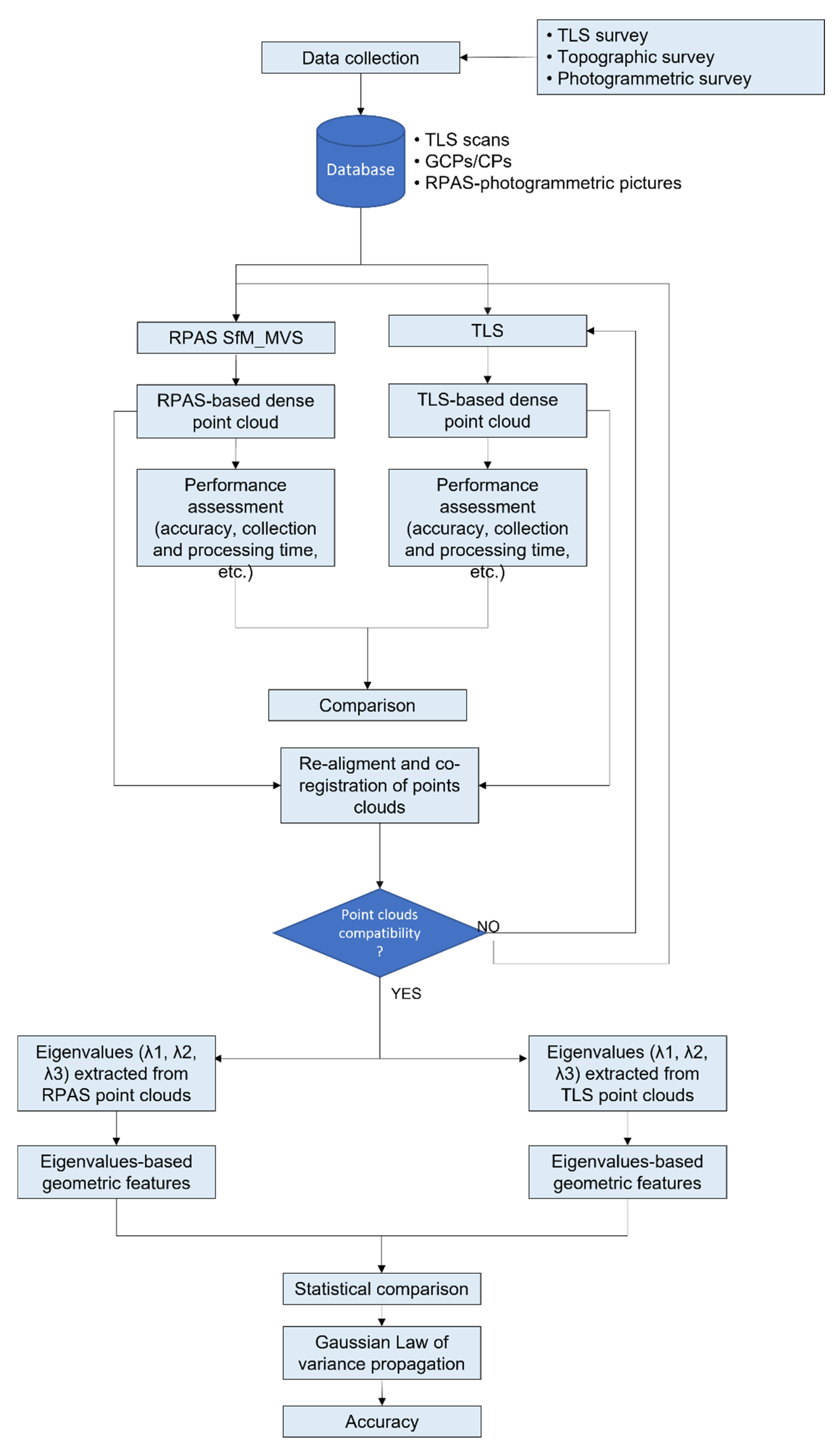
This section describes the methodology adopted to address the research goals, with the operative workflow outlined in Figure 1. Once the data collection phase was completed and the database built, photogrammetric pictures and TLS scans were handled separately, and their outcomes evaluated and compared. Lastly, after ensuring point cloud compatibility, eigenvalues-based geometric features were estimated, and their corresponding accuracy and reliability assessed.
2.1. Data Collection and Database Construction
Three flight campaigns were carried out over the experimental site on 18 April 2019 using a consumer quadcopter DJI Inspire 1 weighing 2.9 kg (payload included). This RPAS was equipped with a 3-axis gimbal to compensate for accidental vehicle movements, as well as a low-cost GNSS/INS positioning receiver to gather its position and the DJI Ground Station Pro app (Dà-Jiāng Innovations) [19] to set up and oversee the missions. All actions were performed at the same cruising speed (4.0 m/s) and altitude (25 m AGL, above ground level). According to the research of Dandois et al. (2015) [20], the STOP&GO flight mode was selected to reduce the number of blurry pictures collected using a DJI ZenMuse X3 camera, characterized by a focal length of 3.61 mm and a pixel size of 1.56 μm, mounted on the RPAS’ gimbal at both nadiral and 45° positions. Waypoint position was set to ensure the acquisition of both nadiral and oblique photogrammetric pictures, and thus, different longitudinal and transverse overlaps between them were established. Indeed, a longitudinal and transverse overlap of 90% was set to gather nadiral, while longitudinal and transverse overlaps of 90 and 70%, respectively, were selected to collect the oblique photos. Such a combination of flight and camera features ensured the collection of 202 aerial photogrammetric pictures with a nominal Ground Sample Distance (GSD) of 1.1 cm/pixel.
Simultaneously, an appropriate topographic survey was conducted to acquire the positions of 21 permanent natural elements on 20 December 2019. These points, homogeneously allocated overall to the pilot site, were surveyed using a Leica Geosystem GS18T receiver. Such a receiver was logged into the national network (National Dynamic Network RDN2008) of the Continuous Operation Reference Stations (CORS) through the permanent station in Valenzano (Bari) and the network Real-Time Kinematic (nRTK) acquisition mode was chosen. Ellipsoidal altitude points, stored up by the receiver, were further converted into orthometric altitude points with ConveRgo software [21], while RDN2008/UTM zone 33N (N-E) (EPSG: 6708) was selected as the Reference system. After their positions were collected, the data set was split into two respective categories composed of 11 and 10 points. Both of them were imported in Agisoft PhotoScan (v.1.4.1, Agisoft LLC -St. Petersburg, Russia) software [22], currently known as Metashape, which handled the RPAS-photogrammetric data and extracted accurate cloud points. The first group was adopted as Ground Control Points (GCPs) and the second one as Check Points (CPs) during the alignment phase of the gathered pictures.
Lastly, a Leica RTC360 3D Laser Scanner was adopted to acquire 34 scans of the study area on 29 November 2019. Such an instrument (recording capacity: 2,000,000 pts/sec, maximum range: 130 m, and range accuracy: 1.0 mm + 10 ppm) (Xiaohui et al. 2019) was set about 50 m away from the Monastery to also collect the dome data. Moreover, TLS scans were homogeneously collected at the All Saints’ Monastery of Cuti. The proprietary Leica Cyclone software (v.9.2.0) [23] was, thus, adopted to handle these data.
2.2. RPAS Digital Photogrammetry
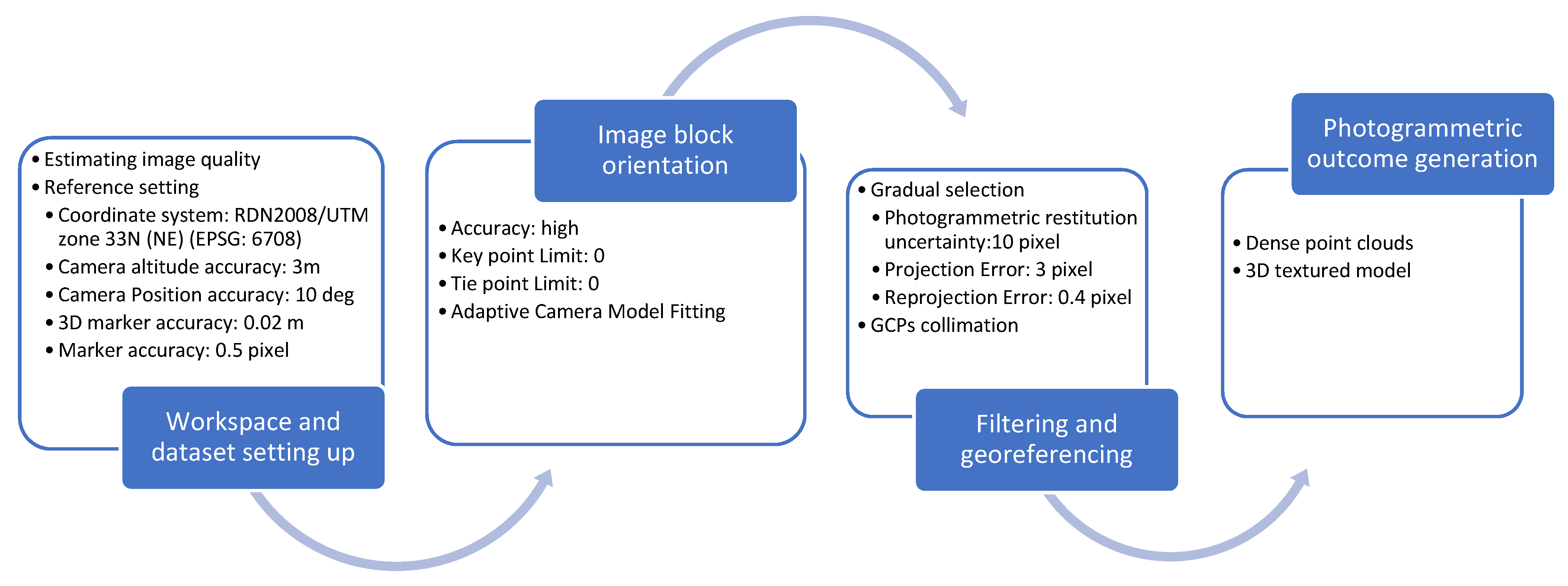
Figure 2 reports the procedure adopted to produce the RPAS-photogrammetric point cloud following the suggestions of Caroti et al. (2017) [24], Beretta et al. (2018) [25], and Manfreda et al. (2018) [26]. Specifically, the process was broken down into four key steps: (i) workspace and dataset setting up; (ii) image block orientation; (iii) filtering and georeferencing; and (iv) photogrammetric outcome generation.
Before importing the collected images into the Agisoft environment, they were checked over visually to detect and clean out the blurry ones, which could affect outcome accuracy. In addition, a quantitative evaluation of their quality was subsequently carried out by applying the “Estimate Image Quality” tool, which returns a value between 0 and 1 according to their sharpness, blurring, and distortion. Indeed, 0 was assigned to very poor-quality pictures while 1 was assigned to very high-quality ones [27,28,29,30,31]. In the present study, the useful images were selected using 0.6 as the threshold. After adequate images were selected, the workspace was arranged by fixing the values as reported in Figure 2. Specifically, the threshold of 3 m was assigned to the “Camera Positioning Accuracy” parameter to be consistent with the average 3D positioning accuracy value stored by the RPAS GNSS receiver, equal to 2.54 m. Conversely, the “Image Altitude Accuracy” was set as equal to 10 degrees because the RPAS-integrated Inertial Measurement Unit (IMU) did not provide any information on altitude measurements.
For the “Image block Orientation” step (second phase), aimed at the alignment of pictures and tie points detection, as pinpointed in Figure 2, the “High” accuracy mode was set with a threshold equal to 0 for the “Limits of Key Points and Tie Points” parameter, as recommended by Gruen and Beyer (2001) [30] and Triggs et al. (2000) [31]. This ensured no unchecked points filtering. After aligning the images and extracting the sparse point cloud, at the start of the third phase, named “Georeferencing and filtering”, three additional criteria were adopted to evaluate the systematic error and enhance the accuracy of the output. These criteria were as follows: (i) removal of all points characterized by low base–height ratios (ratio between the largest and smallest semiaxis of the error ellipse obtained by triangulating 3D point coordinates between two photos), such as those located on the edge of the images. This criterion was met by fixing the “Photogrammetric Restitution Uncertainty” parameter, which allows detecting the uncertainty in the position of a tie point based on the geometric relationship of the cameras from which that point was projected or triangulated, considering geometry and redundancy [22]; (ii) elimination of all less reliable points by setting a threshold equal to 3 as the “Projection Accuracy” parameter. Such a variable measures the “Mean Key Point Size”, defined as the standard deviation value of the Gaussian blur at the scale at which the point was detected [22]. This condition guarantees the exclusion of all tie points with uncertainty 3 times higher than the minimum one; and, lastly, (iii) a threshold of 0.4 was assigned to the “Reprojection Error” parameter (estimation of the error obtained by comparing a point’s original position on the image and the location of that point when it is re-projected to the photo [22]) in order to clean out all points characterized by a significant residual value. These threshold values were selected according to the recommendations by Saponaro et al. (2019a) [32]; Dandois et al. (2015) [20]; Gagliolo et al. (2018) [33]. This ensured the reduction of restitution errors and improvement of the orientation parameters. Indeed, by integrating the three abovementioned criteria, implemented in the “Gradual selection” tool, about 20% of the inaccurately estimated points from clouds were removed. Further improvement of georeferencing through the reduction of image block deformation resulted from uploading the GCPs in the Metashape software [34]. Thus, the dense point cloud was produced, and its accuracy was assessed by computing the root mean square error (RMSE) (phase 4—“Photogrammetric outcome generation”). The final output was imported into the CloudCompare environment for subsequent analysis [35].
2.3. TLS
Field scanning data collected using the Leica RTC360 3D Laser Scanner were im-ported into Leica Cyclone software where they were registered and georeferenced. This software was equipped with the “Registration module”, which allowed the automatic compensation for errors from the pre-registration procedure carried out during the data acquisition phase [36]. Thus, a total of 25 natural or artificial targets easily detectable in the clouds were picked as homologous points among the scans by using the Cloud Constraints Wizard tool [37]. This resulted in an average overlap of 46% among them. Before exploring the errors committed by computing the base statistics (mean, minimum, maximum, median, and quartile values), needless elements such as people and cars were filtered and cleaned out [3,4,5,6,7,8,9,10,11,12,13,14,15,16,17,18,19,20,21,22,23,24,25,26,27,28,29,30,31,32,33,34,35,36,37,38]. Lastly, all extracted point clouds were merged into a single one and exported as pts. This outcome was further investigated in the CloudCompare environment, which allowed extracting several geometric features useful to investigating the point clouds from several points of views [39].
2.4. Geometric Feature Extraction and 3D Point Cloud Accuracy Assessment
CloudCompare software provides a few plugins aimed at investigating point cloud accuracy and examining their spatial 3D information [32]. Because of this, the two resultant models were imported into that environment and thoroughly analyzed. Before proceeding in this direction, resultant cloud compatibility was also evaluated. The clouds were re-aligned and co-registered by pinpointing the GCPs in both models [3]. The TLS-based point cloud showed higher accuracy than the one obtained by surveying GCPs in nRTK mode and thus was used as a benchmark during the co-registration phase, as suggested by Fugazza et al. (2018) [40]. Subsequently, less accurate zones and points not depicting the pilot site were removed through the application of the Segment tool, implemented in the CloudCompare environment.
Hence, only the spatial information related to the case study was investigated during the subsequent steps through the computation of specific geometric features. Indeed, the 3D scene structure can be locally described by extracting the three eigenvalues (λ1, λ2 and λ3) of the 3D covariance matrix S, also known as the 3D structural tensor [41]. These eigenvalues express the dispersion relevance along their eigenvector and allow defining the structure typology: when λ1 » λ2, λ3, the structure is unidimensional, since the points are distributed along one main axis; while, when λ1 and λ2 » λ3 the structure is bidimensional because all the selected points are essentially arranged along two axes only; lastly, when λ1, λ2 and λ3 show similar values, the structure is tridimensional. S was estimated by considering the spatial information of all 3D points (X = (X, Y, Z)) within a local neighborhood V, defined by applying a sphere of a fixed radius rs [42]. The size of rs was determined in accordance with the proposal by Demantké et al. (2011) [43]. Thus, the radius was set as 0.05 m in accordance with the study area heterogeneity.
However, as recommended by West et al. (2004) [44] and Pauly et al. (2003) [45], the eigenvalues were not directly applied to explain the local structure at a point X; rather, a set of geometric features based on them (Linearity Lλ, Anisotropy Aλ, Sphericity Sλ, Planarity Pλ, Omnivariace Oλ, Curvature Cλ, Eigenvalues’ sum ∑λ) were computed. In the following, the formal definition of such parameters is reported:
Previous research studies proved that these factors are sensitive to noise [46,47,48], and therefore, the investigation of the robustness of the eigenvalues and relatives-based features deserve considerable attention. Indeed, as shown by Soudarissanane et al. (2011) [49], each individual 3D point experiences a random noise content owing to the influence of various factors. The methodology adopted to assess the accuracy and reliability of geometric features extracted from TLS and RPAS-based point clouds is thoroughly described in the next section.
The performance of the two resulting point clouds was firstly evaluated in terms of acquisition and processing time, number of points, and volume density. Indeed, as proposed by Jo and Hong (2019) [4] and Son et al. (2020) [3], the combination of such parameters allowed analyzing the homogeneity of point distribution. Volume density was estimated by using the “Cloud Density” tool implemented in the CloudCompare software. Their performance was then assessed by using the Multiscale Model-to-Model Cloud Comparison (M3C2) approach [39], which is based on two subsequent steps: the former, aimed at defining the normal point, and the latter intended to calculate the difference between the two considered point clouds. During the process, the normal scale and the maximum depth of the cylindrical projection were set as 0.10 and 0.5 m, respectively. The projection scale value (0.10 m) was instead chosen according to RPAS roughness, as suggested by Di Francesco et al. (2020) [50]. Indeed, this parameter strongly influenced the M3C2 output since selecting a too-small value enhances noise accumulation, while picking a too-high value hides the differences.
For each estimated distance, the M3C2 algorithm allowed also computing the Distance Uncertainty. A Level of Detection (LoD) equal to 95% was set to discriminate the statistically significant change in terms of distance between the two considered dense point clouds. Thus, the distance was statically significant when it was higher than the LoD95% value, computed by applying Equation (8).
σ1(d)2 and σ2(d)2 are the variances of the two clouds’ positions, while n1 and n2 are the numbers of points of RPAS- and TLS-extracted clouds, respectively. Lastly, reg represents the co-registration error between the two considered dense point clouds. The outcome of this procedure was used as a benchmark to evaluate the accuracy.
2.5. The Gaussian Law of Variance Propagation
As mentioned in the previous section, each 3D point is subjected to noise mainly from the survey instrument, terrain heterogeneity, and scanning geometry [49], which translates into an error in the planimetric and altitude coordinate values definition expressed as the standard deviations related to each component (σx, σy, σz). Nevertheless, their values are not homogeneous over the entire 3D structure since each individual point can show a different deviation standard. The variance of a function f (f = f (x1, …, xn)) of random variables xi can be appreciated through the application of the variance propagation law. Commonly, the Taylor series, reported in Equation (9), was adopted to address such a purpose.
Generally, only the first-order term is adopted to model the error because of the irrelevant effect of all higher order terms on the variance propagation, as shown by Dittrich et al. (2017) [15]. Thus, Equation (9) is simplified as follows:
Thus, it is expressed as:
When n > 1, Equation (12) is modified as follows:
Assuming all variables as mutually independent and squaring Equation (13), the Gaussian law of variance propagation of function f is obtained:
By applying the Gaussian law of variance propagation at the 3D structure tensor, the variances of the abovementioned features, described by Equations (1)–(7), are expressed as follows [15]:
See Dittrich et al. (2017) [15] for more details concerning the application of the Gaussian law of variance propagation at the 3D structure tensor. A proper code in the R environment was developed to implement the Gaussian law of variance propagation and to estimate the geometric features accuracy. It was separately applied on TLS and RPAS-based geometric features. Lastly, the outputs of both procedures were compared.
3. Case Study
The All Saints’ Monastery of Cuti (Figure 3), located 2 km away from the city center of Valenzano (Bari, Southern Italy), was selected as the case study of this research both for its historical and architectural relevance and for the current intention of the municipality of Valenzano to support local tourism. It was built by the priest Eustazio together with a group of monks between 1080 and 1083 to provide the people living in the countryside surrounding Bari with a Catholic place of prayer. Despite its abandonment in 1811, the demolition of two cloisters, and the addition of extra elements, i.e., two bell towers and boundary walls, the Monastery is still considered one of the few remaining well-conserved Apulian Romanesque architecture examples [51]. Indeed, it is a hall church with domes on the axis, a typical structure of Apulian architecture since the 7th century [50]. Its external part consists of three domes in line with the central nave and an incomplete portico that only partially covers the church. The central dome is the highest and widest. Its interior part is divided into three naves with a half-barrel vault. Unfortunately, most of the original furnishings and liturgical vestments have been lost over the years [50]. RPAS-photogrammetric, topographic, and TLS surveys were separately conducted to generate its 3D representation, as previously described.
4. Results and Discussion
Two dense point clouds reflecting the All Saints’ Monastery of Cuti, located in the province of Bari, were generated [50]. The former was extracted by handling 202 RPAS-photogrammetric photos, including both nadiral and oblique pictures, while the latter was obtained by processing 24 TLS scans. The remaining 10 scans were not included during the processing step since they referred to the interior of the Monastery. Firstly, the results of these techniques were compared in terms of the time needed to collect and process the data. As highlighted in Table 1, TLS seemed to be a more affordable tool to produce 3D scene reconstruction thanks to the shorter data processing time (450 versus 978 min) albeit the acquiring time was about 136 min more. The time needed to measure GCPs and CPs, equal to 40 min, was added to the abovementioned acquisition time. This kind of evaluation depended on computer performance. An Intel® CoreTM i7-3970X CPU @3.50GHz with 16 GB RAM was applied in this case.
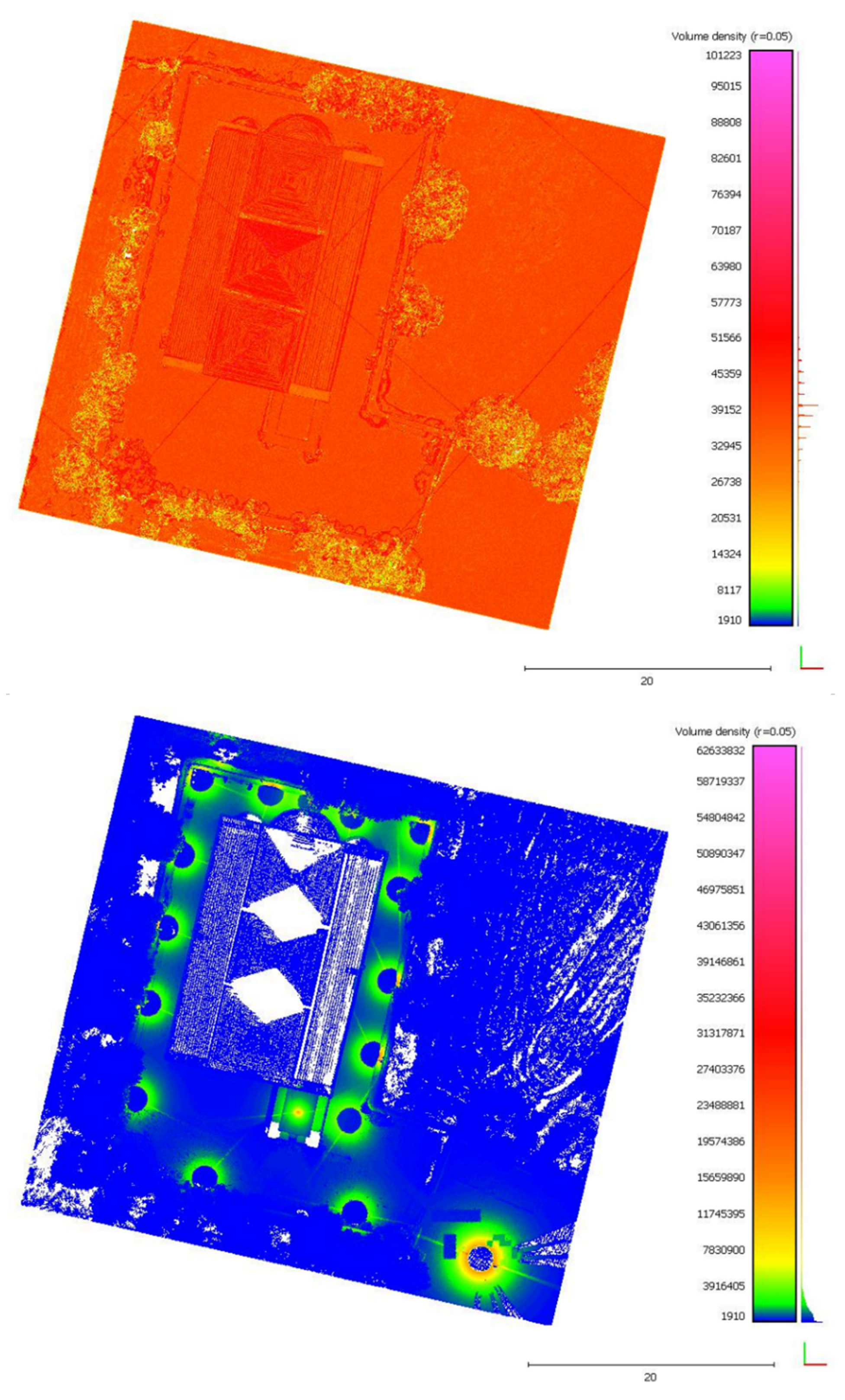
This parameter was not enough to assess the performance of the two techniques, and thus, additional proprieties such as volume density and number of points were in-volved. TLS returned a higher number of points (195,939,535 versus 28,202,789) (Table 1), which should have resulted in a higher-detailed reproduction of the Monastery geometry. However, the corresponding 3D point cloud was heavy and hard to oversee and manage. Therefore, as proposed by Son et al. (2020) [3] and already explained in Section 2.3, it was further filtered to drastically reduce point numerosity. Nonetheless, the resultant cloud was still denser than that one produced using RPAS-photogrammetry (191,519,447 versus 28,202,789) (Table 1). This parameter was not significant enough to define the 3D reconstruction effectiveness and reliability. As a consequence, point distribution homogeneity was investigated by estimating the volume density parameter, as suggested by Jo and Hong (2019) [4] and Son et al. (2020) [3]. Figure 4 reports volume density outcomes for both models. Although the volume density parameter was higher for the TLS-based model than the RPAS-based one, a lack of data related to the ground and the central part of the roof can be detected. Such a loss of data, depicted in white in Figure 4, made it impossible to reconstruct that area using only TLS data. As previously observed by Lague et al. (2013) [39] and Di Francesco et al. (2020) [50], point inhomogeneity in the TLS cloud was mainly caused by the distance between the Monastery and the instrumental standpoint. The combination of the inhomogeneous distribution of points and the lack of data impacted on the quality of the final 3D reconstruction. In contrast, the RPAS model generated a homogenous point distribution over all the study area thanks to the integration of nadiral and oblique photos. This ensured the generation of a consistent 3D reconstruction both horizontally and vertically. Nevertheless, its output quality was affected by the user’s skill in acquiring and handling data [50]. Both model outcomes did not experience significant blockages and, therefore, the vertical facades were totally reconstructed.
The two techniques were also compared in terms of the accuracy of the generated 3D digital representations. Thus, basic statistics metrics were estimated for the two resultant models. Mean, Maximum, and Minimum Error (ME, Max, and Min) values were calculated for the TLS-based reconstruction. Their values were equal to 0.004, 0.017, and 0.001 m, respectively. Median, 1st, and 3rd quartiles were computed as well. Their values were equal to 0.002, 0.001, and 0.003 m. Conversely, base statistics metrics related to the RPAS-based model are reported in Table 2. The root mean square error (RMSE) estimated on GCPs evaluated the Bundle Block Adjustment (BBA) phase accuracy, while the ones computed on CPs assessed the accuracy of the final product. The errors committed on each axis (RMSEx, RMSEy, and RMSEz) and the total errors (RMSET) are reported in Table 2. 3D reconstruction generated by handling TLS data was slightly more accurate than the one produced by processing RPAS input data.
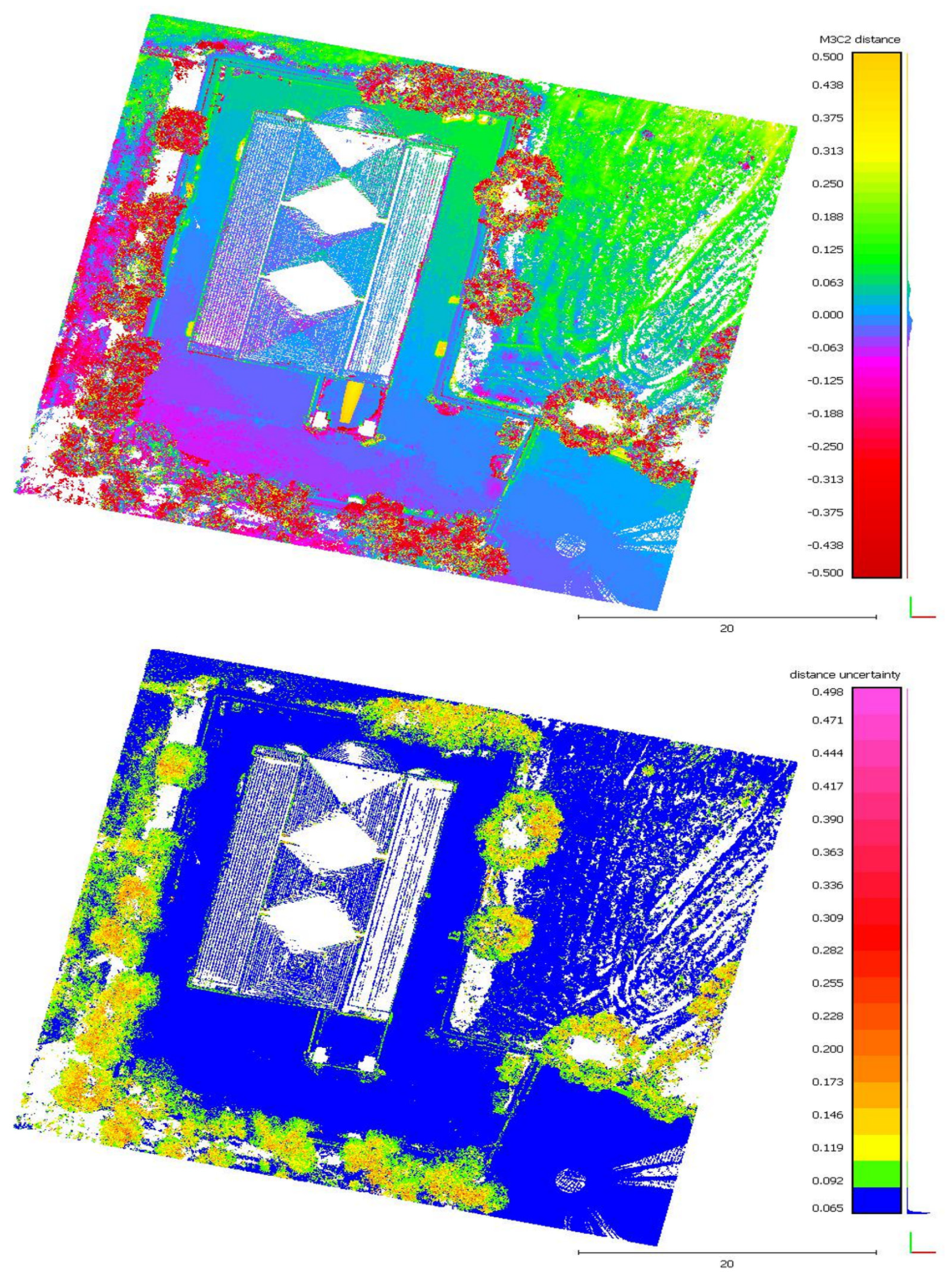
Lastly, cloud-to-cloud distance was also evaluated through the application of the M3C2 tool of CloudCompare. As previously, the most significant divergences were located on the vegetated areas and on the roof (Figure 5). This was essentially caused by the lack of data in the TLS-based model, as already highlighted in the previous paragraphs. Excluding those areas, the M3C2 outcome showed a value comprised between −0.063 and 0.005 m on the horizontal and vertical facades of the Monastery, and between −0.2 and −0.1 m on the portal and rose window. The precision of this measurement was instead evaluated by computing M3C2 Uncertainty, with results reported in Figure 5. M3C2 Uncertainty was between 0.065 and 0.085 m and between 0.09 and 0.146 m for the Monastery structure and the green areas, respectively. This comparison ensured full compatibility among the obtained reconstructs and highlighted the weakness of each applied approach, already noted in the previous paragraph. No specific issues were detected by performing that analysis.
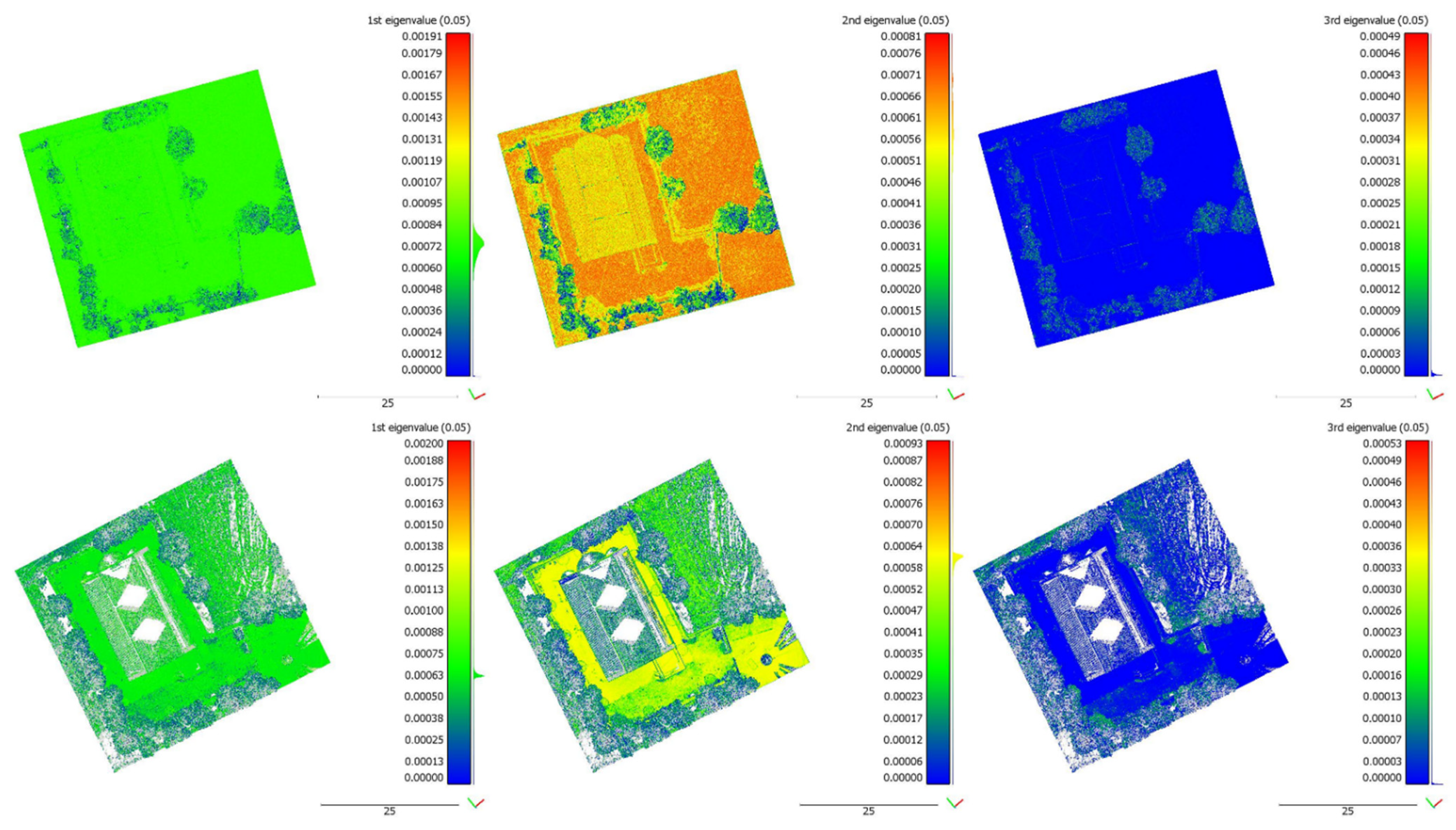
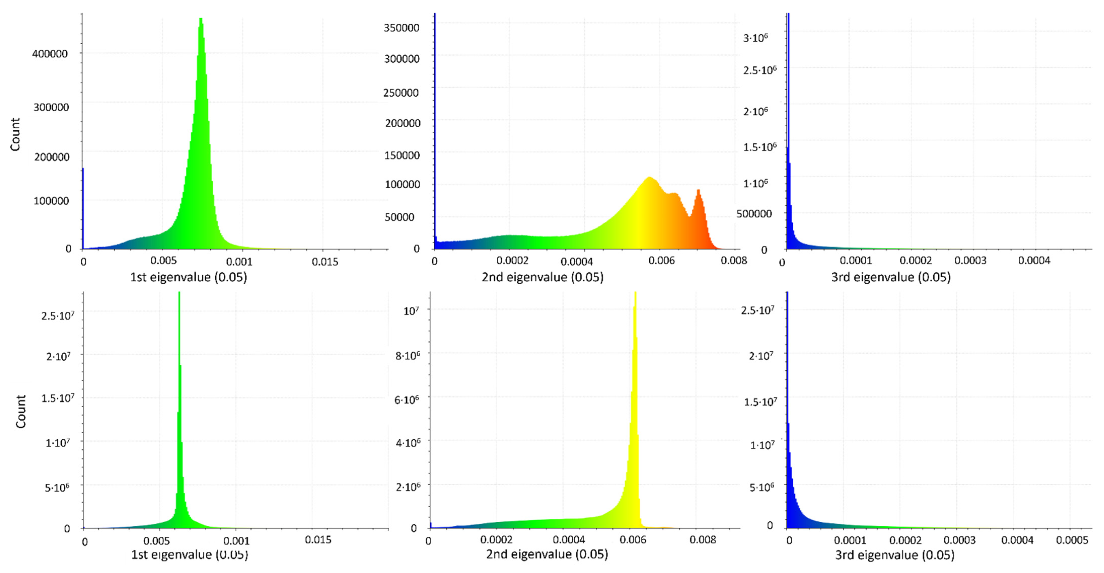
A further investigation concerning the resultant models was performed by extracting the corresponding geometric features and their accuracy, as detailed in Section 2.5. Thus, the three eigenvalues (λ1, λ2 and λ3) of the 3D covariance matrix S were extracted from TLS and RPAS dense point clouds (Figure 6). To easily compare their values, the corresponding histograms were computed and are reported in Figure 7. λ1, λ2 and λ3 values were within the same order of magnitude for both models albeit the number of points were different for the two resultant clouds, as previously highlighted. Moreover, λ1 and λ3 had the same trend in contrast to the second eigenvalue, which showed a more complex distribution of around 0.0007 for the TLS-based model compared to the RPAS one. This indicated that the size and the shape of the point clouds generated by RPAS and TLS were similar along the most elongated direction (identified by λ1) as well as along the “flat” dimension (defined by λ3). Conversely, some divergences were detected along the second elongation direction (underlined by λ2). As depicted in Figure 6, these differences are mainly located on the vegetated areas and on the ground, and thus, they did not affect the point clouds’ performance in the area under investigation. This indicated that no significant differences were detected among them.
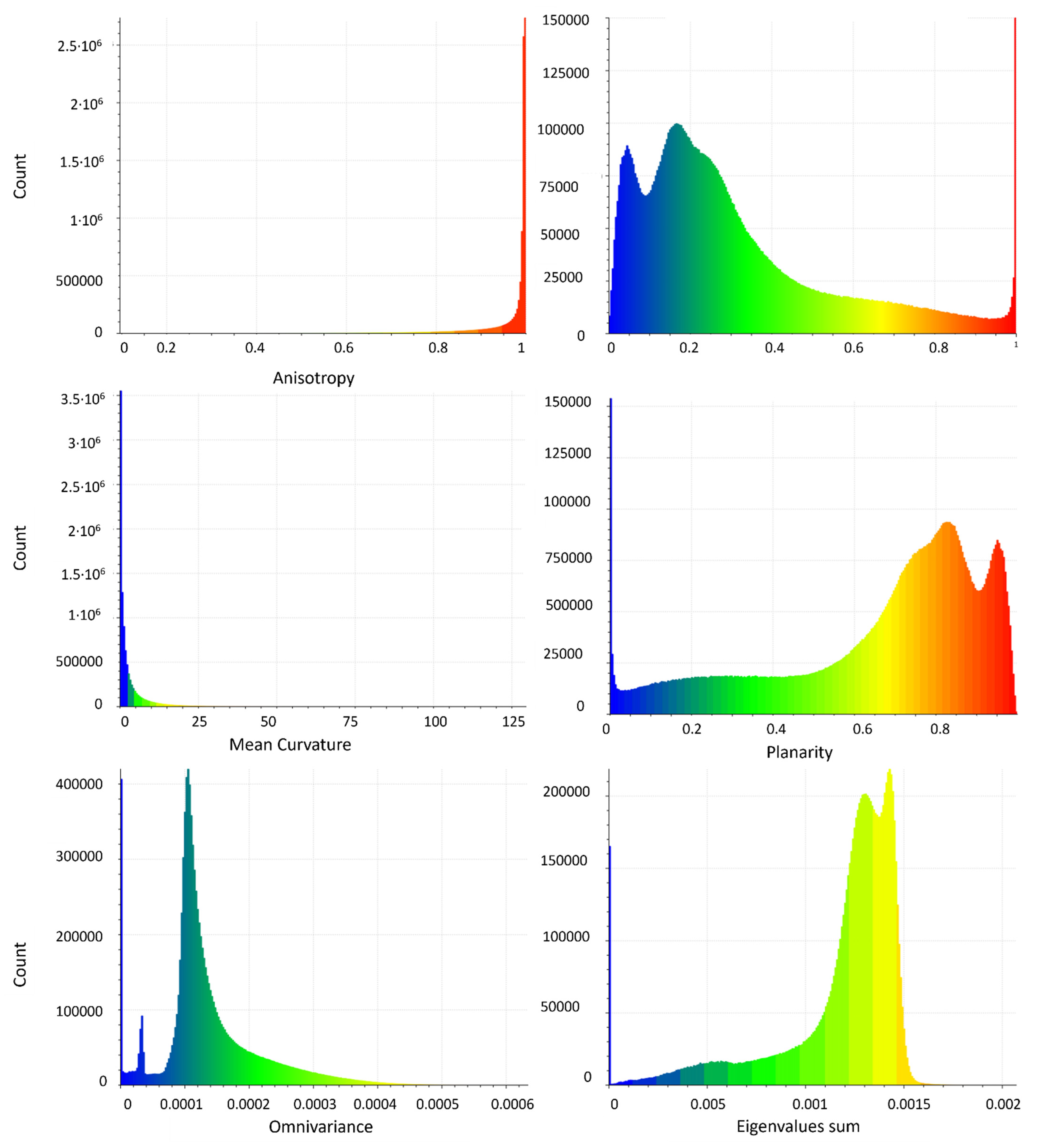
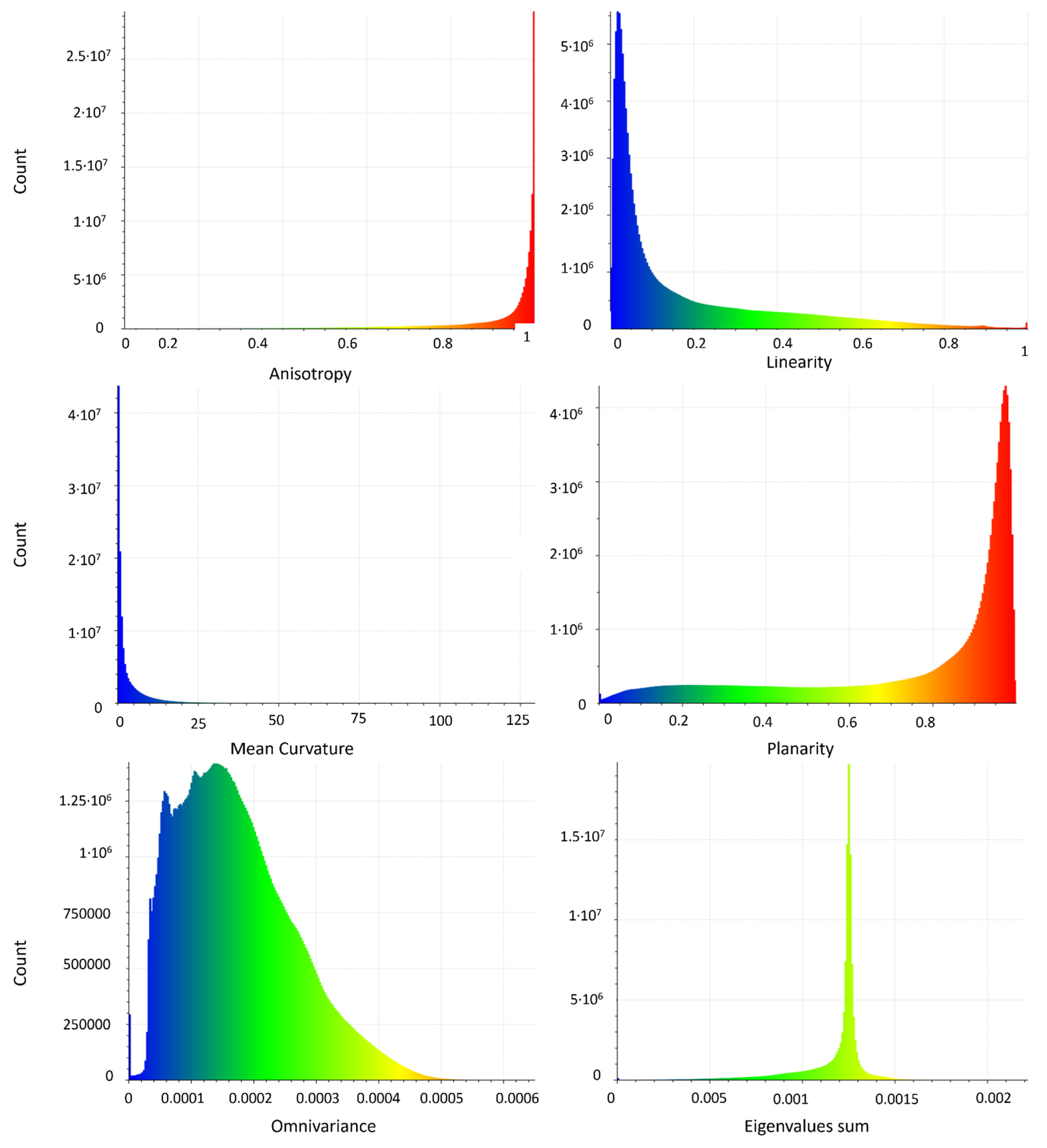
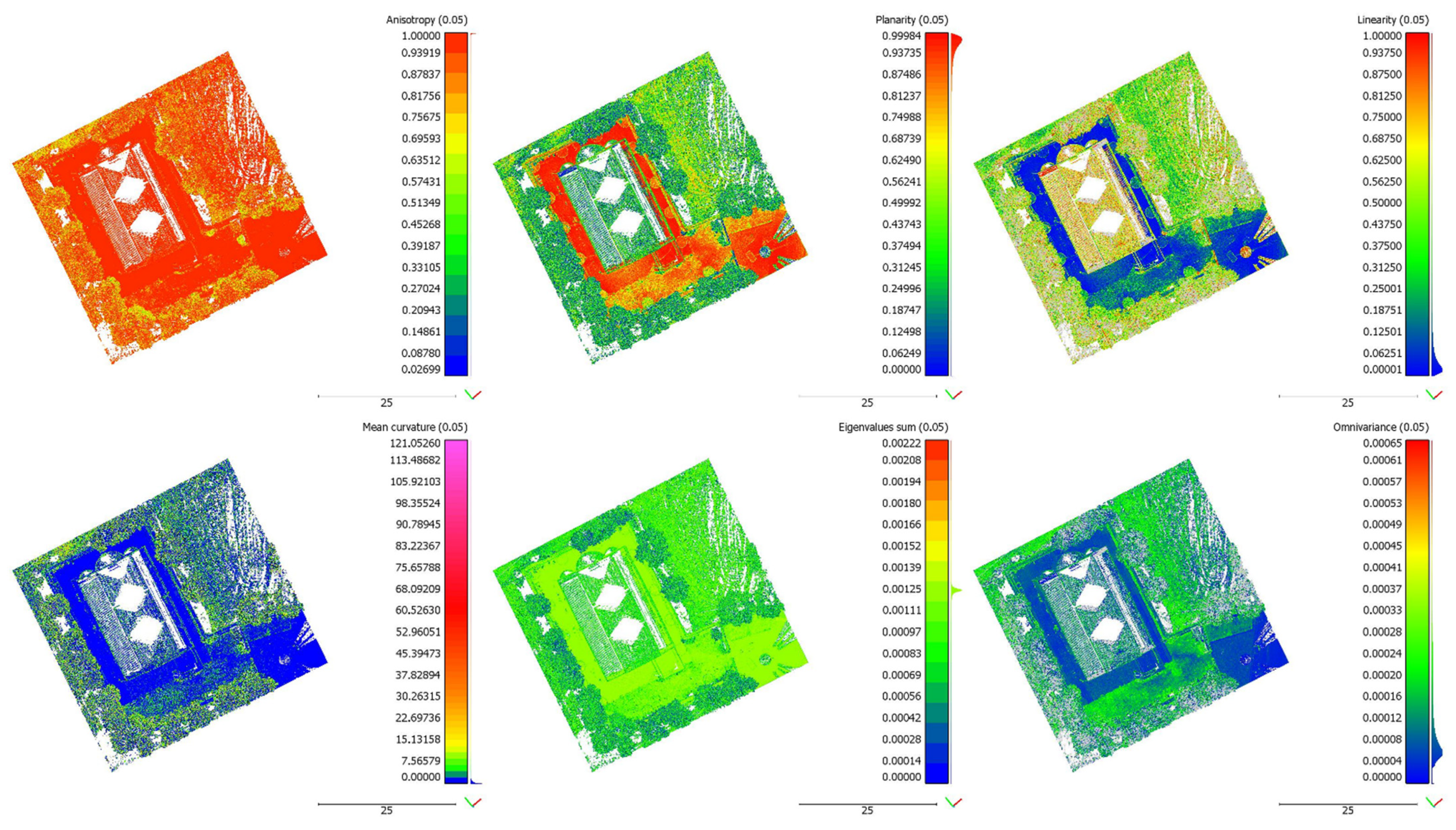
Generally, covariance features are used more often than raw eigenvalues for 3D structure investigations and point cloud classification purposes [17,44]. Therefore, as explained in Section 2.5, eigenvalues-based geometric features and their corresponding variances were assessed as well. Histograms of these properties referring to the RPAS and TLS models are depicted in Figure 8 and Figure 9, respectively. Although all features were in the same order of magnitude, anisotropy, curvature, and sphericity showed similar trends in both models, in contrast to the remaining features (omnivariance, linearity, rigenvalue sum, and planarity). The latter are detailed in Figure 10 and Figure 11, which illustrate that the differences are essentially from the lack of data on the ground and on the vegetated areas in the TLS model. Moreover, Figure 10 and Figure 11 highlight that the RPAS-based point cloud was less affected by noise, and thus, the obtained features were easier to interpret and manage. This indicated that the RPAS dense point cloud was more stable and consistent.
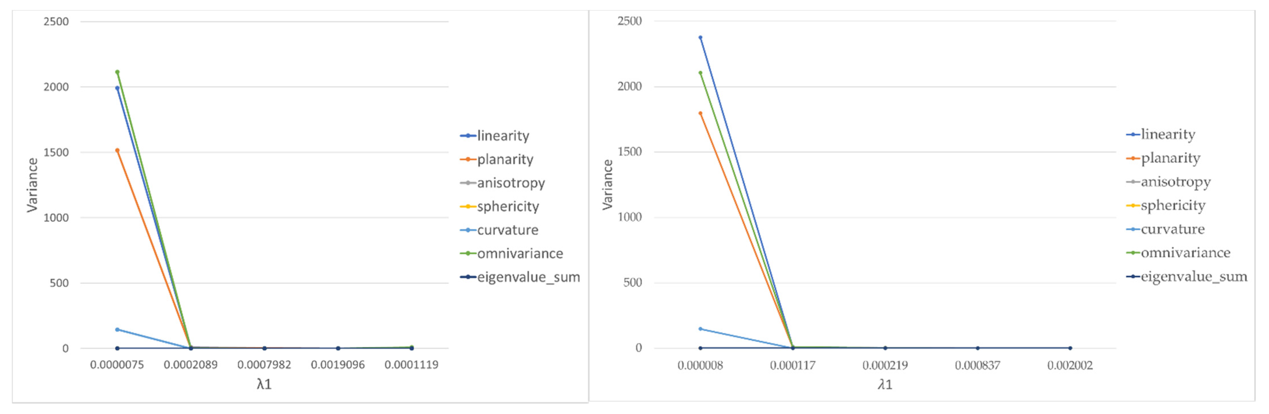
Lastly, the variance of the geometric features extracted from the RPAS-based and TLS-based models was separately estimated by applying the Gaussian law of variance propagation [15]. The outcome of this analysis is reported in Figure 12, which describes the trend of geometric features variance as a function of λ1. The features trends as a function of λ2 and λ3 were nearly similar and, thus, only the values according to λ1 variation were reported. The variance contribution was significant at low values for all examined properties, except linearity, curvature, and omnivariance were the most affected by that noise. In particular, as to the linearity, the variance effect was more evident in the RPAS model than in the TLS model. As previously stated, in both models the low values of λ1 corresponded to the vegetation, considered to be the noisiest and least accurate zone. This indicated that the noise particularly affected the vegetated areas. In contrast, the noise impact was less relevant in accordance with the increment of λ1 values.
Thus, the Gaussian law of variance propagation underlined the noise impact on the eigenvalues-based geometric features. This implied that all considered geometric features were mainly corrupted by the noise at low values of the eigenvalues. Thus, specific attention should be paid to these areas, which may require a further filtering analysis before the classification procedure. In the investigated case, these areas were not linked to the All Saints’ Monastery of Cuti, and as a consequence, they were not properly filtered.
5. Conclusions
This paper assessed TLS and RPAS digital photogrammetry approaches to reproducing accurate 3D scene reconstruction of a cultural heritage building. Specifically, after investigating the performance of the two abovementioned approaches, geometric features were extracted from both resultant models and evaluated. This analysis was carried out on the All Saint Monastery, located in Valenzano (Bari, Southern Italy), selected as the pilot site for this study because of its historical and architectural relevance.
The area under investigation was inspected by applying three different geomatic techniques: a topographic survey to collect GCPs and CPs, a photogrammetric method to gather photogrammetric photos using an RPAS, and lastly a TLS acquisition. RPAS SfM-MVS and TLS approaches are widely used to reproduce a cultural heritage building with accuracy because of their ease of use and high level of automation. However, both techniques had pros and cons and, thus, their limits and benefits were compared and discussed. The main divergences between the abovementioned methods are as follows:
- RPAS allowed reducing the time required to collect the input data while TLS permitted generating the final 3D model in a shorter operational time;
- The RPAS-based point cloud was less dense than the one produced by TLS and thus more easily manageable;
- The point distribution of the TLS-derived cloud was not homogeneous and, consequently, the accuracy of the 3D reconstruction was not uniform in the final model;
- RPAS allowed surveying the entire study area while TLS did not permit the collection of data concerning the roof of the Monastery, the vegetated areas, and the grounds;
- RPAS was a low-cost tool while TLS was a highly expensive instrument.
Thus, although two accurate 3D digital representations were produced, both point clouds showed several limitations, mainly from the lack of data in relation to the roof of the Monastery, the vegetated areas, and the grounds in the TLS outcome as well as the low point numerosity in the RPAS cloud. Additionally, the RPAS-based point cloud was obtained by using Metashape, a commercial user-friendly software that enables 3D scene reproduction with camera self-calibration. Although this was an undeniable advantage in terms of saving processing time, it resulted in a decrement of the accuracy of the generated 3D model. Such an error level was in part reduced by the introduction of GNSS measurement during the BBA phase. As a result, the 3D scene representation was only partial in the case of the TLS model, and it was less reliable in the case of the RPAS-based model. This indicated that neither of the two outcomes could be considered an effective reconstruction of the examined physical asset.
Nevertheless, point clouds are commonly applied to meet classification purposes and structure investigation. Thus, the eigenvalues-based geometric features and the propagated variance were also inspected. All point clouds are affected by noise, mainly from the survey instrument, terrain heterogeneity, and scanning geometry. The noise, however, was not homogeneous overall in the generated models and, thus, a critical analysis of its distribution appeared essential to detect and reduce errors and uncertainty levels. The Gaussian law of variance propagation approach to the point cloud-derived products allowed meeting such a purpose. Indeed, assessing the variance trend involved detecting the noise influence on the final model and geometric features reliability. Both models showed similar trends for all eigenvalues-based geometric features: the variance contribution was higher at low values. Nevertheless, linearity, curvature and omnivariance were most affected by the noise and, thus, could not be considered stable. Thus, no significant differences in variance were detected between the models. Only the trend of the linearity variance was slightly different. Further investigations are required to generalize these results and to quantify the contribution of such a procedure to classification output.
In conclusion, although the RPAS-based 3D reconstruction was less accurate than that extracted by adopting the TLS, it allowed representing the scene entirely and computing consistent and reliable geometric features useful for addressing classification purposes. The use of the Gaussian law of variance propagation approach appears promising to detect the noise impact on eigenvalues-based geometric features before performing a subsequent classification procedure.
Funding
This research was conducted within the project “Programma Operativo Nazionale Ricerca e Innovazione 2014-2020—Fondo Sociale Europeo, Azione I.2 “Attrazione e Mobilità Internazionale dei Ricercatori”—Avviso D.D. n 407 del 27/02/2018” CUP: D94I18000220007—cod. AIM1895471—2.
Institutional Review Board Statement
Not applicable.
Informed Consent Statement
Not applicable.
Conflicts of Interest
The author declares no conflict of interest.
Abbreviation
| 3D | Three-Dimensional |
| AGL | Above Ground Level |
| BBA | Bundle Block Adjustment |
| CORS | Continuous Operation Reference Stations |
| CPs | Check Points |
| EPSG | European Petroleum Survey Group |
| GCPs | Ground Control Points |
| GNSS | Global Navigation Satellite System |
| GSD | Ground Sample Distance |
| IMU | Inertial Measurement Unit |
| INS | Inertial Navigation System |
| LoD | Level of Detection |
| M3C2 | Model-to-Model Cloud Comparison |
| MSV | MultiView Stereo |
| nRTK | Network Real-Time Kinematic |
| RMSE | Root Mean Square Error |
| RPAS | Remotely Piloted Aircraft Systems |
| SfM | Structure from Motion |
| TLS | Terrestrial Laser Scanner |
| v. | version |
References
- El-Hakim, S.F.; Beraldin, J.A.; Picard, M.; Godin, G. Detailed 3D reconstruction of large-scale heritage sites with integrated techniques. IEEE Comput. Graph. Appl. 2004, 24, 21–29. [Google Scholar] [CrossRef]
- Remondino, F. Heritage recording and 3D modeling with photogrammetry and 3D scanning. Remote Sens. 2011, 3, 1104–1138. [Google Scholar] [CrossRef] [Green Version]
- Jo, Y.H.; Hong, S. Three-dimensional digital documentation of cultural heritage site based on the convergence of terrestrial laser scanning and unmanned aerial vehicle photogrammetry. ISPRS Int. J. Geo-Inf. 2019, 8, 53. [Google Scholar] [CrossRef] [Green Version]
- Son, S.W.; Kim, D.W.; Sung, W.G.; Yu, J.J. Integrating UAV and TLS Approaches for Environmental Management: A Case Study of a Waste Stockpile Area. Remote Sens. 2020, 12, 1615. [Google Scholar] [CrossRef]
- Colomina, I.; Molina, P. Unmanned aerial systems for photogrammetry and remote sensing: A review. ISPRS J. Photogramm. Remote Sens. 2014, 92, 79–97. [Google Scholar] [CrossRef] [Green Version]
- Palladino, M.; Nasta, P.; Capolupo, A.; Romano, N. Monitoring and modelling the role of phytoremediation to mitigate non-point source cadmium pollution and groundwater contamination at field scale. Ital. J. Agron. 2018, 13 (Suppl. 1), 59–68. [Google Scholar]
- Luhmann, T.; Chizhova, M.; Gorkovchuk, D. Fusion of UAV and Terrestrial Photogrammetry with Laser Scanning for 3D Reconstruction of Historic Churches in Georgia. Drones 2020, 4, 53. [Google Scholar] [CrossRef]
- Rangel, J.M.G.; Gonçalves, G.R.; Pérez, J.A. The impact of number and spatial distribution of GCPs on the positional accuracy of geospatial products derived from low-cost UASs. Int. J. Remote Sens. 2018, 39, 7154–7171. [Google Scholar] [CrossRef]
- Padró, J.C.; Muñoz, F.J.; Planas, J.; Pons, X. Comparison of four UAV georeferencing methods for environmental monitoring purposes focusing on the combined use with airborne and satellite remote sensing platforms. Int. J. Appl. Earth Obs. Geoinf. 2019, 75, 130–140. [Google Scholar] [CrossRef]
- Mesas-Carrascosa, F.J.; Torres-Sánchez, J.; Clavero-Rumbao, I.; García-Ferrer, A.; Peña, J.M.; BorraSerrano, I.; López-Granados, F. Assessing optimal flight parameters for generating accurate multispectral orthomosaicks by UAV to support site-specific crop management. Remote Sens. 2015, 7, 12793–12814. [Google Scholar] [CrossRef] [Green Version]
- Saponaro, M.; Capolupo, A.; Caporusso, G.; Borgogno Mondino, E.; Tarantino, E. Predicting the Accuracy of Photogrammetric 3D Reconstruction from Camera Calibration Parameters through a Multivariate Statistical Approach. In Proceedings of the XXIV ISPRS Congress, Nice, France, 4–10 July 2020; ISPRS: Hannover, Germany, 2020; Volume 43, pp. 479–486. [Google Scholar]
- Capolupo, A.; Saponaro, M.; Borgogno Mondino, E.; Tarantino, E. Combining Interior Orientation Variables to Predict the Accuracy of RPAS–SFM 3D Models. Remote Sens. 2020, 12, 2674. [Google Scholar] [CrossRef]
- Lumban-Gaol, Y.A.; Murtiyoso, A.; Nugroho, B.H. Investigations on the bundle adjustment results from SFM-based software for mapping purposes. Int. Arch. Photogramm. Remote Sens. Spat. Inf. Sci. 2018, 42, 623–628. [Google Scholar] [CrossRef] [Green Version]
- Weinmann, M.; Jutzi, B.; Mallet, C. Feature relevance assessment for the semantic interpretation of 3D point cloud data. ISPRS Ann. Photogramm. Remote Sens. Spat. Inf. Sci. 2013, II-5/W2, 313–318. [Google Scholar] [CrossRef] [Green Version]
- Dittrich, A.; Weinmann, M.; Hinz, S. Analytical and numerical investigations on the accuracy and robustness of geometric features extracted from 3D point cloud data. ISPRS J. Photogramm. Remote Sens. 2017, 126, 195–208. [Google Scholar] [CrossRef]
- Chehata, N.; Guo, L.; Mallet, C. Airborne LIDAR feature selection for urban classification using random forests. Int. Arch. Photogramm. Remote Sens. Spat. Inf. Sci. 2009, 38 Pt 3/W8, 207–212. [Google Scholar]
- Mallet, C.; Bretar, F.; Roux, M.; Soergel, U.; Heipke, C. Relevance assessment of full-waveform lidar data for urban area classification. ISPRS J. Photogramm. Remote Sens. 2011, 66, S71–S84. [Google Scholar] [CrossRef]
- Maas, H.-G.; Vosselman, G. Two algorithms for extracting building models from raw laser altimetry data. ISPRS J. Photogramm. Remote Sens. 1999, 54, 153–163. [Google Scholar] [CrossRef]
- DJI. Dà-Jiāng Innovations. 2020. Available online: https://www.dji.com (accessed on 11 December 2019).
- Dandois, J.P.; Olano, M.; Ellis, E.C. Optimal altitude, overlap, and weather conditions for computer vision UAV estimates of forest structure. Remote Sens. 2015, 7, 13895–13920. [Google Scholar] [CrossRef] [Green Version]
- Cima, V.; Carroccio, M.; Maseroli, R. Corretto utilizzo dei Sistemi Geodetici di Riferimento all’interno dei software GIS. In Proceedings of the Atti 18a Conferenza Nazionale ASITA, Firenze, Italy, 14–16 October 2014; pp. 359–363. [Google Scholar]
- Agisoft LLC. Agisoft Metashape User Manual—Professional Edition, Version 1.6; Agisoft LLC: St. Petersburg, Russia, 2020; pp. 1–172. Available online: https://www.agisoft.com/pdf/metashape-pro_1_6_en.pdf (accessed on 22 January 2021).
- Wang, X.; Wu, X. Application of Leica RTC360 3D laser scanner in completion survey. Bull. Surv. Mapp. 2019, 10, 150. [Google Scholar]
- Tong, X.; Liu, X.; Chen, P.; Liu, S.; Luan, K.; Li, L.; Liu, S.; Liu, X.; Xie, H.; Jin, Y.; et al. Integration of UAV-based photogrammetry and terrestrial laser scanning for the three-dimensional mapping and monitoring of open-pit mine areas. Remote Sens. 2015, 7, 6635–6662. [Google Scholar] [CrossRef] [Green Version]
- Beretta, F.; Shibata, H.; Cordova, R.; Peroni, R.D.L.; Azambuja, J.; Costa, J.F.C.L. Topographic modelling using UAVs compared with traditional survey methods in mining. REM Int. Eng. J. 2018, 71, 463–470. [Google Scholar] [CrossRef]
- Caroti, G.; Piemonte, A.; Nespoli, R. UAV-Borne photogrammetry: A low-cost 3D surveying methodology for cartographic update. MATEC Web Conf. 2017, 120, 09005, EDP Sciences. [Google Scholar] [CrossRef] [Green Version]
- Manfreda, S.; McCabe, M.F.; Miller, P.E.; Lucas, R.M.; Madrigal, V.P.; Mallinis, G.; Ben Dor, E.; Helman, D.; Estes, L.; Ciraolo, G.; et al. On the Use of Unmanned Aerial Systems for Environmental Monitoring. Remote Sens. 2018, 10, 641. [Google Scholar] [CrossRef] [Green Version]
- Daakir, M.; Pierrot-Deseilligny, M.; Bosser, P.; Pichard, F.; Thom, C.; Rabot, Y. Study of lever-arm effect using embedded photogrammetry and on-board GPS receiver on UAV for metrological mapping purpose and proposal of a free ground measurements calibration procedure. ISPRS Ann. Photogramm. Remote Sens. Spat. Inf. Sci. 2016, XL-3/W4, 65–70. [Google Scholar] [CrossRef] [Green Version]
- James, M.R.; Robson, S.; d’Oleire-Oltmanns, S.; Niethammer, U. Optimizing UAV topographic surveys processed with structure-from-motion: Ground control quality, quantity and bundle adjustment. Geomorphology 2017, 280, 51–66. [Google Scholar] [CrossRef] [Green Version]
- Gruen, A.; Beyer, H.A. System calibration through self calibration. In Calibration and Orientation of Cameras in Computer Vision; Gruen, A., Huang, T.S., Eds.; Springer: New York, NY, USA, 2001; pp. 163–194. [Google Scholar]
- Triggs, W.; McLauchlan, P.; Hartley, R.; Fitzgibbon, A. Bundle adjustment—A modern synthesis. In Vision Algorithms: Theory and Practice; Triggs, W., Ziesserman, A., Sterliski, R., Eds.; Springer: Berlin/Heidelberg, Germany, 2000; pp. 298–375. [Google Scholar]
- Saponaro, M.; Capolupo, A.; Tarantino, E.; Fratino, U. Comparative Analysis of Different UAV-Based Photogrammetric Processes to Improve Product Accuracies. In Proceedings of the International Conference on Computational Science and Its Applications, St. Petersburg, Russia, 1–4 July 2019; Springer: Cham, Switzerland, 2019; pp. 225–238. [Google Scholar]
- Gagliolo, S.; Fagandini, R.; Passoni, D.; Federici, B.; Ferrando, I.; Pagliari, D.; Pinto, L.; Sguerso, D. Parameter optimization for creating reliable photogrammetric models in emergency scenarios. Appl. Geomat. 2018, 10, 501–514. [Google Scholar] [CrossRef]
- Saponaro, M.; Tarantino, E.; Fratino, U. Generation of 3D surface models from UAV imagery varying flight patterns and processing parameters. AIP Conf. Proc. 2019, 2116, 280009, AIP Publishing LLC. [Google Scholar]
- Girardeau-Montaut, D. Cloud Compare—3D Point Cloud and Mesh Processing Software; Open Source Project. Available online: http://www.danielgm.net/cc/ (accessed on 20 March 2020).
- Costantino, D.; Angelini, M.G.; Caprino, G. Laser scanner survey of an archaeological site—Scala di Furno (Lecce, Italy). In Proceedings of the ISPRS Commission V, Mid-Term Symposium “Close Range Image Measurements Techniques”, Newcastle upon Tyne, UK, 21–24 June 2010; Volume XXXVIII Part 5, pp. 178–183. [Google Scholar]
- Capolupo, A.; Maltese, A.; Saponaro, M.; Costantino, D. Integration of terrestrial laser scanning and UAV-SFM technique to generate a detailed 3D textured model of a heritage building. In Earth Resources and Environmental Remote Sensing/GIS Applications XI; International Society for Optics and Photonics: Bellingham, WA, USA, 2020; Volume 11534, p. 115340Z. [Google Scholar]
- Ozimek, A.; Ozimek, P.; Skabek, K.; Łabędź, P. Digital modelling and accuracy verification of a complex architectural object based on photogrammetric reconstruction. Buildings 2021, 11, 206. [Google Scholar] [CrossRef]
- Lague, D.; Brodu, N.; Leroux, J. Accurate 3D comparison of complex topography with terrestrial laser scanner: Application to the Rangitikei canyon (N-Z). ISPRS J. Photogramm. Remote Sens. 2013, 82, 10–26. [Google Scholar] [CrossRef] [Green Version]
- Fugazza, D.; Scaioni, M.; Corti, M.; D’Agata, C.; Azzoni, R.S.; Cernuschi, M.; Smiraglia, C.; Diolaiuti, G.A. Combination of UAV and terrestrial photogrammetry to assess rapid glacier evolution and map glacier hazards. Nat. Hazards Earth Syst. Sci. 2018, 18, 1055–1071. [Google Scholar] [CrossRef] [Green Version]
- Jutzi, B.; Gross, H. Nearest neighbour classification on laser point clouds to gain object structures from buildings. Int. Arch. Photogramm. Remote Sens. Spat. Inf. Sci. 2009, 38 Pt 1, 4–7. [Google Scholar]
- Lee, I.; Schenk, T. Perceptual organization of 3D surface points. Int. Arch. Photogramm. Remote Sens. Spat. Inf. Sci. 2002, 34, 193–198. [Google Scholar]
- Demantké, J.; Mallet, C.; David, N.; Vallet, B. Dimensionality Based Scale Selection in 3D Lidar Point Clouds; Laserscanning: Calgary, AB, Canada, 2011; pp. 1–7. [Google Scholar]
- West, K.F.; Webb, B.N.; Lersch, J.R.; Pothier, S.; Triscari, J.M.; Iverson, A.E. Context-driven automated target detection in 3D data. In Proceedings of the SPIE 5426, Automatic Target Recognition XIV, SPIE, Orlando, FL, USA, 12–16 April 2004; pp. 133–143. [Google Scholar]
- Pauly, M.; Keiser, R.; Gross, M. Multi-scale feature extraction on point-sampled surfaces. Comput. Graph. Forum 2003, 22, 281–289. [Google Scholar] [CrossRef] [Green Version]
- Mitra, N.J.; Nguyen, A. Estimating surface normals in noisy point cloud data. In Proceedings of the Annual Symposium on Computational Geometry, ACM, San Diego, CA, USA, 8–10 June 2003; pp. 322–328. [Google Scholar]
- Nurunnabi, A.; Belton, D.; West, G. Robust statistical approaches for local planar surface fitting in 3D laser scanning data. ISPRS J. Photogramm. Remote Sens. 2014, 96, 106–122. [Google Scholar] [CrossRef] [Green Version]
- Hubert, M.; Rousseeuw, P.J.; Vanden Branden, K. Robpca: A new approach to robust principal component analysis. Technometrics 2005, 47, 64–79. [Google Scholar] [CrossRef]
- Soudarissanane, S.; Lindenbergh, R.; Menenti, M.; Teunissen, P. Scanning geometry: Influencing factor on the quality of terrestrial laser scanning points. ISPRS J. Photogramm. Remote Sens. 2011, 66, 389–399. [Google Scholar] [CrossRef]
- Di Francesco, P.M.; Bonneau, D.; Hutchinson, D.J. The Implications of M3C2 Projection Diameter on 3D Semi-Automated Rockfall Extraction from Sequential Terrestrial Laser Scanning Point Clouds. Remote Sens. 2020, 12, 1885. [Google Scholar] [CrossRef]
- Di Monte, R. Ognissanti di Valenzano: Il monastero benedettino e le sue vicende storiche. Nicolaus. Studi Stor. 1999, 10, 24865349. [Google Scholar]
Figure 1.
Operative workflow implemented to assess the accuracy and reliability of RPAS-photogrammetric and TLS-based 3D point clouds and to compare both models’ performances.
Figure 1.
Operative workflow implemented to assess the accuracy and reliability of RPAS-photogrammetric and TLS-based 3D point clouds and to compare both models’ performances.

Figure 2.
Photogrammetric pipeline.

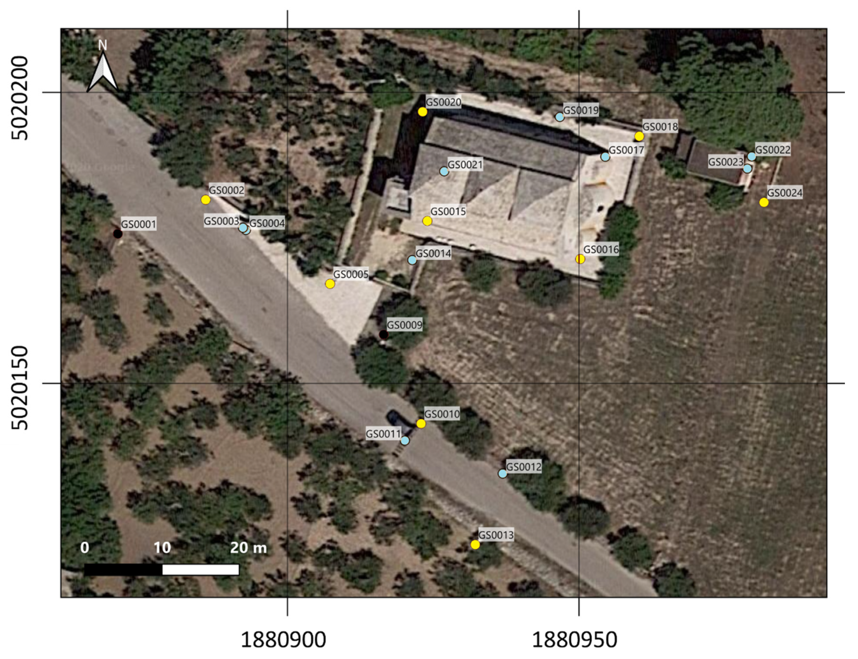
Figure 3.
Study area: All Saints’ Monastery of Cuti, located in the province of Bari (Southern Italy). The RGB orthophoto and the 3D scene representation produced by handling RPAS-photogrammetric data are reported on the left and on the right of the panel, respectively. Ground Control Points (GCPs) (in yellow) and Check Point (in light blue) locations are represented on the orthophoto. (Coordinate Reference System: WGS84/Pseudo-Mercator (EPSG:3857)).

Figure 4.
Volume density levels generated from RPAS-based and TLS-based point clouds are reported on the (top) and on the (bottom), respectively. This parameter was computed within a sphere with a radius equal to 0.05 m.
Figure 4.
Volume density levels generated from RPAS-based and TLS-based point clouds are reported on the (top) and on the (bottom), respectively. This parameter was computed within a sphere with a radius equal to 0.05 m.

Figure 5.
M3C2 distance and Distance Uncertainty are depicted at the (top) and at the (bottom), respectively. The unit measurement is the meter.
Figure 5.
M3C2 distance and Distance Uncertainty are depicted at the (top) and at the (bottom), respectively. The unit measurement is the meter.

Figure 6.
λ1, λ2 and λ3 estimated within a local sphere with a radius 0.05 m from RPAS-based (on the (top)) and TLS-based (on the (bottom)) point clouds, respectively.
Figure 6.
λ1, λ2 and λ3 estimated within a local sphere with a radius 0.05 m from RPAS-based (on the (top)) and TLS-based (on the (bottom)) point clouds, respectively.

Figure 7.
Histogram of λ1, λ2 and λ3 estimated within a local sphere with a radius 0.05 m from RPAS-based (on the (top)) and TLS-based (on the (bottom)) point clouds, respectively.
Figure 7.
Histogram of λ1, λ2 and λ3 estimated within a local sphere with a radius 0.05 m from RPAS-based (on the (top)) and TLS-based (on the (bottom)) point clouds, respectively.

Figure 8.
Histogram of eigenvalues-based geometric features extracted from the RPAS dense point cloud.
Figure 8.
Histogram of eigenvalues-based geometric features extracted from the RPAS dense point cloud.

Figure 9.
Histogram of eigenvalues-based geometric features extracted from the TLS dense point cloud.
Figure 9.
Histogram of eigenvalues-based geometric features extracted from the TLS dense point cloud.

Figure 10.
Anisotropy, planarity, linearity, mean curvature, eigenvalue sum, omnivariance extracted from RPAS.
Figure 10.
Anisotropy, planarity, linearity, mean curvature, eigenvalue sum, omnivariance extracted from RPAS.

Figure 11.
Anisotropy, planarity, linearity, mean curvature, eigenvalue sum, omnivariance extracted from TLS.
Figure 11.
Anisotropy, planarity, linearity, mean curvature, eigenvalue sum, omnivariance extracted from TLS.

Figure 12.
The variance of geometric features computed from the RPAS (on the (left)) and TLS (on the (right)) models.
Figure 12.
The variance of geometric features computed from the RPAS (on the (left)) and TLS (on the (right)) models.


Table 1.
Main features of RPAS-based and TLS-based point clouds.
| RPAS | TLS | |
|---|---|---|
| ACQUISITION TIME (min) | ~14 | ~150 |
| PROCESSING TIME (min) | ~974 | ~300 |
| DENSE POINT CLOUDS NUMEROSITY (n° points) | 28,202,789 | 195,939,535 |
Table 2.
RMSE referring to the point cloud extracted using RPAS-photogrammetry for both GCPs and CPs. The total values and their components along the three axes (x, y, and z) are reported.
Table 2.
RMSE referring to the point cloud extracted using RPAS-photogrammetry for both GCPs and CPs. The total values and their components along the three axes (x, y, and z) are reported.
| GCPs | CPs | |
|---|---|---|
| RMSEx (m) | 0.014 | 0.009 |
| RMSEy (m) | 0.016 | 0.013 |
| RMSEz (m) | 0.026 | 0.022 |
Publisher’s Note: MDPI stays neutral with regard to jurisdictional claims in published maps and institutional affiliations. |
© 2021 by the author. Licensee MDPI, Basel, Switzerland. This article is an open access article distributed under the terms and conditions of the Creative Commons Attribution (CC BY) license (https://creativecommons.org/licenses/by/4.0/).
Share and Cite
MDPI and ACS Style
Capolupo, A. Accuracy Assessment of Cultural Heritage Models Extracting 3D Point Cloud Geometric Features with RPAS SfM-MVS and TLS Techniques. Drones 2021, 5, 145. https://0-doi-org.brum.beds.ac.uk/10.3390/drones5040145
AMA Style
Capolupo A. Accuracy Assessment of Cultural Heritage Models Extracting 3D Point Cloud Geometric Features with RPAS SfM-MVS and TLS Techniques. Drones. 2021; 5(4):145. https://0-doi-org.brum.beds.ac.uk/10.3390/drones5040145
Chicago/Turabian StyleCapolupo, Alessandra. 2021. "Accuracy Assessment of Cultural Heritage Models Extracting 3D Point Cloud Geometric Features with RPAS SfM-MVS and TLS Techniques" Drones 5, no. 4: 145. https://0-doi-org.brum.beds.ac.uk/10.3390/drones5040145