
UAV-Based Landfill Land Cover Mapping: Optimizing Data Acquisition and Open-Source Processing Protocols


1
Remote Sensing and Geodata Unit, Institut Scientifique de Service Public (ISSeP), 4000 Liège, Belgium
2
ANAGEO, Université Libre de Bruxelles (ULB), 1050 Brussels, Belgium
*
Author to whom correspondence should be addressed.
Drones 2022, 6(5), 123; https://0-doi-org.brum.beds.ac.uk/10.3390/drones6050123
Submission received: 23 March 2022
/
Revised: 4 May 2022
/
Accepted: 5 May 2022
/
Published: 9 May 2022
(This article belongs to the Topic Remote Sensing and Geoinformatics in Agriculture and Environment)
Abstract
:Earth observation technologies offer non-intrusive solutions for monitoring complex and risky sites, such as landfills. In particular, unmanned aerial vehicles (UAVs) offer the ability to acquire data at very high spatial resolution, with full control of the temporality required for the desired application. The versatility of UAVs, both in terms of flight characteristics and on-board sensors, makes it possible to generate relevant geodata for a wide range of landfill monitoring activities. This study aims to propose a robust tool and to provide data acquisition guidelines for the land cover mapping of complex sites using UAV multispectral imagery. For this purpose, the transferability of a state-of-the-art object-based image analysis open-source processing chain was assessed and its sensitivity to the segmentation approach, textural and contextual information, spectral and spatial resolution was tested over the landfill site of Hallembaye (Wallonia, Belgium). This study proposes a consistent open-source processing chain for the land cover mapping using UAV data with accuracies of at least 85%. It shows that low-cost red-green-blue standard sensors are sufficient to reach such accuracies and that spatial resolution of up to 10 cm can be adopted with limited impact on the performance of the processing chain. This study also results in the creation of a new operational service for the monitoring of the active landfill sites of Wallonia.
Keywords:
landfill management; land cover; UAV; multispectral; GRASS; machine learning; OBIA; supervised classification1. Introduction
The volume of waste produced by human activity, and in particular by the construction and industrial sectors, is constantly increasing, with a volume exceeding 67 million tons of waste per year in Belgium [1]. The management, treatment, and recycling of these different types of waste is therefore a challenge for health, the environment, and the economy. Although the number of waste recycling channels is increasing, notably due to the prospects offered by enhanced landfill mining [2], the burial of waste in landfills is historically the primary solution and continues to be so for a series of specific wastes, which cannot be directly recycled or are considered hazardous. To reduce environmental impact, secure routine operation, and monitor compliance with imposed standards, landfill managers are subject to various obligations: control pollution levels (soil, air, and water, including biogas emission and odor nuisance, limit leachate leakage and diffuse pollution of waste due to light fractions spreading by wind, etc.), avoid mechanical instabilities (maximum slope angles), and control the landfill completion rate and the volumes of waste buried. For all these controls, ground survey solutions exist but are hampered by the complexity, danger, and size of the areas to be monitored.
Earth observation (EO), from satellite to Unmanned Aerial Vehicles (UAVs), is a proven technology for many of these control activities. The last decade has seen UAV technology adopt one of the most dynamic growth patterns in the aerospace sector [3]. The increasing payload and autonomy capabilities of UAVs contribute to the diversification of business applications, technology, and operations research. The miniaturization of EO sensors and the optimization and automation of data processing chains reinforce this observation. UAVs can be equipped with a growing range of single-band, multispectral or hyperspectral sensors operating in the visible, infrared, or microwave spectrums [4]. The cost benefits of UAVs for fine-scale environmental monitoring as an alternate to satellite or airborne platform systems is established as they are more flexible, mission specific, and versatile [5]. This is particularly true when the research focuses on a concise area (<1 km²) with a need for ultra-high resolution (sub-decimeter resolution) and/or with full control of the flight conditions (weather, cloud-free, revisit time, or acquisition properties such as viewing angle, height, path, etc.). In addition, offering the possibility of non-intrusive data collection, UAVs are particularly appropriate for the monitoring of complex sites with a high degree of risk (ground operation, dangerous terrain, etc.). Such case studies include the monitoring of engineering structures [6], construction sites [7], brownfields [8], quarries [9], agriculture fields [10], and forestry plots [11]. By verifying all these criteria, active landfills are particularly relevant study sites.
In their review about the use of drone technology in municipal solid waste management and landfilling, Sliuzar et al. [12] noted that the most mature field of application of drones on waste disposal sites is the analysis of its spatial properties. The photogrammetric pre-processing algorithms are efficient and allow for obtaining qualitatively comparable results to ground-based approaches (global navigation satellite system (GNSS) solutions) with a non-negligible saving of resources and reduction in risks. The second most studied field of application is the field of thermal and gas surveys to detect surface emissions or leaks in the biogas collection network. Despite suitable hardware design, this task remains difficult because of the spatial and temporal variability of emissions and the high dynamics of the air environment. Sliuzar et al. [12] highlighted that in addition to the effective spatial characterization of landfills by UAV data, the overall management of the site and the reduction in environmental impacts would benefit from new developments aiming at the automatic-type recognition of land cover (LC) features. The authors noted that machine learning (ML) and waste recognition algorithms are improving at a rapid pace [13], with new promising application from deep learning (DL) algorithms [14,15]. The review listed only one paper applying ML specifically to landfills for LC features extraction [16], but noted that the technological evolution of these techniques should lead to more publications in the near future.
Regarding the use of ML and DL techniques in the specific fields of waste management, Xia et al. [17] demonstrated their use and their relevance at all stages, from the generation of municipal solid waste to their recycling or landfilling. This review noted the growth of ML and DL publications in recent years with the prevalence of artificial neural networks (ANNs), DL such as convolutional neural networks (CNNs), support vector machine (SVM), support vector regression (SVR), and random forest (RF) methods. The authors listed only one publication applying ML to EO data: ANNs applied to thermal data for assessing and predicting landfill surface temperature [18]. This highlights once again the novelty of the use of EO data, including UAV, for the monitoring of landfill and specifically for LC features extraction.
Extracting automatically wall-to-wall LC maps from ultra-high-resolution data is indeed challenging [19]. Active landfills’ LC is usually very fragmented and LC change can be highly dynamic. It continuously evolves because of new deposits, earthworks, natural growth of vegetation, and rehabilitation activities. As such, automated classification methods are needed. When dealing with very high-resolution data, numerous studies conclude that object-based image analysis (OBIA) supervised classification is the most suited technique for LC mapping compared with pixel-based approaches [20,21]. OBIA approaches have the advantages of considering shape and texture properties in addition to spectral properties. Wyard et al. [16] successfully transposed the OBIA processing chain developed by Grippa et al. [22] to UAV data for the automatic LC classification of the Hallembaye landfill site (Wallonia, Belgium) reaching an overall accuracy (OA) of 80.5%. This open-source processing chain includes tools for unsupervised segmentation, its optimization, and multiple ML classification algorithms. Its original design is for city-scale to regional LC mapping using very high-resolution satellite data [22,23]. Beaumont et al. [24] and Bassine et al. [25] applied it to the classification of aerial orthophotos combined with normalized digital surface models (nDSMs). To our knowledge, this processing chain has only been applied twice to UAV data in addition to the work of Wyard et al. [16]. Wijesingha et al. [26] performed a binary classification of the invasive plant species Lupinus polyphyllus within grasslands from a red-green-blue (RGB) camera; Souffer et al. [27] classified visible and thermal UAV imagery for the automatic extraction of photovoltaic panels, obtaining an F-factor of 98.7%.
As a continuation of the work of Wyard et al. [16], this study has two objectives. Given the complexity of landfills and the high revisit rate desired in such application, the first objective is to provide guidelines on the necessary UAV flight characteristics (spatial and spectral resolution) required for the automatic multi-class LC mapping of such site. The second objective is to provide a robust and optimized open-source OBIA processing chain as automated as possible for the production of LC maps using UAVs data. The robustness of the processing chain presented in Wyard et al. [16] was first assessed by applying it to new datasets acquired over the same landfill site (Hallembaye, Belgium). The sensitivity of the results to segmentation approach, textural information, spectral resolution, spatial resolution, and contextual information were then assessed. It was indeed suggested that a better spectral resolution can improve class discrimination and that the segmentation approach as well as contextual information can also help to refine the results [16]. It was demonstrated that textural information has a significant positive impact on UAV image classification results [28]. In addition, the spatial resolution on the ground is crucial because it affects the objects that can be discriminated depending on their size, the UAV flight height and speed, and thus directly the area that can be covered and the amount of data to process.
Section 2 describes the characteristics of the Hallembaye landfills as well as the UAVs datasets acquired on this site. The description of the OBIA LC processing chain can also be found in Section 2. Section 3 starts by a presentation of the results for six series of experiments: robustness, sensitivity to segmentation approach, sensitivity to textural information, sensitivity to spectral resolution, sensitivity to spatial resolution, and sensitivity to contextual approach. Section 3 ends with an analysis of feature contribution from the best results. The results are discussed in Section 4 while the conclusions and prospects are presented in Section 5.
2. Materials and Methods
2.1. Study Area
This research focuses on the landfill site of Hallembaye, located in the east of Wallonia (Belgium) less than 2 km from the Dutch border, on the Communes of Oupeye and Visé (Figure 1). The site covers an area of 31.4 ha. It has been operating since 1989 for the burial of household waste, non-hazardous and non-toxic industrial waste, inert waste, as well as residual waste from sorting centers. The landfill is characterized by areas in exploitation (active) and areas under temporary rehabilitation (passive), with a wide variety of LC objects. The Hallembaye landfill site is part of the dozen-site network in Wallonia submitted to the same exploitation and obligation protocols.
2.2. Data
Three UAV datasets were used in this study (Table 1). The two main datasets used in this study were acquired on 1 March 2021, using two vectors and two different sensors. The DJI®® Mavic 2 Enterprise has a three-band true-color on-board sensor by default (Dataset #1) [29]. The MicaSense®® RedEdge MX Dual Camera System embarked on the Mavic M600 Pro UAV provides spectral information in 10 wavelengths (Dataset #2) [30]. The RedEdge MX provides blue (center wavelength: 475 nm (bandwidth: 32 nm)), green (560 (27)), red (668 (14)), red-edge (717 (12)), and near-infrared (NIR) channels (842 (57)). The RedEdge MX Blue provides aerosol (444 (28)), green (431 (14)), red (650 (16)), and red-edge channels (705 (10) and 740 (18)).
To a lesser extent the classification results of a third dataset acquired on 3 October 2019 were exploited (Dataset #0; [16]). Its acquisition was performed using the DJI®® Mavic M600 Pro hexacopter equipped with a DJI® Zenmuse X5 [31]. This camera captures RGB information. For all three datasets, frontal and side overlap was set between 70 and 80% while camera angle was set to 70°. All flights were conducted from the top of the landfill for visibility reasons. In order to achieve the objectives of spatial resolution (between 3 and 4 cm) and overlap, the height above ground level (AGL) of 90 m (Datasets #0 and #1) and 45 m (#2) were defined in relation to the take-off point. As a result, and in view of the battery capacities, the following areas could be covered: 27.6 ha for Dataset #0, 56.1 ha for Dataset #1 and 15.2 ha for Dataset #2 (Figure 1).
The flight planner for Dataset #0 was Pix4DCapture [32], while DJI Ground Station pro ([33] was used for planning Datasets #1 and #2. Ground control points ((GCPs) 9 for Dataset #0 and 6 for Datasets #1 and #2) were used to improve the geometric accuracy of the photogrammetric processing. These GCPs were acquired using a Sokkia GRX1 global navigation satellite system (GNNS) receiver [34], which is compatible with the real time kinematic (RTK) technique and operates the permanent network of Walcors stations [35]. The accuracies in XYZ given by the device are lower than 1 cm. Images were radiometrically corrected and mosaicked using the Pix4D Mapper software v4.4.12. RGB orthomosaics and digital surface models (DSMs) were obtained for Datasets #0 and #1. The spatial resolution of the orthomosaics ranges between 2.8 and 3.8 cm. From Dataset #2, a 10-band orthomosaic characterized by a 3.2 cm spatial resolution was obtained.
This study mainly used Datasets #1 and #2 as input for sensitivity experiments on the OBIA processing chain described in the following sections (Section 2.3 and Section 2.4). To perform an objective comparison of the classification results, Dataset #1 was clipped to the extent of Dataset #2. This smaller area comprises a wide range of LC classes and includes active waste deposit areas. The classification results obtained from Dataset #0 in a previous work [16] were exploited for comparison with results obtained with the new classification results generated in this study from Dataset #1 and Dataset #2.
2.3. OBIA Processing Chain
The OBIA processing chain used to extract the LC of Hallembaye was based on the work of Wyard et al. [16]. They transposed and modified the open-source processing chain developed by Grippa et al. [22] to UAVs data. This processing chain was based on an integration of GRASS GIS and R within a Python programming environment. The code was implemented in a Jupyter Notebook. The modifications applied to the original work of Grippa et al. [18] included textural index calculation and implementation of feature selection through the classification optimizer presented by Georganos et al. [36]. The full flowchart of the processing chain can be found in the study by Grippa et al. [22].
2.3.1. Classification Scheme and Sampling
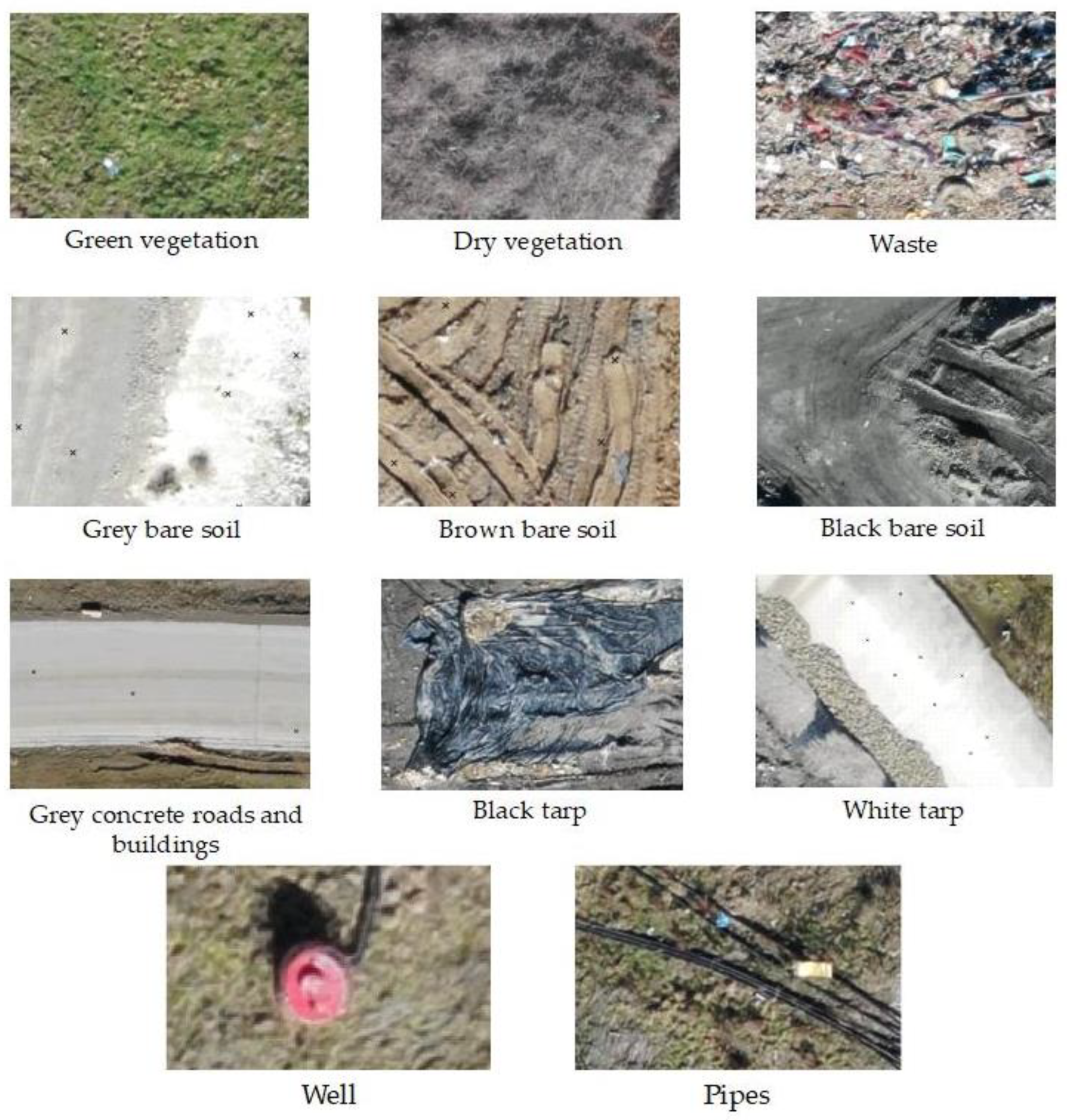
The variability in spatial coverages and LC change over time impact classification scheme and sampling strategy. A total of 11 classes were identified over the common dataset coverage (Figure 2).
These are green and dry vegetation, grey concrete roads and buildings, mostly spread over the passive area and surroundings of the site. Waste, black tarps, white tarps and three types of soils (embankments, classified according to their colors) are visible in the active area. These classes correspond to the LC generally observed on active landfills in Wallonia and other neighboring regions. However, the nature of the soil embankments may vary from one landfill to another, as well as the typology of the buried waste. This variation can also be observed over time, due to the strong dynamics of these sites. Wells and pipes are specific elements that are not included in our automatic classification tests. The site manager maintains geolocation files of these objects which allowed us to extract both classes from the UAV images. UAV data are valuable for updating these objects by manual digitalization. Samples were collected for the 9 remaining classes. A random stratified sampling was used to obtain a minimum of 100 points per class. Sample classes were identified through a visual interpretation. A total of 70 training points per class were considered for the training, the remaining samples were considered for the validation (Table 2).
2.3.2. Image Segmentation
The extraction of objects from raster data can be performed using various GRASS-GIS add-ons and strategies. For instance, the i.segment GRASS GIS add-on, which is based on a region-growing algorithm [37], can be applied to raster data. Object recognition is tuned by setting a segment minimum size and a ‘threshold’ representing the spectral similarity between adjacent segments. A threshold of 0 allows only identical valued pixels to be merged, while a threshold of 1 allows everything to be merged. The i.superpixels.slic (Simple Linear Iterative Clustering (SLIC)) GRASS-GIS add-on is another option. It creates superpixels using a k-means method, based on the work of Radhakrishna et al. [38]. This add-on divides the image into a number of compact and nearly uniform superpixels.
2.3.3. Object Statistics Computation/Feature Creation
For each segment, a wide range of statistics can be computed from the various raster provided as input. The available raster statistics are: minimum, maximum, range, mean, mean of absolute values, standard deviation, sum, sum of absolute values, variance, coefficient of variation, first quartile, median, third quartile, and percentile 90 statistics. Input raster can be optical bands, DSM and its by-products, and textural indexes computed from optical bands. The r.texture GRASS GIS add-on was implemented after the studies by Haralick et al. [39,40] and allows the computation of a few dozen texture indexes including angular second moment (ASM), contrast (CONTR), correlation (CORR), entropy (ENTR), difference variance (DV), inverse difference moment (IDM), sum average (SA), and sum entropy (SE). Raster statistics can be completed with the morphological attributes of the segments, namely: area, perimeter, compact circle, compact square, fractal dimension (fd), x coordinates (xcoords), and y coordinates (ycoords).
2.3.4. Classification
The classification stage was performed using v.class.mlR in GRASS GIS [41]. Classification performance is optimized through feature selection using the RF classifier [36]. Indeed, RF was shown to be highly accurate and stable with high-dimensional data which is the case in this study given the large variety of features that can be created (Section 2.3.3) [42].
2.3.5. Post-Processing
The resulting map was scanned by a convolutional square window of 7 × 7 pixels. The class value of the central pixel was replaced by the most frequently occurring class value in the neighborhood (modal filter). The size of the neighborhood was chosen by considering a minimum mapping unit (MMU) of 20 cm (image spatial resolution x neighborhood size = MMU). This operation was performed using the r.neighbors GRASS GIS add-on.
2.4. Experiments
To reach the objectives of this study, sensitivity experiments were carried out on Dataset #1 and Dataset #2 (Section 2.2). Table 3 summarizes the tests performed and their main characteristics.
First, the robustness of the processing chain was assessed by applying it without modification to the new RGB Dataset (#1) in its native spatial resolution (3.8 cm), which was set with similar acquisition characteristics as Dataset #0 used by Wyard et al. [16]. Related tests are Test #0 and Test #1.
Second, the sensitivity of the processing chain to the segmentation approach was assessed. More precisely, two approaches were tested. On the one hand, a region-growing approach was applied. Objects were extracted from the multispectral data (either 3 or 10 bands) in their native spatial resolution by directly applying the i.segment GRASS GIS add-on. This first approach used the original version of the processing chain [16]. Then, a hybrid clustering approach was performed. A preliminary step of superpixel creation was performed using the i.superpixels.slic GRASS-GIS add-on and used as objects seeds for subsequent region growing with i.segment. The division of the image into a number of compact and nearly uniform superpixels provided useful clustering cues to guide image segmentation and accelerated the convergence of the region-growing algorithm (i.segment), which was then applied. Crommelinck et al. [43] tested the SLIC approach for the segmentation of 5 cm UAV data and concluded that “the approach is not suitable as a standalone approach for object delineation. However, it shows high potential for a combination with further methods”. The SLIC approach can indeed be used in combination with other algorithms or as a first step in image segmentation [44,45,46,47]. Such approach is noted to be more efficient than the region-growing approach especially from a computation time point of view (less time than traditional method). Wu et al. [46] combined the SLIC superpixel to the region-growing algorithm with satisfying results. For both approaches, parameters were determined by human eye assessment. Tests related to this experiment are Test #1 and Test #2.
Third, the sensitivity of the processing chain results to the textural information was assessed. In fact, textural information was proven to have a significant positive impact on UAV image classification results [28]. This was confirmed by Wyard et al. [16], who improved the classification OA by 10% by using eight textural indexed computed from a single pseudo-panchromatic band and by performing a feature selection. In this study, two approaches were tested to determine which one provided the best results for reasonable computation time. Texture computation is indeed very time-consuming (in our case, 1 h per textural index depending on the resources available). The first approach used a pseudo-panchromatic band (pseudo_panchro = 0.2989 × R + 0.5870 × G + 0.1140 × B) and the calculation of eight textural indexes on the latter (hereafter referred to the texture from one panchromatic band approach). The second approach consisted of the calculation of a variable number (3, 5, and 8) of textural indexes on the raw spectral bands (hereafter referred to the texture by spectral band approach). For both approaches a window of 15 pixels was set by experimentation. Tests were carried out on RGB Dataset #1 and 10-band Dataset #2 in their native spatial resolution using the best segmentation approach identified in the previous experiment. Tests related to this experiment are Test #1 (best result of previous experiment), Test #3, Test #4, Test #5, Test #6, Test #7, Test #8, and Test #9.
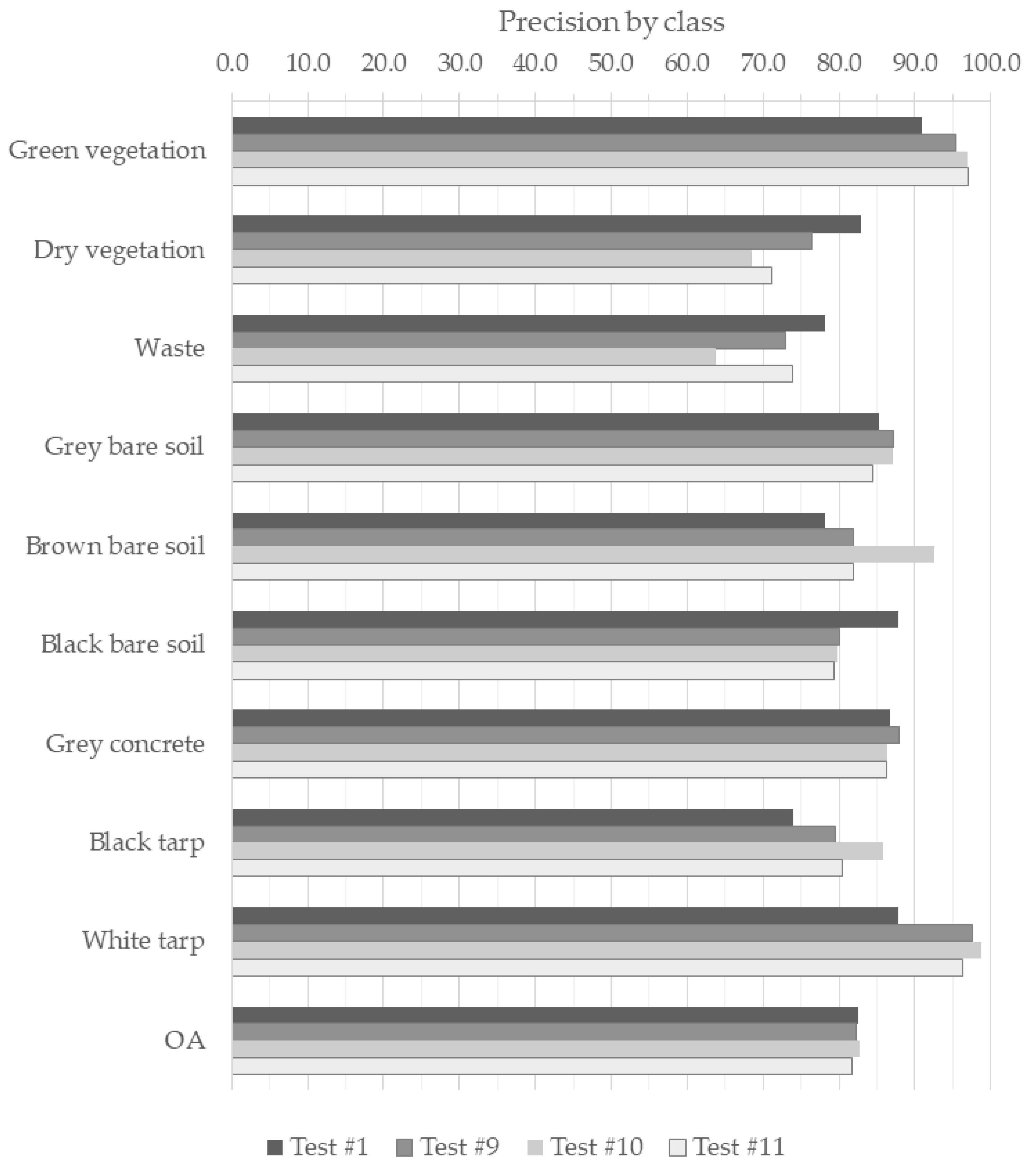
Fourth, the sensitivity of the processing chain to spectral resolution was assessed. The hypothesis was indeed raised that a better spectral resolution can improve class discrimination [16]. Results obtained for the three-band Dataset #1 were compared with results obtained for the 10-band Dataset #2 using the best texture combination identified in the previous experiment. The focus was on the precision by class. Tests used for this analysis are Test #1 (best result of previous experiment using the RGB dataset), #Test 9 (best result of previous experiment using the 10-band dataset), Test #10, and Test #11.
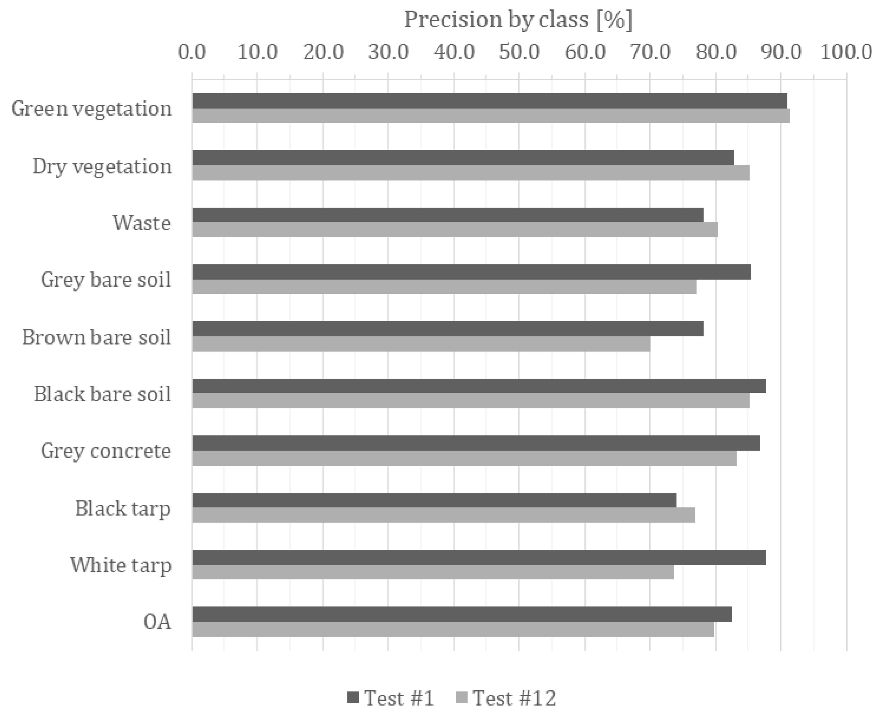
Fifth, the sensitivity of the processing chain to spatial resolution was assessed. The spatial resolution on the ground is crucial because it impacts the objects that can be discriminated depending on their size, the UAV flight height and speed, and thus directly the area that can be covered and the amount of data to process. For this purpose, Dataset #1 was resampled from its native resolution of 3.8 cm to 10 cm and the best configuration of the processing chain determined by the previous experiments was adapted to this coarser resolution. Namely, parameters were adapted to keep the same order of size. The result was then compared with the best results obtained from the processing chain using Dataset #1 in its native spatial resolution. The related tests are Test #1 (best result of previous experiment) and Test #12.
Sixth, the sensitivity of the processing chain to contextual information was evaluated. For this propose, Dataset #1 was used in its original spatial resolution, and xcoords and ycoords were added as features. The related test is Test #13. Results were then compared with the same test performed without contextual information (Test #1).
Tests #1 to #12 were performed using the same features. These features consist of the following raster statistics: min, max, range, mean, stddev, sum, variance, first_quart, median, third_quart; and the following geometric attributes: area, perimeter, compact_circle, fd. Test #13 used all these features, plus xcoords and ycoords in the geometric attributes.
3. Results
Table 3 provides an overview of results obtained during the sensitivity experiments that are described in Section 2.4. The OA of the different tests exhibits a 10% variation, from 78.8% to 88.5%, which is significant given the complexity of the task (a nine-class supervised classification) and the high OA which are already achieved. The following subsections analyze the results in detail by sensitivity experiment.
3.1. Robustness
Results confirm the robustness of the OBIA processing chain for the LC mapping of a landfill site using drone data. By applying this processing chain to a new RGB dataset (Test #1) and compared with Wyard et al. [16] (Test #0), results show close OA of 80.5% (Test #0) and 82.6% (Test #1) (Table 3). Test #1 OA is also significantly better than Test #0. It can therefore be concluded that the processing chain is robust and applicable to RGB UAV images taken at different dates. The only constraint is that the sampling must be checked from one dataset acquisition to another.
3.2. Sensitivity to Segmentation Approach
Both tested segmentation approaches (see Section 2.4. for details) provide consistent results but the direct application of i.segment remains the best compromise between computation time and performance. In fact, the results show that Test #1 has a significantly higher OA (82.6%) than Test #2 (76.7%) (Table 3). Figure 3 provides a visual comparison of both segmented images and classification results.
A significant drop in dry vegetation (−10.0%), brown bare soil (−8.4%), black bare soil (−9.5%), grey concrete (−10.2%), and white tarp (−11.0%) class precision explains the counter performance of Test #2 and is illustrated in Figure 3e. As expected, Test #2 allows for significantly reducing the segmentation computation time by 60% but requires two steps of manual parameter fitting instead of one for Test #1. The first segmentation approach is therefore considered the most relevant.
3.3. Sensitivity to Textural Information
Although the addition of textural information generally refines the classification results and influences the precision of certain classes, the new tested approaches do not outperform the original approach applied to RGB images by Wyard et al. [16]. However, the approach generating the best results varies following the spectral resolution of the dataset.
On the one hand, by comparing the texture by spectral band approaches (new approaches) performed on the RGB imagery (Dataset #1) (Test #3, Test #4, Test #5) to the texture from one panchromatic band approach (original approach) (Test #1), results show that the latter remains the best with OA peaking at 82.6% (Figure 4a). The OA of Tests #3, #4, and #5 are very close with values of 78.8, 79.8, and 80%, respectively (Figure 4a). Increasing the number of texture indexes allows for refining the classification results, especially when this number goes from three (Test #3) to five (Test #4) (+1%), which corresponds to the addition of DV and CORR. The addition of IDM, SE, and ENTR has a much more limited impact on classification results (Test #5). The addition of textural information generally benefits to all classes. By analyzing the precision by class, the texture by spectral band approach allows to refine the identification of green vegetation, dry vegetation, waste, and black tarp, which correspond to the most textured classes (Figure 2).
On the other hand, tests performed on the 10-band imagery (Dataset #2) show that contrary to the RGB imagery, texture by spectral band approaches are more indicative with OA peaking at 82.2% when eight textures per spectral band of the first RedEdge MX camera are used (Test #9) (Figure 4b). In fact, the use of a panchromatic band, and the calculation of textures on the latter produced OA of 80.0% (Test #6). On the contrary, the addition of up to eight textures calculated directly on the raw spectral bands contributes to the improvement of the OA. However, the texture from spectral band approach is very time consuming compared with the texture from one pseudo-panchromatic band approach, up to +900% in terms of processing time for a gain of about 2% in OA. As observed for the tests performed on the RGB imagery, the gain in OA is larger when the number goes from three (80.9%) to five (82.2%) than to five to eight (82.4%) (Test #7, #8, and #9 respectively).
3.4. Sensitivity to Spectral Resolution
The results show that an RGB sensor allows for obtaining more comparable results than the 10-band sensor such as the RedEdge MX Dual Camera System although potential complementarities are identified. To reach this statement, several specific tests were carried out on the 10-band imagery (Dataset #2).
Classification results using either or both MX cameras together show limited changes in OA. Maximum OA (82.8%) was achieved using only the RedEdge MX Blue camera, offering two RedEdge bands (Test #10) (Figure 5).
Comparative analysis by class shows that the first MX camera (having one band in the RedEdge and one in the NIR) improves the classification of the dry vegetation and the waste matrix by about 10% compared with the MX Blue sensor (Test #9). In contrast, the MX Blue sensor improves the discrimination of grey bare soil and black membranes (Test #10). This may highlight the value of using the two sensors in separate classifications and crossing the results in post processing. Indeed, combining the 10 bands in the classification chain tends to average out these improvements, and results in a lower OA (81.2%) (Test #11).
In the end, the OA of the best results obtained from the 10-band imagery (i.e., the RedEdge MX Blue camera classification using eight textures, Test #10) is comparable to the best results obtained from the RGB imagery (i.e., three bands RGB, panchromatic band, eight textures, Test #1) with OA of 82.8% and 82.6%, respectively. It can therefore be concluded that for this LC mapping scheme applied to the Hallembaye landfill, an RGB sensor is sufficient. However, it should be noted that the addition of spectral information offered by the MX Dual camera contributes to improve the classification of brown bare soils by more than 14%, black tarp by almost 12%, white tarp by 11%, and green vegetation by 6%. On the other hand, the RGB classification performs better for dry vegetation and waste (more than 14% better for these two classes) and for black bare soils (by 8%). In total, the overall OA is not significantly different between these two tests, but potential complementarities are identified.
3.5. Sensitivity to Spatial Resolution
Tests performed on the RGB imagery (Dataset #1) show that a spatial resolution of 10 cm is sufficient to obtain OA of about 80%. The comparison between Test #1 (3.8 cm) and Test #12 (10 cm) shows rather close OA (Figure 6). However, Test #1 remains significantly better (+2.8%). Regarding precision by class, the 10 cm resolution seems to be more suitable only for the identification of dry vegetation (+2.4%), waste (+2.2%), and black tarp (+2.9%), which are classes rather heterogeneous. Indeed, the 10 cm resolution allows generalizing information for these classes.
In addition, the use of a coarser resolution has several advantages: reduction in the UAV flight duration, reduction in the number of images to be pre-processed and consequently the general processing time, possibility to cover a larger area. For a 10 cm resolution, compared with a 3.8 cm resolution, the flight duration is reduced by 72% while the number of images is reduced by 90%.
3.6. Sensitivity to Contextual Information
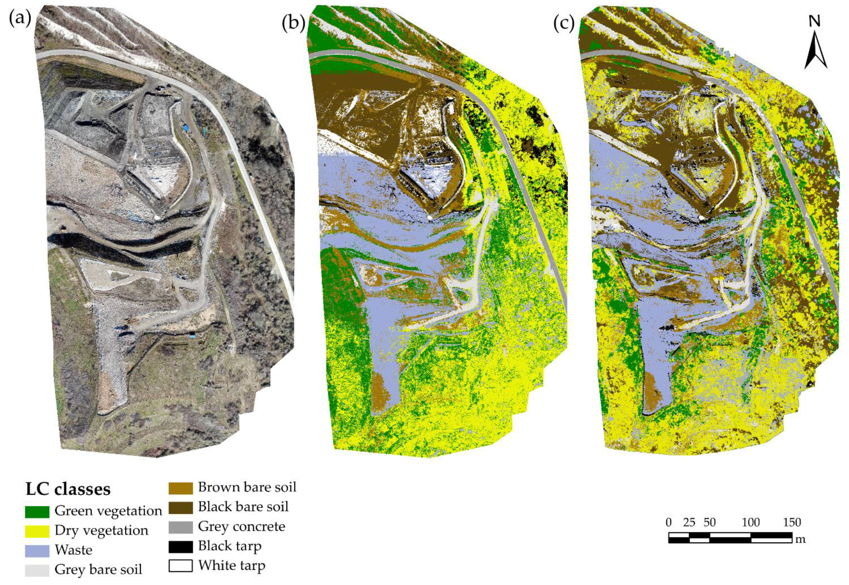
The addition of contextual information, namely, the x and y coordinates of the objects in their features, produces the most significant improvement of classification with OA of 88.5%. Compared with Test #1, this is an improvement of nearly +6%. Almost all classes benefit from the additional contextual information with gain in precision by class ranging from +4.6% (green vegetation) to +20% (black tarp). Two classes show a drop in their precision: grey concrete (−10.2%) and white tarp (−13.4%). The analysis of the Test #13 confusion matrix reveals a strong confusion between these two classes leading to precision by class of 76.6% and 74.4%, respectively. Grey concrete and white tarp have indeed close optical characteristics; however, this is their spatial proximity and their marginal distribution over the site at this acquisition date which explains their confusion (Table 4). Regarding the seven remaining classes, confusion is very limited so that their precision is above 85% (five classes with precision above 90%). In addition, the comparison between the classified LC map obtained from Test #13 (Figure 7b) and the original image (Figure 7a) reveals unwanted classification artefacts of white tarp, black tarp, and grey bare soil. These classes are characterized by a reduced and marginal distribution at this acquisition date which results in clustering in the sampling as well. The x and y coordinates used as features results in the artifacts observed in Figure 7b and in confusion between classes of similar appearance which are spatially close to each other.
3.7. Features Contribution
Among all tests performed, Test #13 produced the best OA with a value of 88.5%. Regarding precision by class, Test #13 performs better with seven classes above 85% (five above 90%) and a minimum precision by class of 74.4% (Table 4). Such performance is achieved using a total of 22 features. Contextual information explains 70.7% of this performance, while features related to optical bands and texture indexes account for 16.9% and 12.4%, respectively.
By analyzing the second-best test (Test #10) when contextual information is not used, the resulted classified LC map does not exhibit artefacts as strong as Test #13 (Figure 7c). As a reminder, Test #10 used the five-band RedEdge MX Blue camera, slope, and eight textures computed for each spectral band, which allows reaching OA of 82.8%. This performance is achieved using a larger number of features: 94 in total. Features related to texture indexes explain 70.4% of this performance, while features related to optical bands and to slope account for 26.0% and 3.6%, respectively.
Finally, it should be noted that the classification of shadows is a challenge as illustrated in both classified LC map presented in Figure 7.
4. Discussion
The final results show that the OBIA processing chain allows for producing consistent LC classifications for at least two dates using RGB UAV imagery. They also show that low-cost RGB standard sensors are sufficient to reach accuracies above 85% and that spatial resolution of up to 10 cm can be adopted with limited impact on the performance of the processing chain. The sensitivity experiments carried out on the segmentation approach, textural, and contextual information, and spectral and spatial resolution show that when contextual information is not taken into account, OA peaks at 82.8%. Dry vegetation, waste and black bare soil are the classes which systematically drag down the classification performance with precision below 80% and even below 70% for dry vegetation and waste. Confusions originate from similar color and texture. The addition of NIR and red edge spectral bands obviously fails to solve color-related confusion. The addition of contextual information, namely the x and y coordinates of objects, allows to significantly improve the performance of the processing chain with a +6% jump in OA reaching 88.6%. However, unwanted classification artifacts are observed in the resulted LC map due to a reduced and marginal distribution of certain class at this acquisition. The following subsections discuss these results in view of the original objectives of the study, of improvements that are still possible in the processing chain, and in the prospects offered by this work for the monitoring of landfill sites.
4.1. Robustness and Replicability of the Processing Chain
The first objective of this study was to provide a robust and optimized open-source OBIA processing chain as automated as possible for the production of LC maps using UAVs data. The satisfying OA obtained for two UAV data acquisition dates demonstrates the replicability of the processing chain. This replicability was already demonstrated in the processing of airborne and satellite data at very high spatial resolution [22,24,25]. It was demonstrated for the processing of UAV data.
However, the large number of activities carried out on an operational landfill does not allow for a fully automated processing chain: the selection of training and validation points must be checked manually between each dataset. However, experience shows that most of the changes are made in the active zone, thus limiting the number of points to be updated (max 1 to 2 h for the update of more than 1000 sampled points). Given the temporal variability of landfill waste and soil deposits in terms of color, the automation of this selection, such as in the works of Radoux et al. [48] or using active learning strategies [49], appears complex on such site, but can be more easily considered in other applications.
In this study, the replicability of the processing chain was demonstrated for at least two different seasons: early autumn and late winter. On the one hand, the flight conducted in early October 2019 (early autumn) occurred at the end of the growing season. The advantages are: (a) less confusion between vegetation and other LC classes as vegetation is mostly green; (b) and shadows can be limited. On the other hand, the flights conducted in early March 2021 (late winter) occurred outside the growing season. This has two advantages: (a) the mapping of the ground cover is partly free of vegetation and therefore it is possible to better discriminate objects on the ground; (b) and it is carried out in the cold period that is favorable for the thermographic analysis of the site for the detection of biogas leaks, and therefore for the coupling of UAV-based services. The resulting difficulty is less discrimination of vegetated areas and consequently greater confusion between vegetation and other LC. For the other periods of year which have not yet been tested, late autumn and early spring can be more challenging. Indeed, the various states of the vegetation at these periods would add complexity to the discrimination of vegetation classes against soil classes and waste.
The LC context of the Hallembaye landfill is characteristic of the context of other Walloon landfills included in the monitoring network. We are therefore convinced, and the prospects include running this service routinely on all sites, of the replicability of the OBIA processing chain. However, it is crucial to adapt the sampling and classification strategy to the classes present on each site. Indeed, the legal provisions vary from one site to another, notably in the typology of the waste buried and in the status of the site (in activity, in post-management, or in rehabilitation). Depending on the local soil properties of the site, it is highly likely that the types of soil embankments will also vary from one site to another.
4.2. Data Acquisition Guidelines
The second objective of this paper was to provide guidelines on the necessary UAV flight characteristics required for the automatic multi-class LC mapping of dynamic sites. At the end of the empirical approach, we can conclude that the use of light UAV equipment with a traditional multispectral sensor with three visible bands appears to be the best compromise in terms of classification quality, flight autonomy, and consequently, the area that can be covered during a flight campaign. The current legislation on flight authorization (Regulation (EU) 2019/947 and Regulation (EU) 2019/945) is also more flexible for this type of equipment, compared with that applicable to M600 Pro such as UAVs.
The richer multispectral information shows limited improvement in the classification results in our case study. This observation is only valid for the equipment we compared and should be put into perspective with the opportunities offered by a UAV-borne spectrometer or those operating in other wavelength ranges [50,51].
In terms of recommendations for the flight height and the temporality of the acquisitions (frequency and period in the year), we feel it is necessary to relate this application to the other services using UAVs useful for landfill management. In this sense, our study shows that a spatial resolution of 10 cm is sufficient for the purpose of LC mapping. However, such a resolution complicates the photo-interpretation purposes as developed by Filkin et al. [52]. In this sense, we recommend aiming for a spatial resolution of less than or equal to 5 cm, allowing the photo-interpretation of all the features of interest present on a landfill.
The robustness of the processing chain was demonstrated in and out of the vegetation period for two acquisition dates (early autumn and late winter) with satisfying results in terms of OA. In terms of temporality, we recommend adjusting the acquisition frequency to the needs of the topographic monitoring of landfills that can use the same equipment, but keeping in mind that some periods of the year may be more challenging for LC mapping, as detailed in Section 4.1. More generally we recommend acquiring UAV data in weather and illumination conditions as homogeneous as possible.
4.3. Improving Classification Performances
Given the complexity of this classification (nine classes) and the high OAs that were achieved (88.5%), every percentage that can still be gained is significant but the task is difficult. The more classes and the higher the OA, the more difficult it is to further improve the OA. Sensitivity experiments performed on segmentation approach, textural, spatial, and textural information showed limited impact on the classification performances compared with the original version of the processing chain [16]. Still, the next step can be to take a closer look at the spectral signatures of the different types of waste and landfill to better guide the choice for specific sensor with a relevant spectral band. However, it should be noted that such a task is difficult because each site is different and hosts different wastes. Moreover, the availability of the relevant sensor on the market is not guaranteed.
The improvement of the classification performance can come from the addition of contextual features and/or of contextual post-processing rules [53]. Regarding the addition of contextual features, the addition of object location criteria (namely their x and y coordinates) in the features strongly impacted the classification results with a +6% jump in the OA reaching 88.6% (Test #13, see Section 3.6). However, unwanted classification artefacts were observed in the classified LC maps due to the clustering in the sampling of certain classes (Figure 7b). This clustering results from the reduced and marginal spatial distribution of certain classes such as black and white tarps. This situation can however change from one acquisition date to another as landfill sites rapidly change from day to day. In addition, this situation can also be solved with the extension of the study area. Indeed, the use of light UAV equipment allows for acquiring data over larger areas as explained in Section 4.1. Regarding the contextual post-processing rules, such rules must be adapted from one classification result to another. It is not compatible with our processing chain, which we want to be as automated as possible and replicable for other dates and for other sites.
The analysis of the classified LC maps (Figure 7) showed that the presence of shadows and classification is a challenge (Section 3.7). Several options are possible to tackle this problem. Image acquisition can be carefully planned to limit the presence of shadows (e.g., cloudy weather conditions avoid direct radiation and therefore shadows, around noon under sunny conditions). Another option is the addition of a shadow class to the classification scheme and its reclassification in post-processing using rules for instance. For the latter option, the use of slope and their orientation (also called “aspect”) can be relevant. However, as already noted, post-classification rules are not fully compatible with the first objective of this study.
Reaching OA above 90% would allow obtaining results of the same order as authors using other approaches for the LC mapping from UAV imagery. In fact, although OBIA combined to supervised classification is the most commonly used technique for LC mapping, other approaches also have their proof. OBIA combined with a fuzzy unordered rule induction algorithm outperforms decision tree and SVM with OA of 91.23% for a nine-class LC mapping over palm tree exploitation [53].
Another way of improvement to investigate in the near future is the use of deep-learning approaches [54]. However, creating fully labeled patches for semantic segmentation is dramatically time consuming and should be avoided as much as possible. A hybrid approach consisting of using state-of-the-art models such as Xception or DenseNet pre-trained on ImageNet dataset and using them as feature extractors to generate features to feed a conventional machine learning classifier such as random forest, is an option to investigate [55,56].
4.4. Integration of the Method into Landfill Control Actions
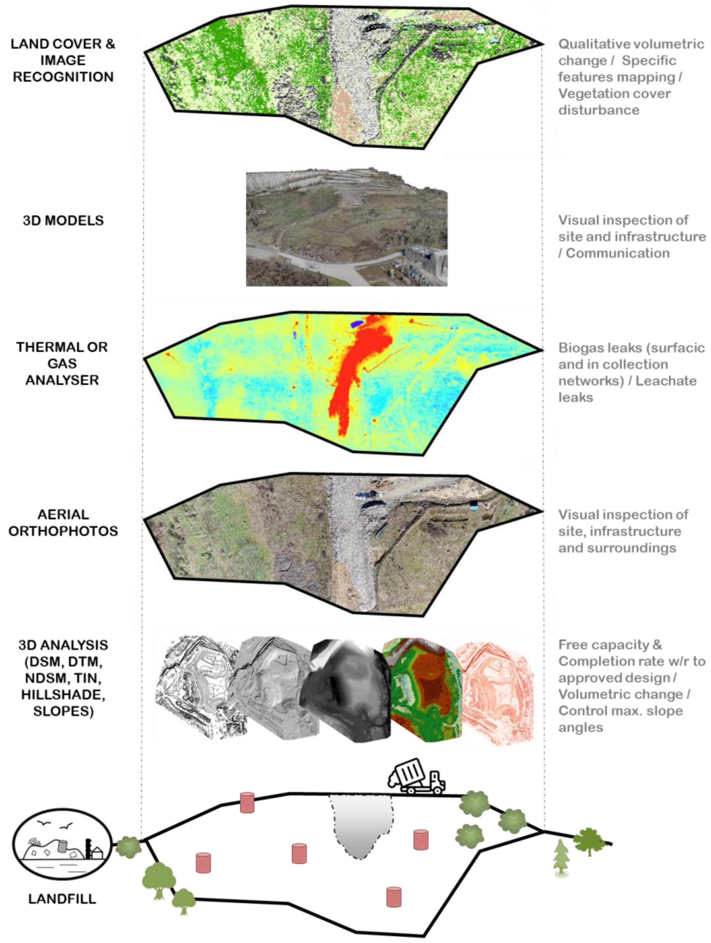
During the last decade, the qualitative improvement of sensors, vectors, and processing make UAVs an efficient technology for the identification and evaluation of environmental effects and the regular analysis of operations related to landfill management [12]. Beyond the services currently considered as operational, such as the extraction of information on the spatial properties of a landfill [57] or its thematic inspection in connection with technological monitoring and operational control [50], this study adds a new LC mapping service in the framework of our landfill control actions (Figure 8).
Achieving OA below 90% does not preclude the value of this application. Indeed, the managers in the temporal follow-up of the deposits are particularly interested in the study of the volumetric changes on site. For this application, the qualitative contribution (what type of waste, soils, vegetation growth, etc.) is value-added data. The generalization of the classification in “super object”, delimiting a waste mass or an excavated zone, namely allows for bringing this qualification to the volumetric statistics.
The proposed methodology not only offers a solution for the qualification and quantification of LC features over landfills, it also can contribute to a better mapping of illegal dumping sites (discriminating waste deposits from surrounding features), to the monitoring of other complex sites (construction site, quarries, etc.), or for other applications where only UAVs can provide suitable resolutions.
5. Conclusions
Achieving the qualitative standards of classification is a challenge and a difficulty on sites as complex and in constant evolution as a landfill. This study aimed to develop a robust and automated tool and to provide data acquisition guidelines for LC mapping of such complex sites using UAV multispectral imagery. For this purpose, the robustness of the object-based supervised classification processing chain originally developed by Grippa et al. [22] and adapted to UAV data by Wyard et al. [16] was assessed. Its sensitivity to the segmentation approach, textural information, spectral resolution, spatial resolution, and contextual information were also tested. The experimental design included the use of three distinct UAV datasets acquired using two vectors and three sensors at two acquisition dates over the Hallembaye landfill.
The sensitivity experiments performed on the OBIA processing chain demonstrates the added value of the use of contextual information as features in addition to features computed from optical and texture index rasters with a gain in OA of +6% reaching 88.5%. In fact, when contextual properties are not taken into account, OA peaks at 82.8% and confusions remain between classes of similar spectra and texture.
Regarding the first objective of this study (production of a robust and automated tool), the results proved the replicability of the OBIA processing chain for at least two acquisition dates (early autumn and late winter). The processing chain developed in this study may be used for other acquisition dates although the rapid evolution and different aspects of the vegetation during early spring and late autumn can add a challenge to the discrimination of LC classes. The processing chain can be used over other sites with the condition of adapting the classification schema to the LC classes observed over these sites.
Regarding the second objective of this study (the formulation of acquisition guidelines), the use of low cost and light UAV equipment with a standard RGB sensor appears to be the best compromise in terms of classification quality, flight autonomy, and consequently, the area that can be covered during a flight campaign. Results show that spatial resolution of up to 10 cm can be adopted with limited impact on the performance of the processing chain.
Among all the options considered to further improve the classification performance, the use of DL techniques is particularly promising and should certainly be investigated.
Finally, this study results in the creation of a new operational service for the monitoring of active landfill sites of Wallonia.
Author Contributions
Conceptualization, C.W. and B.B.; Data curation, C.W. and B.B.; Funding acquisition, B.B.; Investigation, C.W.; Methodology, C.W., B.B. and T.G.; Project administration, B.B. and E.H.; Resources, E.H.; Software, C.W.; Supervision, B.B. and T.G.; Validation, C.W.; Writing—original draft, C.W. and B.B.; Writing—review and editing, T.G. and E.H. All authors have read and agreed to the published version of the manuscript.
Funding
This research was conducted in the framework of the “CETEO” project (https://www.issep.be/wp-content/uploads/Projet-CETEO.pdf; accessed on 23 March 2022), which was funded by the internal Moerman fund of Institut Scientifique de Service Public (ISSeP).
Institutional Review Board Statement
Not applicable.
Informed Consent Statement
Not applicable.
Data Availability Statement
Data and a Jupyter Notebook containing the processing chain are available on GitHub: https://github.com/cwyard/Drones_paper_ressources (accessed on 20 March 2022).
Acknowledgments
The authors acknowledge ISSeP for funding this research. They would like to thank Julien Dumont and Fabian Stassen for performing the UAV flights and data acquisition, the Hallembaye landfill site managers for their interest and for opening the site to UAV flights, and Emilie Navette for her expertise of the site. The authors greatly thank the reviewers for their relevant comments which helped to improve this manuscript.
Conflicts of Interest
The authors declare no conflict of interest.
References
- Statbel, 2018. Available online: https://statbel.fgov.be/fr/themes/environnement/dechets-et-pollution/production-de-dechets (accessed on 12 December 2021).
- De Rijdt, A.; Neculau, C.; Wille, E. The rawfill concept: An integrated methodology and toolbox for selecting and launching enhanced landfill mining (elfm) projects. In Proceedings of the 4th International Symposium On Enhanced Landfill Mining, Mechelen, Belgium, 5–7 February 2018. [Google Scholar]
- Battsengel, G.; Geetha, S.; Jeon, J. Analysis of Technological Trends and Technological Portfolio of Unmanned Aerial Vehicle. J. Open Innov. Technol. Mark. Complex. 2020, 6, 48. [Google Scholar] [CrossRef]
- Chen, S.; Laefer, D.; Mangina, E. State of Technology Review of Civilian UAVs. Recent Pat. Eng. 2016, 10, 160–174. [Google Scholar] [CrossRef] [Green Version]
- Majid, M.I.; Chen, Y.; Mahfooz, O.; Ahmed, W. UAV-Based Smart Environmental Monitoring. In Employing Recent Technologies for Improved Digital Governance; Information Science Reference: Hershey, PA, USA, 2020. [Google Scholar] [CrossRef]
- Shafiee, M.; Zhou, Z.; Mei, L.; Dinmohammadi, F.; Karama, J.; Flynn, D. Unmanned Aerial Drones for Inspection of Offshore Wind Turbines: A Mission-Critical Failure Analysis. Robotics 2021, 10, 26. [Google Scholar] [CrossRef]
- Tkáč, M.; Mésároš, P. Utilizing drone technology in the civil engineering. Sel. Sci. Pap. J. Civ. Eng. 2019, 14, 27–37. [Google Scholar] [CrossRef] [Green Version]
- Štroner, M.; Urban, R.; Seidl, J.; Reindl, T.; Brouček, J. Photogrammetry Using UAV-Mounted GNSS RTK: Georeferencing Strategies without GCPs. Remote Sens. 2021, 13, 1336. [Google Scholar] [CrossRef]
- Nagendran, S.; Mohamad, I.; Mohd, A. Application of UAV photogrammetry for quarry monitoring. War. Geologi. 2020, 46. [Google Scholar] [CrossRef]
- Kim, J.; Kim, S.; Ju, C.; Son, H.I. Unmanned Aerial Vehicles in Agriculture: A Review of Perspective of Platform, Control, and Applications. IEEE Access 2019, 7, 105100–105115. [Google Scholar] [CrossRef]
- Michez, A.; Piégay, H.; Lisein, J.; Claessens, H.; Lejeune, P. Classification of riparian forest species and health condition using multi-temporal and hyperspatial imagery from unmanned aerial system. Environ. Monit Assess 2016, 188, 146. [Google Scholar] [CrossRef] [Green Version]
- Sliuzar, N.; Filkin, T.; Huber-Humer, M.; Ritzkowski, M. Drone technology in municipal solid waste management and landfilling: A comprehensive review. Waste Manag. 2022, 139, 1–16. [Google Scholar] [CrossRef]
- Gonçalves, G.; Andriolo, U.; Pinto, L.; Bessa, B. Mapping marine litter using UAS on a beach-dune: A multidisciplinary approach. Sci. Total Environ. 2022, 706, 135742. [Google Scholar] [CrossRef]
- Bak, S.H.; Hwang, D.H.; Kim, H.M.; Yoon, H.J. Detection and monitoring of beach litter using uav image and deep neural network. Int. Arch. Photogramm. Remote Sens. Spat. Inf. Sci. 2019, XLII-3/W8, 55–58. [Google Scholar] [CrossRef] [Green Version]
- Fallati, L.; Polidori, A.; Salvatore, C.; Saponari, L.; Savini, A.; Galli, P. Anthropogenic marine debris assessment with unmanned aerial vehicle imagery and deep learning: A case study along the beaches of the Republic of Maldives. Sci. Total Environ. 2019, 693, 133581. [Google Scholar] [CrossRef] [PubMed]
- Wyard, C.; Beaumont, B.; Grippa, T.; Georganos, S.; Hallot, E. UAVs for fine-scale Open-Source Landfill Mapping. In Proceedings of the IEEE International Geoscience and Remote Sensing Symposium IGARSS, Brussels, Belgium, 11–16 July 2021. [Google Scholar] [CrossRef]
- Xia, W.; Jiang, Y.; Chen, X.; Zhao, R. Application of machine learning algorithms in municipal solid waste management: A mini review. Waste Manag. Res. 2021, 40, 609–624. [Google Scholar] [CrossRef] [PubMed]
- Abu Qdais, H.; Shatnawi, N. Assessing and predicting landfill surface temperature using remote sensing and an artificial neural network. Int. J. Remote Sens. 2019, 40, 9556–9571. [Google Scholar] [CrossRef]
- Horning, N.; Fleishman, E.; Ersts, P.J.; Fogarty, F.A.; Wohlfeil Zillig, M. Mapping of land cover with open-source software and ultra-high-resolution imagery acquired with unmanned aerial vehicles. Remote Sens. Ecol. Conserv. 2020, 6, 487–497. [Google Scholar] [CrossRef] [Green Version]
- Sibaruddin, H.I.; Shafri, H.Z.M.; Pradhan, B.; Haron, N.A. Comparison of pixel-based and object-based image classification techniques in extracting information from UAV imagery data. IOP Conf. Ser. Earth Environ. Sci. 2018, 169, 012098. [Google Scholar] [CrossRef]
- De Giglio, M.; Greggio, N.; Goffo, F.; Merloni, N.; Dubbini, M.; Barbarella, M. Comparison of pixel-and object-based classification methods of unmanned aerial vehicle data applied to coastal dune vegetation communities: Casal borsetti case study. Remote Sens. 2019, 11, 1416. [Google Scholar] [CrossRef] [Green Version]
- Grippa, T.; Lennert, M.; Beaumont, B.; Vanhuysse, S.; Stephenne, N.; Wolff, E. An open-source semi-automated processing chain for urban object-based classification. Remote Sens. 2017, 9, 358. [Google Scholar] [CrossRef] [Green Version]
- Georganos, S.; Brousse, O.; Dujardin, S.; Linard, C.; Casey, D.; Milliones, M.; Parmentier, B.; Van Lipzig, N.P.; Demuzere, M.; Grippa, T.; et al. Modelling and mapping the intra-urban spatial distribution of Plasmodium falciparum parasite rate using very-high-resolution satellite derived indicators. Int. J. Health Geogr. 2020, 19, 38. [Google Scholar] [CrossRef]
- Beaumont, B.; Grippa, T.; Lennert, M.; Vanhuysse, S.; Stephenne, B.; Wolff, E. Toward an operational framework for fine-scale urban land-cover mapping in Wallonia using submeter remote sensing and ancillary vector data. J. Appl. Remote Sens. 2017, 11, 036011. [Google Scholar] [CrossRef] [Green Version]
- Bassine, C.; Radoux, J.; Beaumont, B.; Grippa, T.; Lennert, M.; Champagne, C.; De Vroey, M.; Martinet, A.; Bouchez, O.; Deffense, B.; et al. First 1-M resolution land cover map labeling the overlap in the 3rd dimension: The 2018 map of Wallonia. Data 2020, 5, 117. [Google Scholar] [CrossRef]
- Wijesingha, J.; Astor, T.; Schulze-Brüninghoff, D.; Wachendorf, M. Mapping Invasive Lupinus polyphyllus Lindl. in Semi-natural Grasslands Using Object-Based Image Analysis of UAV-borne Images. PFG 2020, 88, 391–406. [Google Scholar] [CrossRef]
- Souffer, I.; Sghiouar, M.; Sebari, I.; Zefri, Y.; Hajji, H.; Aniba, G. Automatic Extraction of Photovoltaic Panels from UAV Imagery with Object-Based Image Analysis and Machine Learning. In WITS 2020. Lecture Notes in Electrical Engineering; Bennani, S., Lakhrissi, Y., Khaissidi, G., Mansouri, A., Khamlichi, Y., Eds.; Springer: Singapore, 2022; Volume 745. [Google Scholar] [CrossRef]
- Kwak, G.H.; Park, N.W. Impact of texture information on crop classification with machine learning and UAV images. Appl. Sci. 2019, 9, 643. [Google Scholar] [CrossRef] [Green Version]
- DJI®® Mavic 2 Enterprise Specs. Available online: https://www.dji.com/mavic-2-enterprise/specs (accessed on 23 March 2022).
- RedEdge MX Dual Camera Imaging System by MicaSence. Available online: https://micasense.com/dual-camera-system/ (accessed on 23 March 2022).
- Zenmuse X5 Specs. Available online: https://www.dji.com/be/zenmuse-x5/info#specs (accessed on 23 March 2022).
- PIX4D. Available online: https://www.pix4d.com/ (accessed on 23 March 2022).
- DJI GS PRO. Available online: https://www.dji.com/be/ground-station-pro (accessed on 23 March 2022).
- GRX1 GNSS Receiver. Available online: https://eu.sokkia.com/sokkia-care-products/grx1-gnss-receiver (accessed on 23 March 2022).
- Portail Walcors. Available online: https://gnss.wallonie.be/walcors.html (accessed on 23 March 2022).
- Georganos, S.; Grippa, T.; Vanhuysse, S.; Lennert, M.; Shimoni, M.; Kalogirou, S.; Wolff, E. Less is more: Optimizing classification performance through feature selection in a very-high-resolution remote sensing object-based urban application. GIScience Remote Sens. 2018, 55, 221–242. [Google Scholar] [CrossRef]
- Momsen, E.; Metz, M.; GRASS Development Team. Addon i.segment. In Geographic Resources Analysis Support System (GRASS) Software, Version 7.8; Open Source Geospatial Foundation: Chicago, IL, USA, 2020. [Google Scholar]
- Radhakrishna, A.; Shaji, A.; Smith, K.; Lucchi, A.; Fua, P.; Susstrunk, S. SLIC Superpixels; Technical Report no. 149300; EPFL: Lausanne, Switzerland, 2010. [Google Scholar]
- Haralick, R.M.; Shanmugam, K.; Dinstein, I. Textural features for image classification. IEEE Trans. Syst. Man Cybern. 1973, 6, 610–621. [Google Scholar] [CrossRef] [Green Version]
- Haralick, R. Statistical and structural approaches to texture. Proc. IEEE 1979, 67, 786–804. [Google Scholar] [CrossRef]
- Lennert, M.; GRASS Development Team. Addon v.class.mlR. In Geographic Resources Analysis Support System (GRASS) Software, Version 7.8; Open Source Geospatial Foundation: Chicago, IL, USA, 2020. [Google Scholar]
- Li, M.; Ma, L.; Blaschke, T.; Cheng, L.; Tiede, D. A systematic comparison of different object-based classification techniques using high spatial resolution imagery in agricultural environments. Int. J. Appl. Earth Obs. Geoinf. 2016, 49, 87–98. [Google Scholar] [CrossRef]
- Crommelinck, S.; Bennett, R.; Gerke, M.; Koeva, M.N.; Yang, M.Y.; Vosselman, G. SLIC superpixels for object delineation from UAV data. In Proceedings of the ISPRS Annals of the Photogrammetry, Remote Sensing and Spatial Information Sciences: International Conference on Unmanned Aerial Vehicles in Geomatics (UAV-G 2017), Bonn, Germany, 4–7 September 2017; Volume 4. [Google Scholar] [CrossRef] [Green Version]
- Kishorjit Singh, N.; Johny Singh, N.; Kanan Kumar, W. Image classification using SLIC superpixel and FAAGKFCM image segmentation. IET Image Processing 2020, 14, 487–494. [Google Scholar] [CrossRef]
- Hsu, C.Y.; Ding, J.J. Efficient image segmentation algorithm using SLIC superpixels and boundary-focused region merging. In Proceedings of the 2013 9th International Conference on Information, Communications & Signal Processing, Tainan, Taiwan, 10–13 December 2013; pp. 1–5. [Google Scholar] [CrossRef]
- Wu, H.; Wu, Y.; Zhang, S.; Li, P.; Wen, Z. Cartoon image segmentation based on improved SLIC superpixels and adaptive region propagation merging. In Proceedings of the 2016 IEEE International Conference on Signal and Image Processing (ICSIP), Beijing, China, 13–15 August 2016; pp. 277–281. [Google Scholar] [CrossRef]
- Zhang, S.; You, Z.; Wu, X. Plant disease leaf image segmentation based on superpixel clustering and EM algorithm. Neural Comput. Appl. 2019, 31, 1225–1232. [Google Scholar] [CrossRef]
- Radoux, J.; Lamarche, C.; Van Bogaert, E.; Bontemps, S.; Brockmann, C.; Defourny, P. Automated Training Sample Extraction for Global Land Cover Mapping. Remote Sens. 2014, 6, 3965–3987. [Google Scholar] [CrossRef] [Green Version]
- Lu, Q.; Ma, Y.; Xia, G.-S. Active learning for training sample selection in remote sensing image classification using spatial information. Remote Sens. Lett. 2017, 8, 1210–1219. [Google Scholar] [CrossRef]
- Natesan, S.; Armenakis, C.; Benari, G.; Lee, R. Use of UAV-borne spectrometer for land cover classification. Drones 2018, 2, 16. [Google Scholar] [CrossRef] [Green Version]
- Adão, T.; Hruška, J.; Pádua, L.; Bessa, J.; Peres, E.; Morais, R.; Sousa, J.J. Hyperspectral imaging: A review on UAV-based sensors, data processing and applications for agriculture and forestry. Remote Sens. 2016, 9, 1110. [Google Scholar] [CrossRef] [Green Version]
- Filkin, T.; Sliusar, N.; Ritzkowski, M.; Huber-Humer, M. Unmanned Aerial Vehicles for Operational Monitoring of Landfills. Drones 2021, 5, 125. [Google Scholar] [CrossRef]
- Kalantar, B.; Mansor, S.B.; Sameen, M.I.; Pradhan, B.; Shafri, H.Z.M. Drone-based land-cover mapping using a fuzzy unordered rule induction algorithm integrated into object-based image analysis. Int. J. Remote Sens. 2017, 38, 2535–2556. [Google Scholar] [CrossRef]
- Osco, L.P.; Junior, J.M.; Ramos, A.P.M.; de Castro Jorge, L.A.; Fatholahi, S.N.; de Andrade Silva, J.; Matsubara, E.T.; Pistori, H.; Gonçalve, W.N.; Li, J. A review on deep learning in UAV remote sensing. Int. J. Appl. Earth Obs. Geoinf. 2021, 102, 102456. [Google Scholar] [CrossRef]
- Çayir, A.; Yenidoğan, I.; Dağ, H. Feature extraction based on deep learning for some traditional machine learning methods. In Proceedings of the 2018 3rd International Conference on Computer Science and Engineering (UBMK), Sarajevo, Bosnia, 20–23 September 2018; pp. 494–497. [Google Scholar] [CrossRef]
- Karim, Z.; van Zyl, T. Deep Learning and Transfer Learning applied to Sentinel-1 DInSAR and Sentinel-2 optical satellite imagery for change detection. In Proceedings of the 2020 International SAUPEC/RobMech/PRASA Conference, Cape Town, South Africa, 29–31 January 2020; pp. 1–7. [Google Scholar] [CrossRef]
- Incekara, A.; Delen, A.; Seker, D.; Goksel, C. Investigating the utility potential of low-cost unmanned aerial vehicles in the temporal monitoring of a landfill. ISPRS Int. J. Geo-Inf. 2019, 8, 22. [Google Scholar] [CrossRef] [Green Version]
Figure 1.
Location of the Hallembaye landfill and of the UAVs datasets.

Figure 2.
LC classes observed over the Hallembaye landfill site (images from Dataset #1).

Figure 3.
Comparison between (a) the original RGB image, (b,c) the segmented and (d,e) classified results from Test #1 (b,d), and Test #2 (c,e).
Figure 3.
Comparison between (a) the original RGB image, (b,c) the segmented and (d,e) classified results from Test #1 (b,d), and Test #2 (c,e).

Figure 4.
Evaluation of the impact of the texture information treatment on (a) the RGB image classification, and on (b) the 10-band image classification: precision by class and overall accuracy (OA).
Figure 4.
Evaluation of the impact of the texture information treatment on (a) the RGB image classification, and on (b) the 10-band image classification: precision by class and overall accuracy (OA).

Figure 5.
Evaluation of the impact of the spectral information on the classification results in terms of precision by class and overall accuracy (OA).
Figure 5.
Evaluation of the impact of the spectral information on the classification results in terms of precision by class and overall accuracy (OA).

Figure 6.
Evaluation of the impact of the spatial resolution on the classification results in terms of precision by class and overall accuracy (OA).
Figure 6.
Evaluation of the impact of the spatial resolution on the classification results in terms of precision by class and overall accuracy (OA).

Figure 7.
(a) Original image from Dataset #2, (b) the classified LC map from Test #13, and (c) the classified LC map from Test #10.
Figure 7.
(a) Original image from Dataset #2, (b) the classified LC map from Test #13, and (c) the classified LC map from Test #10.

Figure 8.
Products and services offered by UAVs for the monitoring of landfills.


Table 1.
UAVs datasets over the landfill of Hallembaye.
| # Dataset | Date | Vector-Sensor | Height AGL [m] | Frontal-Side Overlap [%] | Camera Angle [°] | Spatial Res. [cm] | Spectral Res. [nm] | Coverage [ha] | # Images | # Flights |
|---|---|---|---|---|---|---|---|---|---|---|
| 0 | 3 October 2019—11 h 53–12 h 36 | Mavic DJI M600 Pro—DJI Zenmuse X5 | 90 | 80–70 | 70 | 2.8 | Blue, green, and red | 27.6 | 710 | 2 |
| 1 | 1 March 2021—11 h 36–13 h 14 | DJI Mavic 2 Enterprise 00-14MV | 90 | 75–75 | 70 | 3.8 | Blue, green, and red | 56.1 | 954 | 4 |
| 2 | 1 March 2021—13 h 32–14 h 32 | Mavic DJI M600 Pro—Micasense RedEdge MX Dual Camera System | 45 | 75–75 | 70 | 3.2 | RedEdge MX: blue (center wavelength: 475 nm (bandwidth: 32 nm)), green (560 (27)), red (668 (14)), red-edge (717 (12)), and NIR channels (842 (57)). RedEdge MX Blue: aerosol (444 (28)), green (431 (14)), red (650 (16)), red-edge channels (705 (10), and 740 (18)). | 15.2 | 25,862 | 2 |
Table 2.
Classification scheme and size of the training and test sets.
| LC Class | Training Set Size | Test Set Size |
|---|---|---|
| Green vegetation | 70 | 33 |
| Dry vegetation | 70 | 30 |
| Waste | 70 | 54 |
| Grey bare soil | 70 | 32 |
| Brown bare soil | 70 | 58 |
| Black bare soil | 70 | 98 |
| Grey concrete roads and buildings | 70 | 25 |
| Black tarp | 70 | 54 |
| White tarp | 70 | 41 |
Table 3.
Overview of all sensitivity experiments performed in the framework of this study.
| Experiment | Test Id | # Dataset | Input Raster | Segmentation Type and Parameters | OA [%] | |||||
|---|---|---|---|---|---|---|---|---|---|---|
| Robustness | Segmentation | Texture | Spectral Info. | Spatial res. | Context Info | |||||
| X | 0 * | 0 | RGB + Slope + 8 texture indexes computed from a pseudo-panchromatic band * | i.segment, threshold = 0.06, minsize = 20 * | 80.5 * | |||||
| X | X | X | X | X | 1 | 1 | RGB + Slope + 8 texture indexes computed from a pseudo-panchromatic band * | i.segment, threshold = 0.06, minsize = 20 * | 82.6 | |
| X | 2 | 1 | Same as Test 1 | Superpixel + i.segment | 79.5 | |||||
| X | 3 | 1 | RGB + Slope + 3 texture indexes (ASM, CONTR, SA) computed for each spectral band | Same as Test 1 | 78.8 | |||||
| X | 4 | 1 | RGB + Slope + 5 texture indexes (ASM, CONTR, CORR, DV, SA) computed for each spectral band | Same as Test 1 | 79.8 | |||||
| X | 5 | 1 | RGB + Slope + 8 texture indexes computed for each spectral band | Same as Test 1 | 80.0 | |||||
| X | 6 | 2 | MX 10 Bands + Slope + 8 texture indexes computed from a pseudo-panchromatic band | Same as Test 1 | 80.0 | |||||
| X | 7 | 2 | MX 5 Bands + Slope + 3 texture indexes (ASM, CONTR, SA) computed for each spectral band | Same as Test 1 | 80.9 | |||||
| X | 8 | 2 | MX 5 Bands + Slope + 5 texture indexes (ASM, CONTR, CORR, DV, SA) computed for each spectral band | Same as Test 1 | 82.2 | |||||
| X | X | 9 | 2 | MX 5 Bands + Slope + 8 texture indexes computed for each spectral band | Same as Test 1 | 82.4 | ||||
| X | 10 | 2 | MX Blue 5 Bands + Slope + 8 texture indexes computed for each spectral band | Same as Test 1 | 82.8 | |||||
| X | 11 | 2 | MX 10 Bands + Slope + 8 texture indexes computed for each spectral band | Same as Test 1 | 81.2 | |||||
| X | 12 | 1 ** | Same as Test 1 | Same as Test 1 | 79.7 | |||||
| X | 13 *** | 1 | Same as Test 1 | Same as Test 1 | 88.5 | |||||
* Test 0 on Dataset #0 was originally presented in Wyard et al. [16]; ** resampled to 10 cm; *** used xcoords and ycoords in the geometric attributes.
Table 4.
Confusion matrix of Test #13. PA: producer accuracy; UA: user accuracy.
| Classification | ||||||||||||||
|---|---|---|---|---|---|---|---|---|---|---|---|---|---|---|
| 11 | 12 | 21 | 31 | 32 | 33 | 41 | 42 | 43 | SUM | PA [%] | Class Prec. [%] | |||
| Reference | Green vegetation | 11 | 32 | 0 | 0 | 0 | 0 | 1 | 0 | 0 | 0 | 33 | 97.0 | 95.5 |
| Dry vegetation | 12 | 0 | 28 | 0 | 0 | 2 | 0 | 0 | 0 | 0 | 30 | 93.3 | 91.8 | |
| Waste | 21 | 1 | 2 | 43 | 0 | 6 | 0 | 0 | 2 | 0 | 54 | 79.6 | 89.8 | |
| Grey bare soil | 31 | 0 | 0 | 0 | 31 | 0 | 0 | 1 | 0 | 0 | 32 | 96.9 | 91.5 | |
| Brown bare soil | 32 | 1 | 1 | 0 | 5 | 50 | 0 | 0 | 1 | 0 | 58 | 86.2 | 85.5 | |
| Black bare soil | 33 | 0 | 0 | 0 | 0 | 1 | 94 | 0 | 3 | 0 | 98 | 95.9 | 96.9 | |
| Grey concrete constructions | 41 | 0 | 0 | 0 | 0 | 0 | 0 | 25 | 0 | 0 | 25 | 100.0 | 76.6 | |
| Black tarp | 42 | 0 | 0 | 0 | 0 | 0 | 1 | 0 | 53 | 0 | 54 | 98.1 | 94.0 | |
| White tarp | 43 | 0 | 0 | 0 | 0 | 0 | 0 | 21 | 0 | 20 | 41 | 48.8 | 74.4 | |
| SUM | 34 | 31 | 43 | 36 | 59 | 96 | 47 | 59 | 20 | 425 | ||||
| UA [%] | 97.0 | 94.1 | 90.3 | 100.0 | 86.1 | 84.7 | 97.9 | 53.2 | 89.8 | 100.0 | OA = 88.5% | |||
Publisher’s Note: MDPI stays neutral with regard to jurisdictional claims in published maps and institutional affiliations. |
© 2022 by the authors. Licensee MDPI, Basel, Switzerland. This article is an open access article distributed under the terms and conditions of the Creative Commons Attribution (CC BY) license (https://creativecommons.org/licenses/by/4.0/).
Share and Cite
MDPI and ACS Style
Wyard, C.; Beaumont, B.; Grippa, T.; Hallot, E. UAV-Based Landfill Land Cover Mapping: Optimizing Data Acquisition and Open-Source Processing Protocols. Drones 2022, 6, 123. https://0-doi-org.brum.beds.ac.uk/10.3390/drones6050123
AMA Style
Wyard C, Beaumont B, Grippa T, Hallot E. UAV-Based Landfill Land Cover Mapping: Optimizing Data Acquisition and Open-Source Processing Protocols. Drones. 2022; 6(5):123. https://0-doi-org.brum.beds.ac.uk/10.3390/drones6050123
Chicago/Turabian StyleWyard, Coraline, Benjamin Beaumont, Taïs Grippa, and Eric Hallot. 2022. "UAV-Based Landfill Land Cover Mapping: Optimizing Data Acquisition and Open-Source Processing Protocols" Drones 6, no. 5: 123. https://0-doi-org.brum.beds.ac.uk/10.3390/drones6050123