
Modified Mayfly Algorithm for UAV Path Planning
by
 , , , , and
Xing Wang
1 ,
,
Jeng-Shyang Pan
1 ,
,
Qingyong Yang
1,
Lingping Kong
2,
Václav Snášel
2 and
Shu-Chuan Chu
1,*
1
College of Computer Science and Engineering, Shandong University of Science and Technology, Qingdao 266590, China
2
Faculty of Electrical Engineering and Computer Science, VŠB-Technical University of Ostrava, 70032 Ostrava, Czech Republic
*
Author to whom correspondence should be addressed.
Drones 2022, 6(5), 134; https://0-doi-org.brum.beds.ac.uk/10.3390/drones6050134
Submission received: 19 April 2022
/
Revised: 8 May 2022
/
Accepted: 18 May 2022
/
Published: 23 May 2022
(This article belongs to the Section Drone Design and Development)
Abstract
:The unmanned aerial vehicle (UAV) path planning problem is primarily concerned with avoiding collision with obstacles while determining the best flight path to the target position. This paper first establishes a cost function to transform the UAV route planning issue into an optimization issue that meets the UAV’s feasible path requirements and path safety constraints. Then, this paper introduces a modified Mayfly Algorithm (modMA), which employs an exponent decreasing inertia weight (EDIW) strategy, adaptive Cauchy mutation, and an enhanced crossover operator to effectively search the UAV configuration space and discover the path with the lowest overall cost. Finally, the proposed modMA is evaluated on 26 benchmark functions as well as the UAV route planning problem, and the results demonstrate that it outperforms the other compared algorithms.
1. Introduction
Unmanned aerial vehicles (UAV), as opposed to manned aircraft, refer to unmanned aircraft that can be controlled by remote radio control equipment or airborne computers. UAVs are less expensive and more flexible than manned aircraft, and they can reach difficult or dangerous places for humans to perform tasks. Therefore, UAVs have been widely used in civil and military fields. In the civil field, drones have played an important role in agricultural plant protection environment, aerial photography, express transportation, remote sensing of the oceans, and so on. In the military field, military drones can replace pilots in complex and dangerous missions such as intelligence gathering and reconnaissance surveillance. If the UAV is to complete the above tasks, one of the basic capabilities that the UAV must have is path planning capability [1].
The UAV path planning problem is to plan a collision-free path for the UAV from the starting point to the target point under the given flight conditions and flight environment. The planned path has the minimum cost and satisfies the relevant constraints. This problem can be simply described as an optimization problem with multiple constraints [2], so it is a challenge to traditional optimization strategies. There are already many mature solutions to this problem. In the direction of path planning based on graph search, Ref. [3] uses the A* algorithm for the UAV path planning problem with the goal of taking the least risk and consuming the least amount of fuel. Ref. [4] uses the D* Lite algorithm to plan an efficient path to the fire point for firefighting UAVs. In the direction of path planning based on sampling, Ref. [5] uses a hybrid algorithm combined with the artificial potential field method and the RRT-Connect algorithm for the path planning problem of UAV. Even though the techniques described above are relatively mature in mathematical theory, they are inefficient when working with discontinuous and non-derivative functions [6]. When tackling the UAV route planning problem with many restrictions [7], they are readily trapped into local optimum solutions.
The path planning issue has been demonstrated to be an NP-hard problem, and the problem complexity grows with problem size [8]. When solving NP-hard problems, heuristic algorithms can produce high-quality solutions and are simple to implement. As a result, some well-developed meta-heuristics with good performance have been proposed in recent years, such as the Cuckoo Search algorithm (CS) [9,10], Particle Swarm Optimization (PSO) [11,12,13], Genetic Algorithm (GA) [14,15], Artificial Bee Colony (ABC) algorithm [16,17], Differential Evolution (DE) algorithm [18,19], Grey Wolf Optimizer (GWO) [20,21], Ant Colony Optimization (ACO) algorithm [22,23], etc.
The Mayfly algorithm (MA) [24] is a recently suggested optimization method, which takes the flight and mating behavior of the mayfly as the model. Female and male mayflies make up the entire mayfly population. The movements of the male and female mayflies offer the MA the capacity to conduct local searches, and the procedure of developing offspring through mayfly mating gives the MA global search capability.
At present, research on MA is still relatively small. Inspired by the bare-bones PSO (BBPSO) [25], and then, Juan Zhao [26] proposed the bare-bones mayfly algorithm. The chaotic mayfly algorithm was suggested by Mohamed A. M. Shaheen [27], who used a logical chaotic map to initialize the mayfly population. This paper presented a modified Mayfly Algorithm (modMA), which includes the exponent decreasing inertia weight strategy, adaptive Cauchy mutation, and an enhanced crossover operator to analyze the path planning issue of UAV from the ground station to the destination, and it achieves good results.
Many works on improving two-dimensional paths using metaheuristics have been proposed to this point. Ref. [28] used the bat and cuckoo algorithm in path planning. Ref. [29] used the grey wolf optimizer to tackle the UAV route planning issue. Ref. [30] used a chaotic cuckoo search algorithm to optimize drone paths in two-dimensional (2D) space. Besides, many researchers used other meta-heuristic algorithms to study UAV path planning problems [31,32,33]. However, no one has proposed the use of MA to tackle UAV path planning in a 2D environment. Hence, this paper will use the modified Mayfly Algorithm (modMA) to study this problem. The following are the contributions to this paper.
- (1)
- It proposes an enhanced crossover operator based on the MA, which can improve MA’s exploration capability and convergence speed. Then it proposes a modified Mayfly Algorithm (modMA), which combines the EDIW strategy, adaptive Cauchy mutation, and the enhanced crossover operator to balance the MA’s processes of exploration and exploitation;
- (2)
- It introduces three versions of the modMA and compares their performance on six 100 and 300 dimension benchmark functions;
- (3)
- Compare the three versions of the modified MA with other algorithms (MA, PSO, GWO, BOA) on twenty-six 50 dimension benchmark functions, and analyze the results of the experiments;
- (4)
- Use the three versions of the modified MA for tackling the 2D path planning problem of agricultural UAV.
This paper is organized as follows: The standard MA, as well as the problem of UAV path planning, are briefly described in Section 2. Section 3 provides three optimization ideas for improving the MA. In Section 4, two experiments are planned to compare the MA’s enhanced performance using different optimization ideas and apply the three versions of the modified MA to the path planning problem of the agricultural UAV. Section 5 concludes.
2. Related Work
This section will provide a quick overview of the standard MA and the two-dimensional path planning problem of UAV.
2.1. Standard Mayfly Algorithm
The proposed MA’s fundamental concept is derived from the flight and mating behavior of mayflies. It combines the advantages of PSO [11], GA [14] and FA [34]. MA initially produces a mayfly population comprising males and females at random. The current velocity and position of the ith mayfly are two n-dimensional vectors, they are denoted as and , respectively. Each mayfly modifies its position depending on its individual best () position and the best () position found by the whole mayfly swarm thus far.
2.1.1. Male Mayfly Flight
Male mayflies cluster together, which suggests that their positions are updated based on social and personal experience. is defined as the present position of the ith male mayfly at iteration t. Assuming that is the current position of the ith mayfly at iteration t, the position can be updated by adding to a velocity . Thus the male mayfly’s position update formula is:
Consider those male mayflies are always performing nuptial dances not far from the water. The male mayfly’s velocity update formula is as follows:
where is the visibility coefficient, and are defined as the positive constants representing the attraction. is the best position obtained by the ith male mayfly in dimension j. and are the Euclidean distances between and and between and , respectively. The gravity coefficient is given by g, which can be a fixed number between 0 and 1, or it can be steadily lowered over iterations as in Equation (3).
where and respectively represent the smallest and largest weights. The present and the total number of iterations are given by and , respectively.
The personal best position at iteration is determined by Equation (4).
The best male mayflies keep performing up and down motions through different velocities. The velocities of these male mayflies are determined by Equation (5).
where the nuptial dance coefficient is given by d, and r means a random value in the range to 1.
2.1.2. Female Mayfly Flight
Female mayflies do not cluster together, however, they move towards male mayflies. is defined as the present position of the ith female mayfly at iteration t. The change of the ith female mayfly in position is calculated as:
In the MA, male and female mayflies with the same individual fitness ranking will attract each other, and the female mayfly’s position changes in response to the location of a male mayfly with the same ranking. The female mayfly’s velocity update formula is:
where and are respectively defined as the ith female mayfly’s velocity and position in dimension j at iteration t. and are defined as the attraction constant and the visibility coefficient, respectively. is the Euclidean distance between the ith female mayfly and the ith male mayfly, is a random walk coefficient which suggests that a female is not attracted to a male, and r means a random value in the range −1 to 1.
2.1.3. Mating Procedure
The mating is represented by the crossover operator which provides the global search capability for the MA. In the MA, male and female mayflies with the same individual fitness ranking will mate with each other to produce offspring mayflies. The mating operation of each pair of male and female mayflies produces two offspring, and the formula for the crossover operator is:
where L means a random value in the range 0 to 1. Moreover, and denote the parents. Initially, the offspring’s velocity is set to zero.
2.1.4. Mutate the Genes of Offspring
The mutation operator provides partial local search capability for MA. The chosen offspring can be updated by adding a random value to the variable throughout this process, so the offspring are changed to
where the standard deviation and the standard normal distribution are represented by and , respectively.
2.1.5. Reduction of Nuptial Dance and Random Walk
Although these operators provide the MA with powerful local search capability, d and must be gradually reduced. Both values can be updated over the iterations t using Equations (10) and (11), respectively.
where is a fixed number between 0 and 1.
As previously stated, Algorithm 1 depicts the MA’s pseudo-code.
| Algorithm 1 Pseudocode of MA. |
| Input: male and female population sizes, and ; maximum iterations, ; visibility coefficient, ; learning factors, and ; nuptial dance coefficient, d; random flight coefficient, ; objective function, Output: Optimal solution
|
2.2. UAV Path Planning Problem
UAV path planning aims to discover the best flight route for the UAV given a variety of complicated flying restrictions such as threat constraints and fuel limits [35]. The flying height of the drone might be constant along its flight path from the start point to the target point, so this paper only focuses on the UAV’s horizontal flying distance. The mathematical model for UAV path planning and the cost function used to evaluate the planned path are described as follows.
2.2.1. Mathematical Model for Uav Path Planning
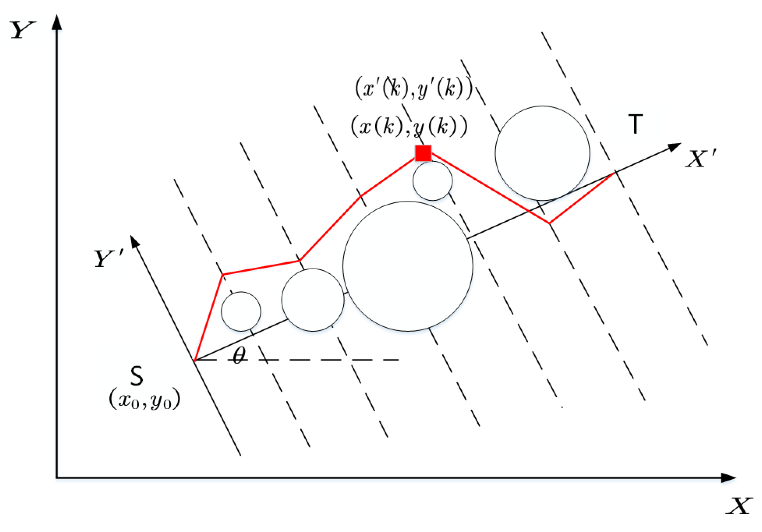
In this model, we define S and T to be the start point and target point of the UAV, respectively. It is crucial to prevent collisions with numerous obstacles during the flight of the drone. As a result, this paper employs circles of varying radii to substitute barriers of varying threat levels. So the task of a UAV flight is to find a flight path from S to T with the smallest overall cost while avoiding collisions with obstacles. Figure 1 depicts a schematic representation of the environment modeling for the UAV’s two-dimensional path planning. The path connected by the red line segments is the feasible path.
The segment between the S and T in the original coordinate system is split into equal portions by D vertical lines . We can get the path from S to T by picking a point on each vertical line. Thus, the planned path can be expressed as:
To accelerate the processing speed, let the segment be the horizontal axis and use Equation (13) to transfer each point in the to in the new coordinate system .
where denotes to the rotation angle of the , and the point is the coordinate in the .
As shown in Figure 1, the abscissa of each node in the can be calculated using formula , so the planned path can be simplified and expressed as:
2.2.2. Fitness Function Modeling
A fitness function can be used to calculate the cost of a planned path. The fitness function value can be used to judge the quality of the planned path. The fitness function established in this paper is defined as the sum of two cost functions, given as follows:
where denotes the total cost function of the planned path; denotes the cost of the planned path’s length; denotes the smoothness cost of the planned path. and are the weight coefficients of the above cost function, and they are defined as:
Given the UAV’s restricted energy supply, the shorter the planned path length, the less time and energy the UAV spends, and the better it is for the UAV. Assume that the topography of the flight environment and information on the threatened area are known. The start state and the target state are and , respectively. Hence, the cost related to the path length can be computed as:
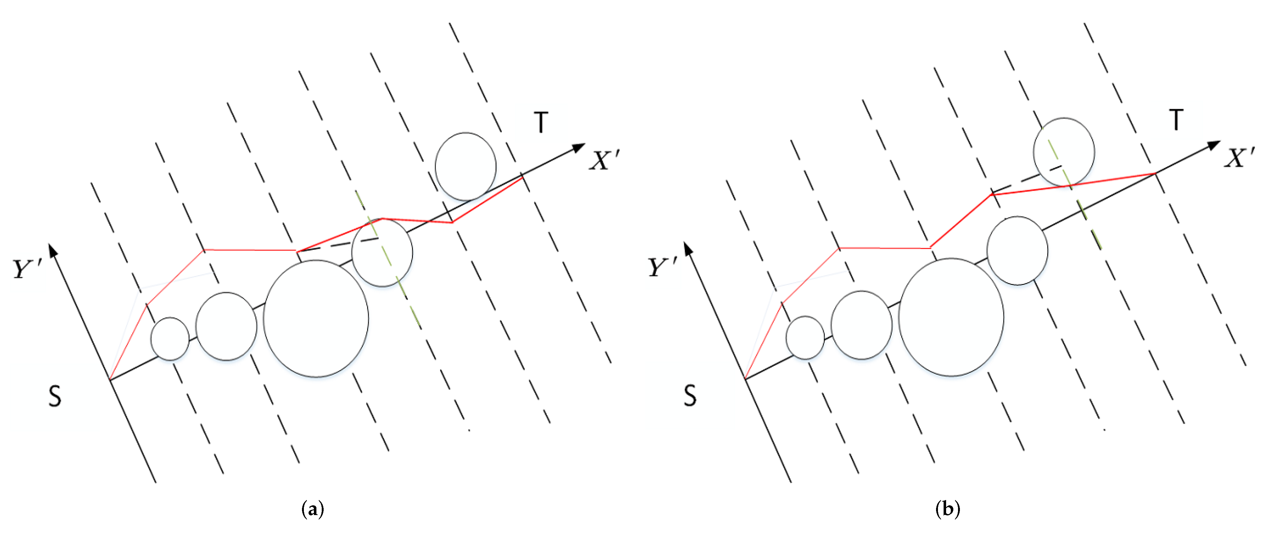
where is the distance between and . If the waypoint falls into the obstacle, we choose the intersection of the vertical line with the obstacle, the point closest to the waypoint, as the new search agent. Figure 2a,b depicts the post-collision processing flow. The path connected by the red line segments is the modified feasible path.
The smoothness cost evaluates the turning rate critical to generating feasible paths. The smooth cost can be computed as:
where the is the maximum turning angle, is the current turning angle, and is a vector representing the ith segment of the entire route.
3. Modifided Mayfly Algorithm
The standard MA has a better convergence speed than other swarm algorithms when dealing with low-dimensional situations. However, due to the influence of velocity fluctuation, the stability of the MA is poor, thus it leads to poor results. Furthermore, when dealing with high-dimensional nonlinear complicated situations, the MA cannot merely rely on its mechanism to get out of the local optimal zone, so the MA performs poorly on the multimodal functions. This section proposes a modified mayfly algorithm named modMA, which combines three strategies to improve the MA. One improvement is to use the exponent decreasing inertia weight strategy to improve MA, another uses the adaptive Cauchy mutation strategy to improve MA, and a third uses an enhanced crossover operator to improve MA.
3.1. Improvement 1: Exponent Decreasing Inertia Weight Strategy
There are many decreasing inertia weight strategies, such as linear [36], adaptive [37], logarithmic [38], and others [39]. The larger inertia weight in the earlier period is favorable to the exploration of particles, and the particles can search a larger space. The smaller inertia weight in the later period is beneficial to the exploitation of particles. This paper introduces the exponent decreasing inertia weight [40] into MA, formula is as follows:
where , , , and are the same to Equation (3).
3.2. Improvement 2: Adaptive Cauchy Mutaion Strategy
When utilizing Equations (1) and (2) in the standard MA to change the velocity of each male mayfly, the diversity of the entire mayfly population may decline. To mitigate this problem, the position of each male mayfly should be readjusted by using Cauchy-based mutation [41,42]. The standard Cauchy distribution’s probability density function can be described as:
where , the corresponding distribution function is expressed as:
Random numbers generated via the standard Cauchy distribution are shown below:
where denotes a random value produced by the inverse function of the standard Cauchy distribution function, means a random value in the range 0 to 1 produced by a uniform distribution.
According to Fogarty [43], improved performance is attained when the mutation rate falls exponentially with the number of iterations. Ref. [44] pointed out that the concept is related to that of the simulated annealing (SA) algorithm [45]. So after utilizing Equations (1) and (2) to change the position of each male mayfly, the position of each male mayfly needs to be readjusted using the Equation (22), which combines Cauchy mutation strategy with an adaptive mutation.
where is the ith individual calculated using Equations (1) and (2), and represents the mutated individual. is a contraction-expansion coefficient that controls the speed of convergence and it is defined as 0.15.
In this section, we combine the Cauchy mutation strategy with an adaptive mutation which can make the MA generate perturbations with a large step size in the early iterations so that the particles can jump from their current position to another and help MA escape the local optima. The perturbations with a smaller step size in the late iterations can speed up the convergence of the MA. It is worth mentioning that we do not use Cauchy-based mutation to readjust the positions of the particles calculated using Equations (1) and (5).
3.3. Improvement 3: Enhanced Crossover Operator
Although the crossover and reproduction operations of mayflies provide the MA with exploration ability as well as enhance the MA’s convergence speed, the MA has a not strong exploration ability. Hence, we use the horizontal crossover search [46] to improve it. The enhanced crossover operator of the MA employing horizontal crossover search is as follows:
where and are expansion coefficients, and they are both random values between −1 and 1 produced by a uniform distribution.
The horizontal crossover operation divides the problem-solving space of multi- dimensional into half-population of hypercubes, allowing new spots on the hypercube’s periphery to be sampled with a low probability, and reducing the blind region that are unable to explore by two paired parent individuals. Offspring generated using the horizontal crossover operation need to be compared with their parents, and individuals with greater fitness values are selected for the following iteration. It causes the MA to continuously converge to the best solution and ensure the convergence efficiency without affecting the optimization accuracy through the horizontal crossover operation.
We can also appropriately shrink or expand the search space generated by the two paired parent individuals. The formula of the crossover operator of the MA improved by shrinking the search space is as follows:
where and are the contraction coefficients, and they are both random values between 0.7 and 1 produced by a uniform distribution.
The formula of the crossover operator of the MA improved by expanding the search space is as follows:
where and are the expansion coefficients, and they are both random values between 1 and 1.3 produced by a uniform distribution.
Therefore, the enhanced crossover operator formula of MA can be described as:
where , , and are the random input numbers between [0, 1]. , , and are the switching probabilities, which control the method of offspring generation. For the value of switching probability , we refer to the parameter tuning technique of switching probability in the Butterfly Optimization Algorithm (BOA) [47]. From our simulations, we found that = 0.8, = 0.5, and = 0.5 work better for most applications.
4. Experimental Results and Application
In this part, we select a variety of numerical optimization functions from CEC benchmark functions to assess the effect of the modified MA presented in this article. Table A1 and Table A2 in Appendix A show the expression, dimension, domain of a variable, and minimum value of each benchmark function. These benchmark functions used in this study can be found in [48], and they are classified into two groups. The unimodal benchmark functions (F1–F14) and multimodal benchmark functions (F15–F26) are applied to calculate the abilities to exploit and explore of the algorithm benchmarked by benchmark functions, respectively.
To assess the efficacy of the three improvement techniques described in this study for MA, we first test and analyze the three versions of the improved MA through comparison experiment 1 by six benchmark functions from Table A1 and Table A2 with = 100 and = 300. It is worth mentioning that modMA-1 is characterized in this study as an MA that is improved by an adaptive Cauchy mutation strategy and the original crossover operator, modMA-2 is defined as an MA modified using only the enhanced crossover operator, and modMA is defined as an MA that incorporates three improved strategies.
To demonstrate that the proposed modMA outperforms other algorithms, we design the comparison experiment 2 for MA [24], modMA-1, modMA-2, modMA, PSO [11], GWO [20], and BOA [47] for 26 benchmark functions with = 50. Finally, we apply the three versions of the modified MA to the UAV path planning problem.
4.1. Parameter Settings of Seven Algorithms in Test
In the two experiments, we select MA [24], modMA-1, modMA-2, modMA, PSO [11], GWO [20], and BOA [47] for comparison. Table 1 shows the parameter settings of each algorithm. To promote equality in the comparison, all algorithms in this study are iterated 1000 times, the dimension is 50, and each algorithm has a maximum number of solutions of 40. For example, we use 20 female mayflies and 20 male mayflies for all simulations of MA. We analyze the Average (Avg) and Standard deviation (Std) of the fitness values after 30 runs on each benchmark function in both experiments.
4.2. Experiment 1: Comparison with MA, modMA-1, modMA-2,
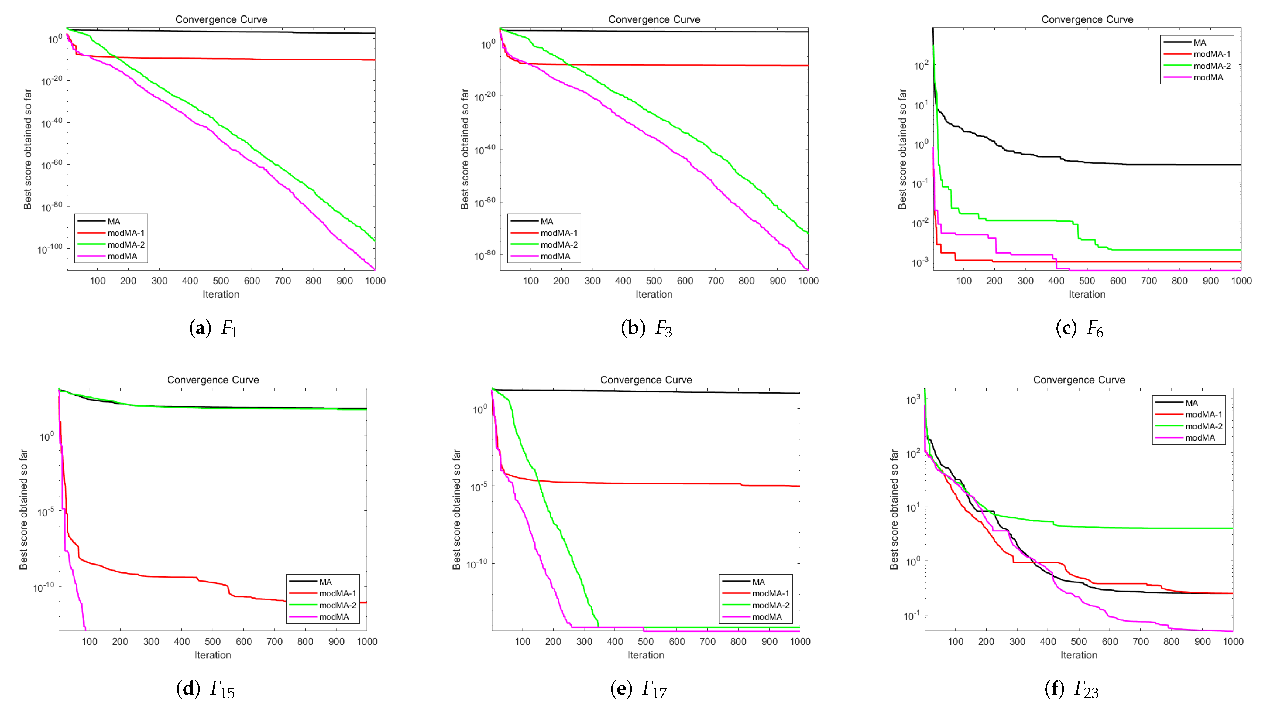
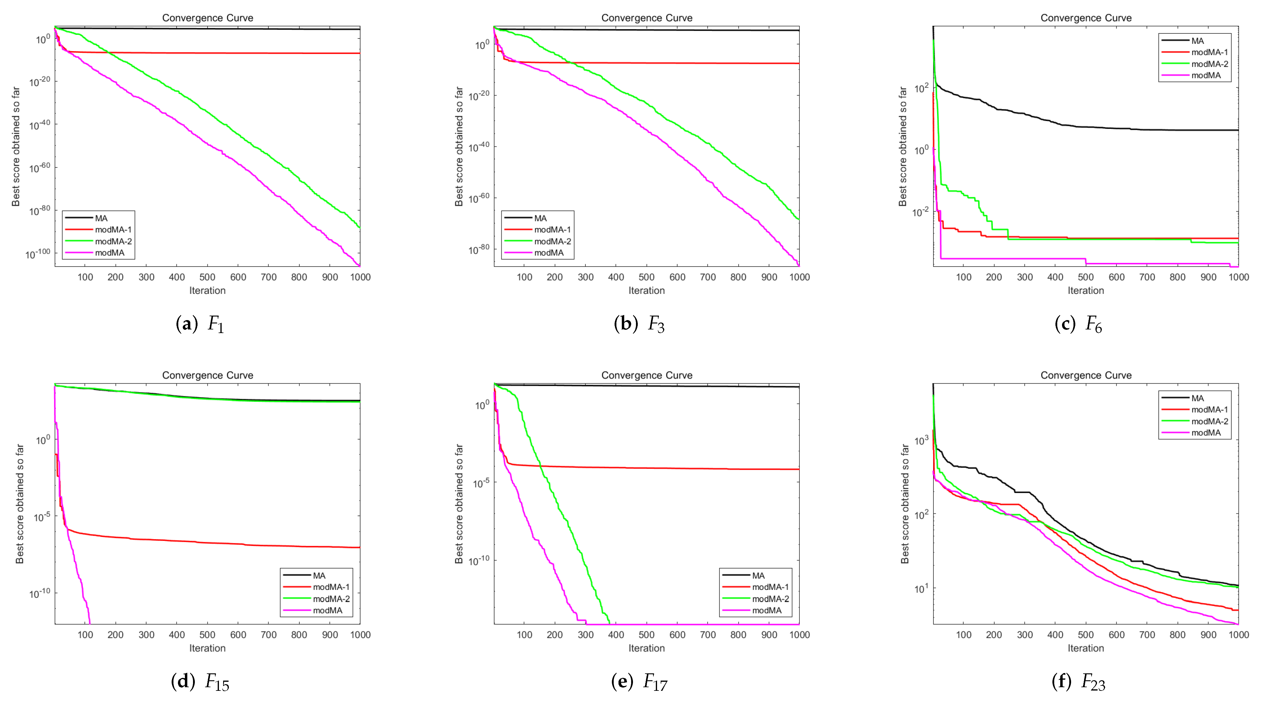
In experiment 1, we compare the performance of MA [24], modMA-1, modMA-2, and modMA on six high-dimensional functions (3 unimodal problems and 3 multimodal problems) from Table A1 and Table A2 with = 100 and = 300. It can be seen from Figure 3 and Figure 4a–f that the proposed modMA, modMA-1, modMA-2 have improved the convergence trend of the MA at high dimensions (i.e., 300 and 500), that is, modMA, modMA-1, modMA-2 can obtain better values on the benchmark functions with fewer iterations.From Figure 3c,e,f we can see that modMA has a certain level of ability in escaping from local optima values in the late iterations. From Table 2 and Table 3, the proposed modMA, modMA-1, modMA-2 can also get better results. From the and in Table 2 and Table 3, the modMA can solve the problems that MA has poor ability and instability in finding the optimal solution when solving high-dimensional complex functions.
4.3. Experiment 2: Comparison with Other Swarm Algorithms
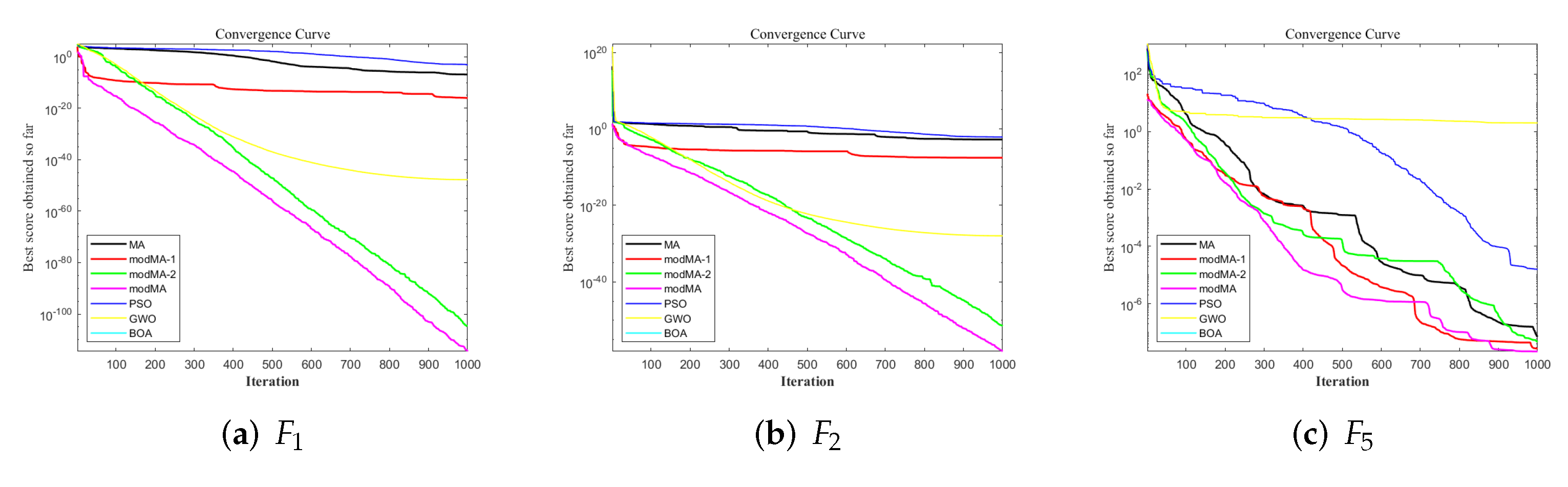
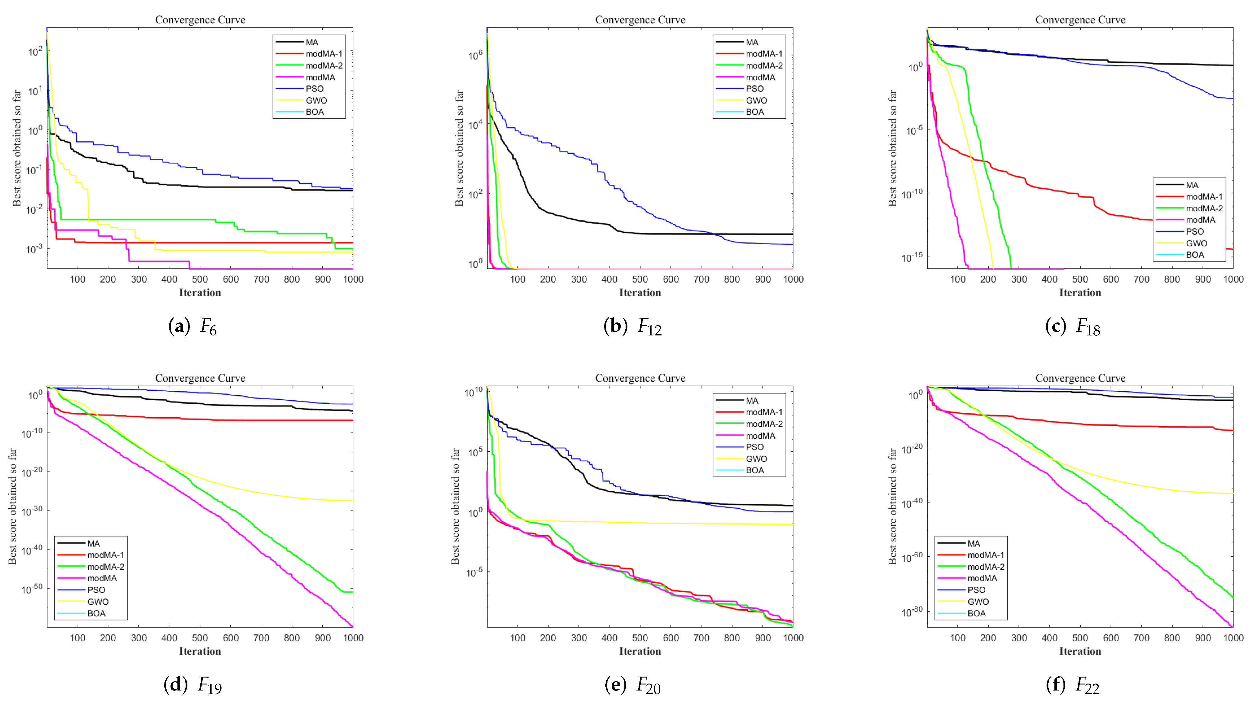
The performance of MA [24], modMA-1, modMA-2, modMA, PSO [11], GWO [20], and BOA [47] for 26 benchmark functions with = 50 is compared in this experiment. At the same time, the and the of functions are shown in Table 4.
From Table 4, the proposed modMA, modMA-1, and modMA-2 all perform well on most benchmark functions when is used as a comparison criterion.
modMA has the best performance on these 26 benchmarks functions with = 50 except , , , , and . modMA can obtain the minimum values on benchmark functions , , , , , , .
The Friedman test values and Wilcoxon sign rank test values that can reflect the difference between the proposed modMA and other algorithms (i.e., MA, modMA-1, modMA-2, PSO, GWO, and BOA) are also given in Table 5 and Table 6. Note, the significant level is set to 0.05. This signifies that the sample result is not statistically significant if the p-value is larger than 0.05.
In addition, we also select the convergence curves of various algorithms on some benchmark functions to visually show the degree of convergence of the modMA-1, modMA-2, and modMA, as shown in Figure 5 and Figure 6. Compared with MA, the convergence accuracy of the proposed modMA-1, modMA-2, and modMA is significantly improved. Compared to modMA-1 and modMA-2, modMA converges faster and finds the global optimum with fewer iterations in most functions. On the whole, modMA can effectively improve the capability of exploitation, exploration, and stability of MA. modMA also has a better convergence rate and accuracy than other algorithms.
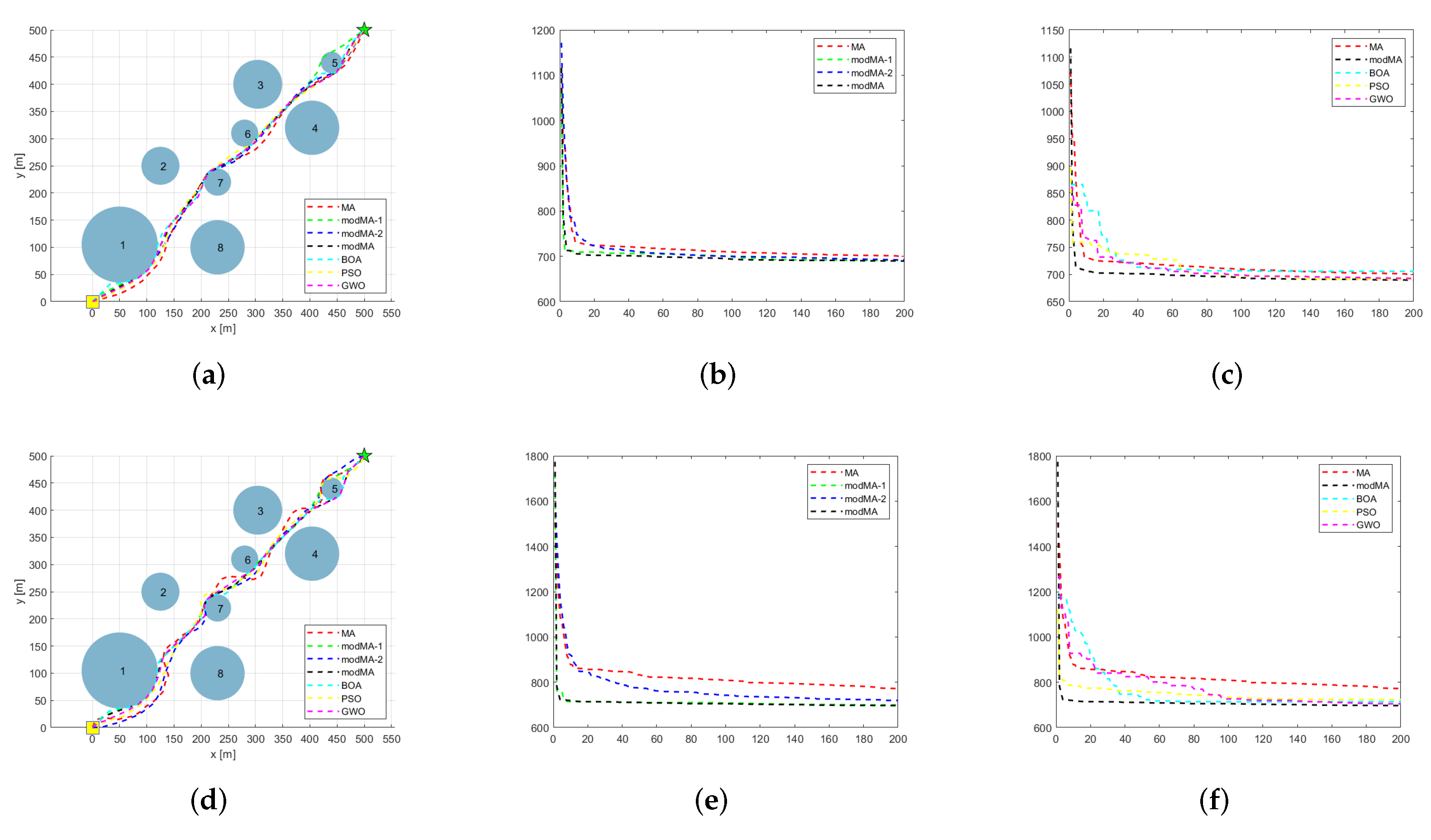
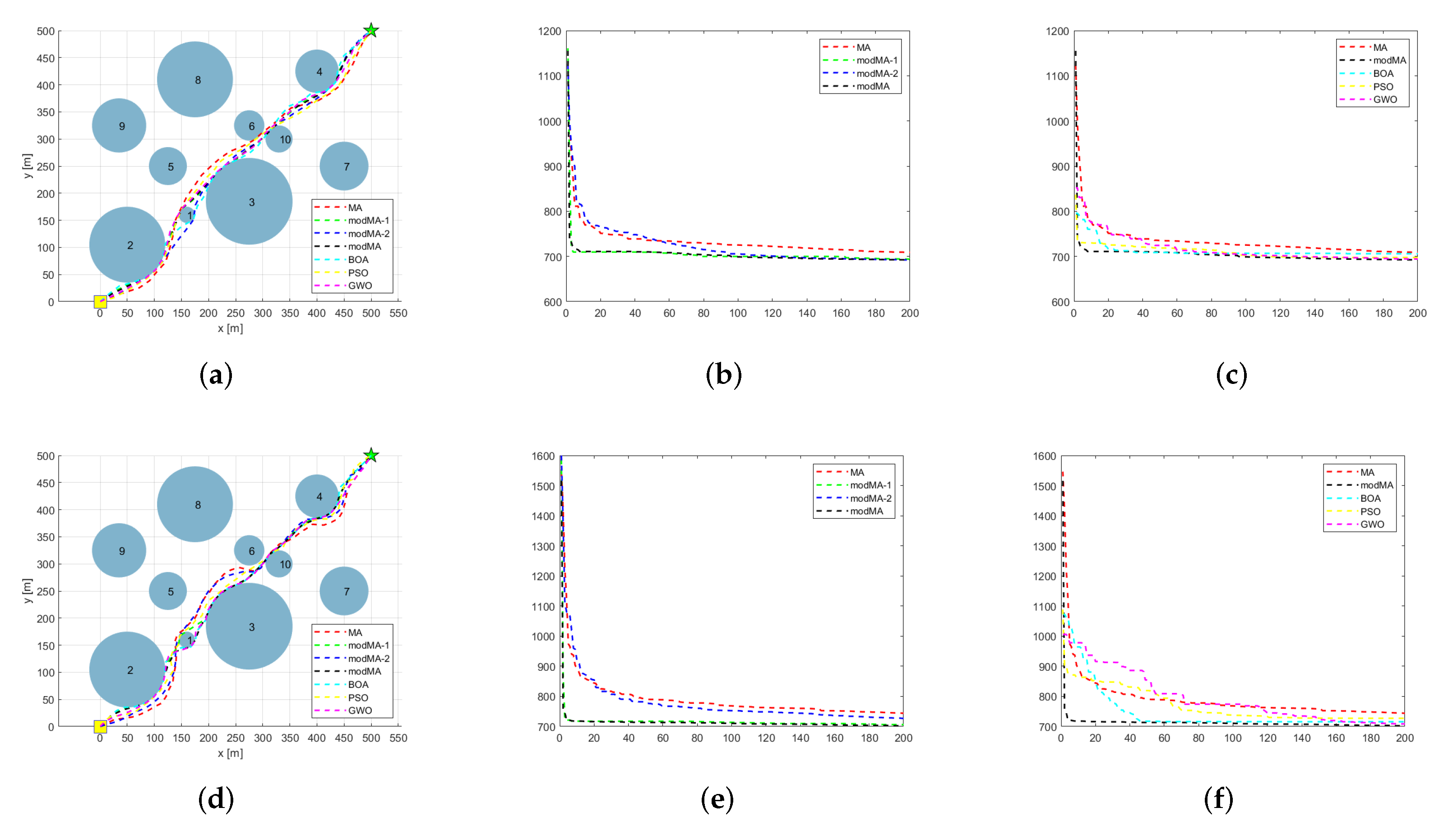
4.4. Uav Path Planning Experiment
In this section, the proposed modMA is evaluated in two separate scenarios, the threat locations for the two cases are listed in Table 7. We select PSO [11], GWO [20], BOA [47], MA [24], modMA-1, modMA-2, and modMA for experiments. The parameter settings of these algorithms are the same as in Section 4.1.
In both cases, we assume that the start point and target point of the drone are (0, 0), and (500, 500). The maximum turning angle is set to 45 degrees. The values of weight coefficients and are set to 0.95 and 0.05, respectively. This paper discusses D = 30 and D = 50 in each scenario separately. D is set to 50, that is, the distance between the start point and target point is cut into 50 segments. To guarantee equality of the comparison, the number of particles, the pre-defined maximum iteration value, and each algorithm’s number of runs are all set to 40, 200, and 30.
The experimental results are listed in Table 8. The corresponding convergence curves are shown in Figure 7a–f and Figure 8a–f. From Figure 7a–f and Figure 8a–f, all the seven algorithms can find collision-free flight paths, but they perform differently in terms of path length and smoothness. It can be seen from Table 8 that in the case of D = 30, that is, in a lower dimension, each algorithm can achieve good results, and the path length planned by modMA is shorter and the path is smoother. In the case of D = 50, that is, in a higher dimension, modMA, modMA-1, and modMA-2 greatly improve the performance of MA. modMA and modMA-1 can achieve better results in most cases, and both have good initial solutions and convergence rates, but the fluctuation of modMA is smaller than that of modMA-1. Among all the comparison algorithms, the overall cost of modMA planning is the smallest in most cases, which shows that the path planned by the modMA can reach the best when the UAV avoids collision, which proves the effectiveness of the modMA.
The path planning problem has many local solutions, this makes classical optimization techniques difficult to solve. modMA shows excellent performance on this complex problem, i.e., the quality of the solution and the stability of the solution. In addition, modMA also has good initial solution and fast convergence speed. However, the model established in this paper still has some shortcomings. After collision handling, that is, the operation of moving the waypoint to the edge of the obstacle, the planned path length may be longer than the theoretical optimum.
5. Conclusions
A new algorithm modMA which incorporates a mixed strategy consisting of three improved techniques is proposed throughout this research for solving the UAV path planning problem. By introducing the EDIW strategy to balance the particles’ processes of exploration and exploitation. By perturbing the position of each male particle with an adaptive Cauchy mutation operator, the diversity of the swarm is increased. By introducing an enhanced crossover operator, the exploration ability of the modMA is enhanced. To assess the efficacy of these three improvement techniques on MA, two experiments are designed. The suggested modMA is tested on 26 benchmark functions, and it has obvious advantages in finding both the best value and convergence speed. Finally, the proposed modMA, together with PSO, GWO, and BOA, are applied to the UAV path planning problem; simulation experiments show that the effect of modMA which is applied to the UAV path planning problem is relatively stable, and the quality of the planned path is high. The time cost of modMA in the path planning problem of UAV is higher than that of PSO, BOA and GWO, which is determined by its algorithm structure, but the the convergence speed is fast in the process of solving the problem.
Author Contributions
Conceptualization, X.W. and J.-S.P.; Formal analysis, X.W., J.-S.P., Q.Y. and S.-C.C.; Methodology, X.W., J.-S.P., L.K., V.S. and S.-C.C.; Validation, J.-S.P., Q.Y., L.K. and V.S.; Writing—original draft, X.W.; Writing—review & editing, X.W., J.-S.P., Q.Y., L.K., V.S. and S.-C.C. All authors have read and agreed to the published version of the manuscript.
Funding
This research received no external funding.
Institutional Review Board Statement
Not applicable.
Informed Consent Statement
Not applicable.
Data Availability Statement
Not applicable.
Conflicts of Interest
The authors declare no conflict of interest of this paper.
Appendix A

Table A1.
Unimodal benchmark functions.
| Name | Formula of Functions | Dim | Range | |
|---|---|---|---|---|
| Sphere | 50 | [−100, 100] | 0 | |
| Schwefel 2.22 | 50 | [−10, 10] | 0 | |
| Schwefel 1.2 | 50 | [−100, 100] | 0 | |
| Schwefel 2.21 | 50 | [−10, 10] | 0 | |
| Step | 50 | [−10, 10] | 0 | |
| Quartic | 50 | [−1.28, 1.28] | 0 | |
| Exponential | 50 | [−10, 10] | 0 | |
| Sum power | 50 | [−1, 1] | 0 | |
| Sum square | 50 | [−10, 10] | 0 | |
| Rosenbrock | 50 | [−5, 10] | 0 | |
| Zakharov | 50 | [−5, 10] | 0 | |
| Trid | 50 | [−10, 10] | 0 | |
| Elliptic | 50 | [−100, 100] | 0 | |
| Cigar | 50 | [−100, 100] | 0 |
Table A2.
Multimodal benchmark functions.
| Name | Formula of Functions | Dim | Range | |
|---|---|---|---|---|
| Rastrigin | 50 | [−5.12, 5.12] | 0 | |
| NCRastrigin | 50 | [−5.12, 5.12] | 0 | |
| Ackley | 50 | [−50, 50] | 0 | |
| Griewank | 50 | [−600, 600] | 0 | |
| Alpine | 50 | [−10, 10] | 0 | |
| Penalized 1 | 50 | [−100, 100] | 0 | |
| Penalized 2 | 50 | [−100, 100] | 0 | |
| Schwefel | 50 | [−100, 100] | 0 | |
| Levy | 50 | [−10, 10] | 0 | |
| Weierstrass | 50 | [−1, 1] | 0 | |
| Solomon | 50 | [−100, 100] | 0 | |
| Bohachevsky | 50 | [−10, 10] | 0 |
References
- Yu, X.; Zhang, Y. Sense and avoid technologies with applications to unmanned aircraft systems: Review and prospects. Prog. Aerosp. Sci. 2015, 74, 152–166. [Google Scholar] [CrossRef]
- Huo, L.; Zhu, J.; Wu, G.; Li, Z. A novel simulated annealing based strategy for balanced UAV task assignment and path planning. Sensors 2020, 20, 4769. [Google Scholar] [CrossRef] [PubMed]
- Dhulkefl, E.J.; Durdu, A. Path planning algorithms for unmanned aerial vehicles. Int. J. Trend Sci. Res. Dev. 2019, 3, 359–362. [Google Scholar] [CrossRef]
- Zhang, Z.; Wu, J.; Dai, J.; He, C. A novel real-time penetration path planning algorithm for stealth UAV in 3D complex dynamic environment. IEEE Access 2020, 8, 122757–122771. [Google Scholar] [CrossRef]
- Zhang, D.; Xu, Y.; Yao, X. An improved path planning algorithm for unmanned aerial vehicle based on rrt-connect. In Proceedings of the 2018 37th Chinese Control Conference (CCC), Wuhan, China, 25–27 July 2018; pp. 4854–4858. [Google Scholar]
- Huo, L.; Zhu, J.; Li, Z.; Ma, M. A hybrid differential symbiotic organisms search algorithm for UAV path planning. Sensors 2021, 21, 3037. [Google Scholar] [CrossRef] [PubMed]
- Zhang, D.; Duan, H. Social-class pigeon-inspired optimization and time stamp segmentation for multi-UAV cooperative path planning. Neurocomputing 2018, 313, 229–246. [Google Scholar] [CrossRef]
- Zhang, X.; Duan, H. An improved constrained differential evolution algorithm for unmanned aerial vehicle global route planning. Appl. Soft Comput. 2015, 26, 270–284. [Google Scholar] [CrossRef]
- Rajabioun, R. Cuckoo optimization algorithm. Appl. Soft Comput. 2011, 11, 5508–5518. [Google Scholar] [CrossRef]
- Song, P.C.; Pan, J.S.; Chu, S.C. A parallel compact cuckoo search algorithm for three-dimensional path planning. Appl. Soft Comput. 2020, 94, 106443. [Google Scholar] [CrossRef]
- Kennedy, J.; Eberhart, R. Particle swarm optimization. In Proceedings of the ICNN’95-International Conference on Neural Networks, Perth, WA, USA, 27 November–1 December 1995; Volume 4, pp. 1942–1948. [Google Scholar]
- Chu, S.C.; Roddick, J.F.; Pan, J.S. A parallel particle swarm optimization algorithm with communication strategies. J. Inf. Sci. Eng. 2005, 21, 809–818. [Google Scholar]
- Phung, M.D.; Ha, Q.P. Safety-enhanced UAV path planning with spherical vector-based particle swarm optimization. Appl. Soft Comput. 2021, 107, 107376. [Google Scholar] [CrossRef]
- Mirjalili, S. Genetic algorithm. In Evolutionary Algorithms and Neural Networks; Springer: Berlin/Heidelberg, Germany, 2019; pp. 43–55. [Google Scholar]
- Roberge, V.; Tarbouchi, M.; Labonté, G. Comparison of parallel genetic algorithm and particle swarm optimization for real-time UAV path planning. IEEE Trans. Ind. Info. 2012, 9, 132–141. [Google Scholar] [CrossRef]
- Basturk, B. An artificial bee colony (ABC) algorithm for numeric function optimization. In Proceedings of the IEEE Swarm Intelligence Symposium, Indianapolis, IN, USA, 12–14 May 2006. [Google Scholar]
- Lei, L.; Shiru, Q. Path planning for unmanned air vehicles using an improved artificial bee colony algorithm. In Proceedings of the 31st Chinese Control Conference, Hefei, China, 25–27 July 2012; pp. 2486–2491. [Google Scholar]
- Price, K.V. Differential evolution: A fast and simple numerical optimizer. In Proceedings of the North American Fuzzy Information Processing, Berkeley, CA, USA, 19–22 June 1996; pp. 524–527. [Google Scholar]
- Pan, J.S.; Liu, N.; Chu, S.C. A hybrid differential evolution algorithm and its application in unmanned combat aerial vehicle path planning. IEEE Access 2020, 8, 17691–17712. [Google Scholar] [CrossRef]
- Mirjalili, S.; Mirjalili, S.M.; Lewis, A. Grey wolf optimizer. Adv. Eng. Softw. 2014, 69, 46–61. [Google Scholar] [CrossRef] [Green Version]
- Lv, J.X.; Yan, L.J.; Chu, S.C.; Cai, Z.M.; Pan, J.S.; He, X.K.; Xue, J.K. A new hybrid algorithm based on golden eagle optimizer and grey wolf optimizer for 3D path planning of multiple UAVs in power inspection. Neural Comput. Appl. 2022, 193, 509–532. [Google Scholar] [CrossRef]
- Dorigo, M.; Birattari, M.; Stutzle, T. Ant colony optimization. IEEE Comput. Intell. Mag. 2006, 1, 28–39. [Google Scholar] [CrossRef]
- Konatowski, S.; Pawłowski, P. Ant colony optimization algorithm for UAV path planning. In Proceedings of the 2018 14th International Conference on Advanced Trends in Radioelecrtronics, Telecommunications and Computer Engineering (TCSET), Lviv-Slavske, Ukraine, 20–24 February 2018; pp. 177–182. [Google Scholar]
- Zervoudakis, K.; Tsafarakis, S. A mayfly optimization algorithm. Comput. Ind. Eng. 2020, 145, 106559. [Google Scholar] [CrossRef]
- Kennedy, J. Bare bones particle swarms. In Proceedings of the 2003 IEEE Swarm Intelligence Symposium, SIS’03 (Cat. No. 03EX706), Indianapolis, IN, USA, 26 April 2003; pp. 80–87. [Google Scholar]
- Juan, Z.; Zheng-Ming, G. Bare bones mayfly optimization algorithm. In Proceedings of the 2020 2nd International Conference on Machine Learning, Big Data and Business Intelligence (MLBDBI), Taiyuan, China, 23–25 October 2020; pp. 238–241. [Google Scholar]
- Shaheen, M.A.; Hasanien, H.M.; El Moursi, M.; El-Fergany, A.A. Precise modeling of PEM fuel cell using improved chaotic MayFly optimization algorithm. Int. J. Energy Res. 2021, 45, 18754–18769. [Google Scholar] [CrossRef]
- Gigras, Y.; Gupta, K.; Choudhury, K. A comparison between bat algorithm and cuckoo search for path planning. Int. J. Innov. Res. Comput. Commun. Eng. 2015, 3, 4459–4466. [Google Scholar]
- Zhang, S.; Zhou, Y.; Li, Z.; Pan, W. Grey wolf optimizer for unmanned combat aerial vehicle path planning. Adv. Eng. Softw. 2016, 99, 121–136. [Google Scholar] [CrossRef] [Green Version]
- Pan, J.S.; Liu, J.L.; Hsiung, S.C. Chaotic cuckoo search algorithm for solving unmanned combat aerial vehicle path planning problems. In Proceedings of the 2019 11th International Conference on Machine Learning and Computing, Zhuhai, China, 22–24 February 2019; pp. 224–230. [Google Scholar]
- Duan, H.; Qiao, P. Pigeon-inspired optimization: A new swarm intelligence optimizer for air robot path planning. Int. J. Intell. Comput. Cybern. 2014, 7, 24–37. [Google Scholar] [CrossRef]
- Wang, G.; Guo, L.; Duan, H.; Liu, L.; Wang, H. A modified firefly algorithm for UCAV path planning. Int. J. Hybrid Inf. Technol. 2012, 5, 123–144. [Google Scholar]
- Zhu, W.; Duan, H. Chaotic predator–prey biogeography-based optimization approach for UCAV path planning. Aerosp. Sci. Technol. 2014, 32, 153–161. [Google Scholar] [CrossRef]
- Yang, X.S. Firefly algorithm, Levy flights and global optimization. In Research and Development in Intelligent Systems XXVI; Springer: Berlin/Heideberg, Germany, 2010; pp. 209–218. [Google Scholar]
- Foo, J.L.; Knutzon, J.; Kalivarapu, V.; Oliver, J.; Winer, E. Path planning of unmanned aerial vehicles using B-splines and particle swarm optimization. J. Aerosp. Comput. Inf. Commun. 2009, 6, 271–290. [Google Scholar] [CrossRef]
- Shi, Y.; Eberhart, R. A modified particle swarm optimizer. In Proceedings of the 1998 IEEE International Conference on Evolutionary Computation Proceedings, IEEE World Congress on Computational Intelligence (Cat. No. 98TH8360), Anchorage, AK, USA, 4–9 May 1998; pp. 69–73. [Google Scholar]
- Nickabadi, A.; Ebadzadeh, M.M.; Safabakhsh, R. A novel particle swarm optimization algorithm with adaptive inertia weight. Appl. Soft Comput. 2011, 11, 3658–3670. [Google Scholar] [CrossRef]
- Gao, Y.L.; An, X.H.; Liu, J.M. A particle swarm optimization algorithm with logarithm decreasing inertia weight and chaos mutation. In Proceedings of the 2008 International Conference on Computational Intelligence and Security, Washington, DC, USA, 13–17 December 2008; Volume 1, pp. 61–65. [Google Scholar]
- Rathore, A.; Sharma, H. Review on inertia weight strategies for particle swarm optimization. In Proceedings of Sixth International Conference on Soft Computing for Problem Solving; Springer: Berlin/Heidelberg, Germany, 2017; pp. 76–86. [Google Scholar]
- Cao, Z.; Shi, Y.; Rong, X.; Liu, B.; Du, Z.; Yang, B. Random grouping brain storm optimization algorithm with a new dynamically changing step size. In Proceedings of the International Conference in Swarm Intelligence; Springer: Berlin/Heidelberg, Germany, 2015; pp. 357–364. [Google Scholar]
- Zou, Y.; Liu, P.X.; Yang, C.; Li, C.; Cheng, Q. Collision detection for virtual environment using particle swarm optimization with adaptive cauchy mutation. Clust. Comput. 2017, 20, 1765–1774. [Google Scholar] [CrossRef]
- Chakraborty, F.; Roy, P.K.; Nandi, D. Oppositional elephant herding optimization with dynamic Cauchy mutation for multilevel image thresholding. Evol. Intell. 2019, 12, 445–467. [Google Scholar] [CrossRef]
- Fogarty, T.C. Varying the Probability of Mutation in the Genetic Algorithm. In Proceedings of the 3rd International Conference on Genetic Algorithms, Fairfax, VA, USA, 4–7 June 1989; Morgan Kaufmann Publishers Inc.: San Francisco, CA, USA, 1989; pp. 104–109. [Google Scholar]
- Lin, W.Y.; Lee, W.Y.; Hong, T.P. Adapting Crossover and Mutation Rates in Genetic Algorithms. J. Inf. Sci. Eng. 2003, 19, 889–903. [Google Scholar]
- Van Laarhoven, P.J.; Aarts, E.H. Simulated annealing. In Simulated Annealing: Theory and Applications; Springer: Berlin/Heidelberg, Germany, 1987; pp. 7–15. [Google Scholar]
- Meng, A.b.; Chen, Y.c.; Yin, H.; Chen, S.Z. Crisscross optimization algorithm and its application. Knowl. Based Syst. 2014, 67, 218–229. [Google Scholar] [CrossRef]
- Arora, S.; Singh, S. Butterfly optimization algorithm: A novel approach for global optimization. Soft Comput. 2019, 23, 715–734. [Google Scholar] [CrossRef]
- Zhang, M.; Long, D.; Qin, T.; Yang, J. A chaotic hybrid butterfly optimization algorithm with particle swarm optimization for high-dimensional optimization problems. Symmetry 2020, 12, 1800. [Google Scholar] [CrossRef]
- Wang, G.G.; Gandomi, A.H.; Zhao, X.; Chu, H.C.E. Hybridizing harmony search algorithm with cuckoo search for global numerical optimization. Soft Comput. 2016, 20, 273–285. [Google Scholar] [CrossRef]
- Pan, J.S.; Zhuang, J.; Liao, L.; Chu, S.C. Advanced equilibrium optimizer for electric vehicle routing problem with time windows. J. Netw. Intell. 2021, 6, 216–237. [Google Scholar]
Figure 1.
Two-dimensional representation of planning space.

Figure 2.
The post-collision processing flow. (a) ; (b) .

Figure 3.
Comparison of convergence curve between MA, modMA-1, modMA-2, and modMA with = 100.

Figure 4.
Comparison of convergence curve between MA, modMA-1, modMA-2, and modMA with = 300.

Figure 5.
Comparison of convergence curve of MA, modMA-1, modMA-2, modMA, PSO, GWO and BOA in benchmark functions , and when = 50.
Figure 5.
Comparison of convergence curve of MA, modMA-1, modMA-2, modMA, PSO, GWO and BOA in benchmark functions , and when = 50.

Figure 6.
Comparison of convergence curve between MA, modMA-1, modMA-2, modMA, PSO, GWO and BOA with in benchmark functions , , , , and Dim = 50.
Figure 6.
Comparison of convergence curve between MA, modMA-1, modMA-2, modMA, PSO, GWO and BOA with in benchmark functions , , , , and Dim = 50.

Figure 7.
Path diagram of a single run in Case 1. (a) Comparative path planning results in Case 1, = 30; (b) Evolution curves of four algorithms in Case 1, = 30; (c) Evolution curves of different algorithms in Case 1, = 30; (d) Comparative path planning results in Case 1, = 50; (e) Evolution curves of four algorithms in Case 1, = 50; (f) Evolution curves of different algorithms in Case 1, = 50.

Figure 8.
Path diagram of a single run in Case 2. (a) Comparative path planning results in Case 2, = 30. (b) Evolution curves of four algorithms in Case 2, = 30. (c) Evolution curves of different algorithms in Case 2, = 30. (d) Comparative path planning results in Case 2, = 50. (e) Evolution curves of four algorithms in Case 2, = 50. (f) Evolution curves of different algorithms in Case 2, = 50.

Table 1.
Parameter settings for the algorithms to be compared.
| No. | Name | Parameter |
|---|---|---|
| 1 | MA | = 0.9, = 0.2, = 1, = = 1.5, d = 5, = 2, = 1 |
| 2 | modMA-1 | = 0.9, = 0.2, = 1, = = 1.5, d = 5, = 2, = 1, = 0.15 |
| 3 | modMA-2 | = 0.9, = 0.2, = 1, = = 1.5, d = 5, = 2, = 1 |
| 4 | modMA | = 0.9, = 0.2, = 1, = = 1.5, d = 5, = 2, = 1, = 0.15 |
| 5 | PSO | = 0.9, = 0.2, = = 1.5 |
| 6 | GWO | = 2, = 0 |
| 7 | BOA | = 0.8, = 0.1, = 0.01 |
Table 2.
MA, modMA-1, modMA-2, and modMA test results on the 100-dimensional functions in experiment 1.
Table 2.
MA, modMA-1, modMA-2, and modMA test results on the 100-dimensional functions in experiment 1.
| Functions | MA | modMA-1 | modMA-2 | modMA | |
|---|---|---|---|---|---|
| Best | 1.130 × | 4.798 × | 6.615 × | 1.443 × | |
| Avg | 2.586 × | 5.163 × | 2.228 × | 5.000 × | |
| Std | 1.033 × | 1.320 × | 5.748 × | 2.713 × | |
| Best | 1.049 × | 2.301 × | 3.723 × | 3.236 × | |
| Avg | 2.029 × | 1.035 × | 1.499 × | 1.783 × | |
| Std | 5.771 × | 2.889 × | 8.154 × | 9.097 × | |
| Best | 1.517 × | 1.586 × | 3.283 × | 6.919 × | |
| Avg | 92.821 × | 1.920 × | 1.120 × | 8.239 × | |
| Std | 6.322 × | 2.029 × | 5.825 × | 5.655 × | |
| Best | 4.179 × | 2.274 × | 3.084 × | 0.000 × | |
| Avg | 5.948 × | 5.983 × | 5.799 × | 0.000 × | |
| Std | 9.749 × | 1.629 × | 1.473 × | 0.000 × | |
| Best | 7.314 × | 8.795 × | 4.441 × | 4.441 × | |
| Avg | 9.007 × | 1.006 × | 5.862 × | 5.862 × | |
| Std | 9.048 × | 1.516 × | 1.770 × | 1.770 × | |
| Best | 1.762 × | 1.652 × | 1.483 × | 1.366 × | |
| Avg | 6.624 × | 4.767 × | 3.482 × | 2.002 × | |
| Std | 1.275 × | 6.518 × | 8.994 × | 3.296 × | |
Table 3.
MA, modMA-1, modMA-2, and modMA test results on the 300-dimensional functions in experiment 1.
Table 3.
MA, modMA-1, modMA-2, and modMA test results on the 300-dimensional functions in experiment 1.
| Functions | MA | modMA-1 | modMA-2 | modMA | |
|---|---|---|---|---|---|
| Best | 1.223 × | 4.977 × | 4.135 × | 1.469 × | |
| Avg | 1.607 × | 1.547 × | 9.198 × | 4.037 × | |
| Std | 1.865 × | 5.898 × | 3.814 × | 2.206 × | |
| Best | 1.405 × | 1.363 × | 9.877 × | 1.422 × | |
| Avg | 2.414 × | 1.168 × | 4.772 × | 2.737 × | |
| Std | 8.673 × | 4.095 × | 2.340 × | 1.495 × | |
| Best | 2.985 × | 1.681 × | 2.015 × | 6.201 × | |
| Avg | 3.827 × | 2.248 × | 1.273 × | 8.106 × | |
| Std | 5.001 × | 2.093 × | 6.273 × | 5.993 × | |
| Best | 1.868 × | 6.366 × | 1.249 × | 0.000 × | |
| Avg | 2.351 × | 2.824 × | 2.269 × | 0.000 × | |
| Std | 2.567 × | 1.187 × | 4.775 × | 0.000 × | |
| Best | 1.245 × | 9.821 × | 4.441 × | 4.441 × | |
| Avg | 1.337 × | 7.345 × | 6.099 × | 6.099 × | |
| Std | 4.853 × | 1.129 × | 1.741 × | 1.803 × | |
| Best | 4.761 × | 2.691 × | 3.108 × | 2.294 × | |
| Avg | 7.554 × | 4.673 × | 5.422 × | 3.979 × | |
| Std | 1.804 × | 1.061 × | 1.415 × | 8.642 × | |
Table 4.
MA, modMA-1, modMA-2, modMA, PSO, GWO, and BOA test results on the 50-dimensional functions in experiment 2.
Table 4.
MA, modMA-1, modMA-2, modMA, PSO, GWO, and BOA test results on the 50-dimensional functions in experiment 2.
| Functions | MA | modMA-1 | modMA-2 | modMA | PSO | GWO | BOA | |
|---|---|---|---|---|---|---|---|---|
| Mean | 4.778 × | 5.874 × | 2.055 × | 4.660 × | 3.555 × | 2.875 × | 1.761 × | |
| Std | 1.533 × | 1.598 × | 1.119 × | 1.82 × | 9.273 × | 2.797 × | 7.850 × | |
| Mean | 4.695 × | 7.326 × | 4.029 × | 4.294 × | 2.038 × | 1.406 × | 2.791 × | |
| Std | 7.433 × | 1.632 × | 7.881 × | 1.834 × | 3.023 × | 1.342 × | 8.588 × | |
| Mean | 1.978 × | 8.022 × | 3.506 × | 2.191 × | 2.306 × | 2.120 × | 1.773 × | |
| Std | 8.416 × | 2.235 × | 1.920 × | 1.015 × | 7.139 × | 6.684 × | 1.050 × | |
| Mean | 1.693 × | 6.127 × | 2.147 × | 3.468 × | 6.888 × | 1.802 × | 1.057 × | |
| Std | 3.424 × | 1.037 × | 9.710 × | 1.900 × | 8.100 × | 2.251 × | 4.996 × | |
| Mean | 4.184 × | 4.388 × | 4.502 × | 5.995 × | 4.134 × | 1.873 × | 1.031 × | |
| Std | 1.871 × | 2.737 × | 3.135 × | 2.724 × | 1.382 × | 5.635 × | 7.762 × | |
| Mean | 6.249 × | 1.826 × | 1.145 × | 6.490 × | 3.759 × | 1.010 × | 6.995 × | |
| Std | 1.634 × | 1.533 × | 6.072 × | 5.269 × | 1.022 × | 3.972 × | 2.370 × | |
| Mean | 2.67 × | 2.67 × | 2.67 × | 2.67 × | 0.000 × | 5.688 × | 4.816 × | |
| Std | 9.62 × | 9.62 × | 9.62 × | 9.62 × | 0.000 × | 2.500 × | 2.567 × | |
| Mean | 9.117 × | 8.800 × | 5.99 × | 1.345 × | 1.431 × | 2.35 × | 7.036 × | |
| Std | 3.569 × | 4.504 × | 0.000 × | 0.000 × | 6.681 × | 0.000 × | 8.769 × | |
| Mean | 1.857 × | 8.590 × | 9.788 × | 8.851 × | 5.935 × | 5.060 × | 1.779 × | |
| Std | 2.261 × | 2.701 × | 5.349 × | 4.84 × | 7.443 × | 9.881 × | 9.194 × | |
| Mean | 4.387 × | 4.432 × | 4.232 × | 4.214 × | 8.405 × | 4.691 × | 4.865 × | |
| Std | 4.150E × | 5.236 × | 5.382 × | 4.549 × | 5.093 × | 8.848 × | 3.134 × | |
| Mean | 1.188 × | 3.801 × | 5.403 × | 1.677 × | 3.334 × | 3.162 × | 1.781 × | |
| Std | 5.051 × | 2.081 × | 2.684 × | 6.50 × | 3.967 × | 5.144 × | 7.002 × | |
| Mean | 3.576 × | 6.667 × | 6.667 × | 6.667 × | 4.652 × | 6.667 × | 9.938 × | |
| Std | 3.066 × | 1.938 × | 1.899 × | 3.630 × | 4.149 × | 5.015 × | 2.995 × | |
| Mean | 0.000 × | 0.000 × | 0.000 × | 0.000 × | 2.10 × | 0.000 × | 8.645 × | |
| Std | 0.000 × | 0.000 × | 0.000 × | 0.000 × | 1.13 × | 0.000 × | 3.426 × | |
| Mean | 2.423 × | 0.000 × | 0.000 × | 0.000 × | 2.96 × | 0.000 × | 5.324 × | |
| Std | 1.327 × | 0.000 × | 0.000 × | 0.000 × | 1.62 × | 0.000 × | 5.818 × | |
| Mean | 2.164 × | 2.634 × | 2.189 × | 0.000 × | 9.333 × | 2.776 × | 3.790 × | |
| Std | 4.315 × | 1.725 × | 5.793 × | 0.000 × | 2.150 × | 1.073 × | 2.076 × | |
| Mean | 2.080 × | 3.878 × | 2.167 × | 0.000 × | 9.597 × | 2.067 × | 4.049 × | |
| Std | 8.058 × | 1.339 × | 7.864 × | 0.000 × | 2.736 × | 3.886 × | 1.051 × | |
| Mean | 5.000 × | 1.751 × | 6.099 × | 5.507 × | 8.183 × | 3.490 × | 1.158 × | |
| Std | 8.102 × | 8.547 × | 1.803 × | 1.656 × | 6.928 × | 7.937 × | 1.646 × | |
| Mean | 1.386 × | 1.184 × | 9.036 × | 0.000 × | 1.534 × | 0.000 × | 3.938 × | |
| Std | 2.809 × | 5.123 × | 2.856 × | 0.000 × | 2.036 × | 0.000 × | 3.047 × | |
| Mean | 2.890 × | 1.782 × | 2.272 × | 3.265 × | 5.072 × | 1.060 × | 1.652 × | |
| Std | 1.243 × | 3.270 × | 7.865 × | 1.437 × | 4.089 × | 2.878 × | 1.204 × | |
| Mean | 1.473 × | 3.536 × | 1.040 × | 5.339 × | 5.595 × | 7.583 × | 8.704 × | |
| Std | 8.628 × | 2.116 × | 3.692 × | 2.591 × | 5.458 × | 2.722 × | 1.443 × | |
| Mean | 1.095 × | 4.040 × | 1.986 × | 6.401 × | 2.134 × | 1.435 × | 4.954 × | |
| Std | 7.068 × | 3.868 × | 3.389 × | 5.245 × | 2.113 × | 3.360 × | 1.596 × | |
| Mean | 6.665 × | 2.451 × | 2.741 × | 1.077 × | 1.316 × | 1.513 × | 1.302 × | |
| Std | 2.995 × | 8.827 × | 5.282 × | 3.542 × | 1.770 × | 3.101 × | 3.949 × | |
| Mean | 1.836 × | 1.769 × | 1.900 × | 1.395 × | 8.792 × | 6.202 × | 2.488 × | |
| Std | 5.037 × | 3.862 × | 3.908 × | 1.084 × | 2.203 × | 2.122 × | 3.279 × | |
| Mean | 7.653 × | 0.000 × | 5.258 × | 0.000 × | 7.259 × | 6.534 × | 1.832 × | |
| Std | 9.000 × | 0.000 × | 8.550 × | 0.000 × | 4.673 × | 3.388 × | 2.790 × | |
| Mean | 2.261 × | 5.679 × | 3.980 × | 3.286 × | 3.177 × | 3.383 × | 7.466 × | |
| Std | 5.471 × | 4.972 × | 2.258 × | 4.553 × | 8.810 × | 1.214 × | 2.313 × | |
| Mean | 3.129 × | 4.385 × | 0.000 × | 0.000 × | 2.479 × | 0.000 × | 1.552 × | |
| Std | 1.848 × | 1.532 × | 0.000 × | 0.000 × | 4.433 × | 0.000 × | 8.417 × | |
Table 5.
Friedman test statistical results of seven algorithms.
| Function | Sum of Squares | Degree of Freedom | Mean Squares | p-Value |
|---|---|---|---|---|
| 826.667 | 6 | 137.778 | 1.372 × | |
| 770.667 | 6 | 128.444 | 4.81761 × | |
| 814.067 | 6 | 135.678 | 5.13321 × | |
| 821.333 | 6 | 136.889 | 2.39823 × | |
| 704.867 | 6 | 117.478 | 4.65662 × | |
| 591.533 | 6 | 98.5889 | 6.18862 × | |
| 690 | 6 | 115 | 3.39314 × | |
| 821.533 | 6 | 136.922 | 1.72524 × | |
| 836.267 | 6 | 139.378 | 5.01757 × | |
| 440.933 | 6 | 73.4889 | 3.53761 × | |
| 836.267 | 6 | 139.378 | 5.01757 × | |
| 730.2 | 6 | 121.7 | 3.30782 × | |
| 540 | 6 | 90 | 3.39314 × | |
| 536.233 | 6 | 89.3722 | 1.27613 × | |
| 737.65 | 6 | 122.942 | 4.72241 × | |
| 643.467 | 6 | 107.244 | 3.58476 × | |
| 742.083 | 6 | 123.681 | 4.75385 × | |
| 724.917 | 6 | 120.819 | 1.97730 × | |
| 648.467 | 6 | 108.078 | 1.66346 × | |
| 727.933 | 6 | 121.322 | 4.19129 × | |
| 683.467 | 6 | 113.911 | 4.33937 × | |
| 713.867 | 6 | 118.978 | 1.82038 × | |
| 562.667 | 6 | 93.7778 | 1.23609 × | |
| 590.25 | 6 | 98.375 | 5.55632 × | |
| 817.8 | 6 | 136.3 | 2.83026 × | |
| 719.333 | 6 | 119.889 | 8.82755 × |
Table 6.
The statistical results of the Wilcoxon rank-sum test for seven algorithms.
| Function | modMA | MA | modMA-1 | modMA-2 | PSO | GWO | BOA |
|---|---|---|---|---|---|---|---|
| 3.020 × | 3.020 × | 4.504 × | 3.020 × | 3.020 × | 3.020 × | ||
| 3.020 × | 3.020 × | 5.494 × | 3.020 × | 3.020 × | 3.020 × | ||
| 3.020 × | 3.020 × | 4.504 × | 3.020 × | 3.020 × | 3.020 × | ||
| 3.020 × | 3.020 × | 7.773 × | 3.020 × | 3.020 × | 3.020 × | ||
| 3.848 × | 2.151 × | 3.265 × | 3.020 × | 3.020 × | 3.020 × | ||
| 3.020 × | 1.518 × | 1.058 × | 3.020 × | 3.368 × | 5.369 × | ||
| 1.685 × | 1.212 × | 1.212 × | |||||
| 2.113 × | 2.113 × | 5.561 × | 2.113 × | 2.113 × | 2.113 × | ||
| 3.020 × | 3.020 × | 4.975 × | 3.020 × | 3.020 × | 3.020 × | ||
| 6.627 × | 3.020 × | 1.761 × | 1.067 × | 3.020 × | 3.020 × | ||
| 3.020 × | 3.020 × | 3.020 × | 3.020 × | 3.020 × | 3.020 × | ||
| 3.338 × | 1.273 × | 2.581 × | 3.020 × | 6.722 × | 3.020 × | ||
| 1.212 × | 1.212 × | ||||||
| 5.584 × | 1.212 × | 1.212 × | |||||
| 1.212 × | 1.836 × | 1.212 × | 1.212 × | 5.542 × | 3.337 × | ||
| 1.212 × | 1.171 × | 1.212 × | 1.212 × | 8.814 × | 2.788 × | ||
| 1.015 × | 1.015 × | 1.910 × | 1.015 × | 7.763 × | 1.014 × | ||
| 1.212 × | 1.206 × | 8.152 × | 1.212 × | 4.523 × | |||
| 3.020 × | 3.020 × | 3.690 × | 3.020 × | 3.020 × | 3.020 × | ||
| 3.020 × | 2.266 × | 5.106 × | 3.020 × | 3.020 × | 3.020 × | ||
| 3.690 × | 2.608 × | 1.529 × | 7.697 × | 5.092 × | 3.020 × | ||
| 3.020 × | 3.020 × | 4.077 × | 3.020 × | 3.020 × | 3.020 × | ||
| 1.501 × | 7.062 × | 6.627 × | 5.555 × | 3.020 × | 3.020 × | ||
| 1.212 × | 4.777 × | 1.212 × | 1.212 × | 1.455 × | |||
| 2.772 × | 9.762 × | 1.182 × | 2.930 × | 2.964 × | 2.964 × | ||
| 1.212 × | 3.428 × | 1.212 × | 1.167 × |
Table 7.
Space environment settings.
| Case Number | Serial Number | Obstacle Center | Obstacle Radius |
|---|---|---|---|
| 1 | 1 | (50, 105) | 70 |
| 2 | (125, 250) | 35 | |
| 3 | (304, 400) | 45 | |
| 4 | (404, 320) | 50 | |
| 5 | (440, 440) | 20 | |
| 6 | (280, 310) | 25 | |
| 7 | (230, 220) | 25 | |
| 8 | (230, 100) | 50 | |
| 2 | 1 | (160, 160) | 15 |
| 2 | (50, 105) | 70 | |
| 3 | (275, 185) | 80 | |
| 4 | (400, 425) | 40 | |
| 5 | (125, 250) | 35 | |
| 6 | (275, 325) | 28 | |
| 7 | (450, 250) | 45 | |
| 8 | (175, 410) | 70 | |
| 9 | (35, 325) | 50 | |
| 10 | (330, 300) | 25 |
Table 8.
The average and standard deviation values of the total cost function over thirty runs.
| Case Number | D | Results | MA | modMA-1 | modMA-2 | modMA | BOA | PSO | GWO |
|---|---|---|---|---|---|---|---|---|---|
| 1 | 30 | Avg | 705.432 | 690.146 | 692.234 | 689.532 | 711.309 | 698.138 | 693.970 |
| Std | 6.199 | 1.146 | 3.313 | 1.014 | 7.455 | 6.897 | 2.749 | ||
| 50 | Avg | 753.834 | 699.756 | 723.285 | 698.312 | 720.847 | 739.353 | 710.557 | |
| Std | 18.143 | 2.822 | 11.390 | 1.419 | 13.549 | 18.421 | 9.951 | ||
| 2 | 30 | Avg | 717.855 | 692.493 | 693.226 | 691.735 | 711.219 | 694.774 | 694.458 |
| Std | 10.718 | 1.729 | 5.087 | 1.359 | 4.180 | 3.273 | 1.675 | ||
| 50 | Avg | 781.436 | 703.315 | 747.785 | 702.119 | 721.602 | 732.321 | 710.133 | |
| Std | 28.557 | 3.123 | 23.130 | 1.978 | 6.189 | 12.167 | 7.973 |
Publisher’s Note: MDPI stays neutral with regard to jurisdictional claims in published maps and institutional affiliations. |
© 2022 by the authors. Licensee MDPI, Basel, Switzerland. This article is an open access article distributed under the terms and conditions of the Creative Commons Attribution (CC BY) license (https://creativecommons.org/licenses/by/4.0/).
Share and Cite
MDPI and ACS Style
Wang, X.; Pan, J.-S.; Yang, Q.; Kong, L.; Snášel, V.; Chu, S.-C. Modified Mayfly Algorithm for UAV Path Planning. Drones 2022, 6, 134. https://0-doi-org.brum.beds.ac.uk/10.3390/drones6050134
AMA Style
Wang X, Pan J-S, Yang Q, Kong L, Snášel V, Chu S-C. Modified Mayfly Algorithm for UAV Path Planning. Drones. 2022; 6(5):134. https://0-doi-org.brum.beds.ac.uk/10.3390/drones6050134
Chicago/Turabian StyleWang, Xing, Jeng-Shyang Pan, Qingyong Yang, Lingping Kong, Václav Snášel, and Shu-Chuan Chu. 2022. "Modified Mayfly Algorithm for UAV Path Planning" Drones 6, no. 5: 134. https://0-doi-org.brum.beds.ac.uk/10.3390/drones6050134