
UAV-Based Wetland Monitoring: Multispectral and Lidar Fusion with Random Forest Classification

Abstract
:1. Introduction
2. Materials and Methods
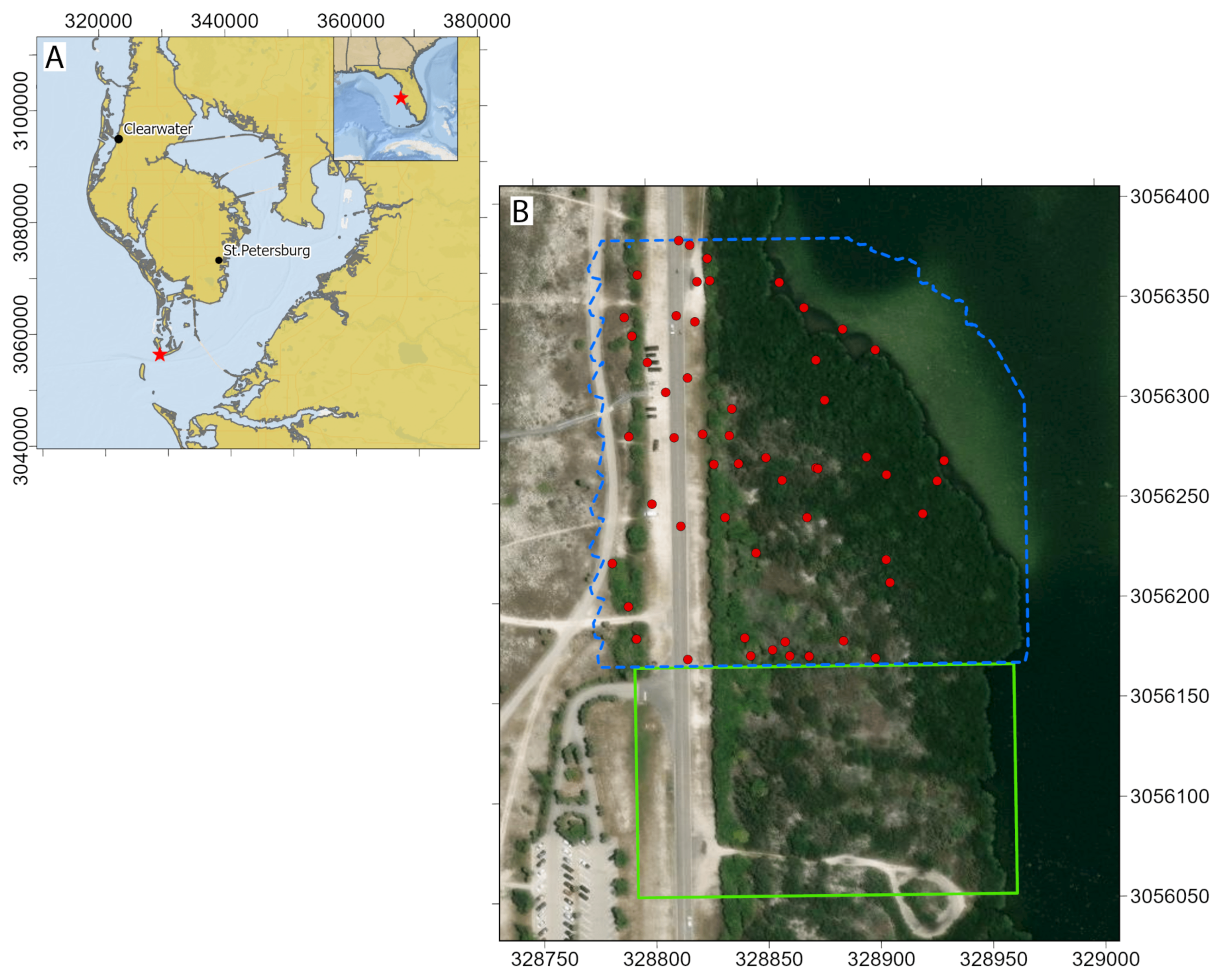
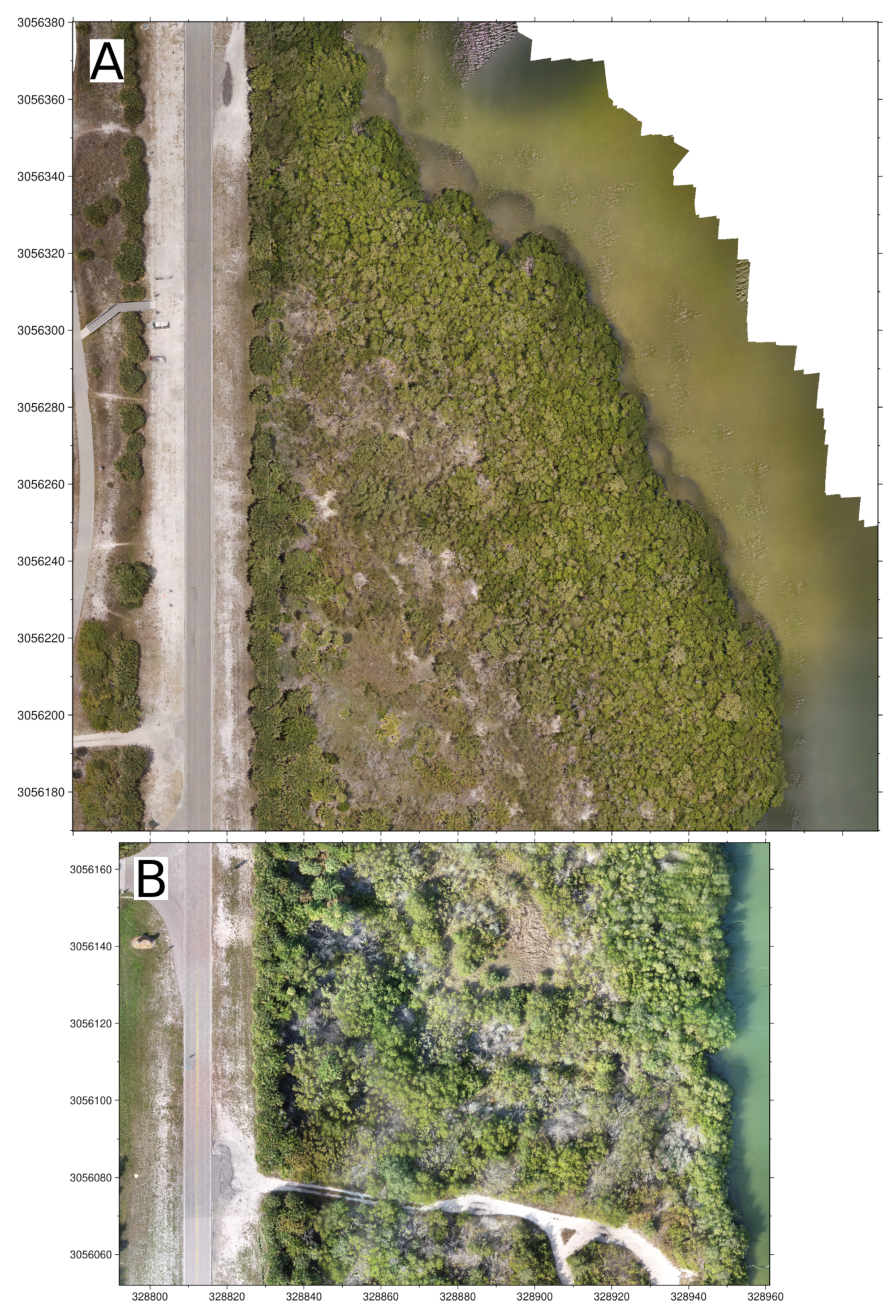
2.1. Study Area
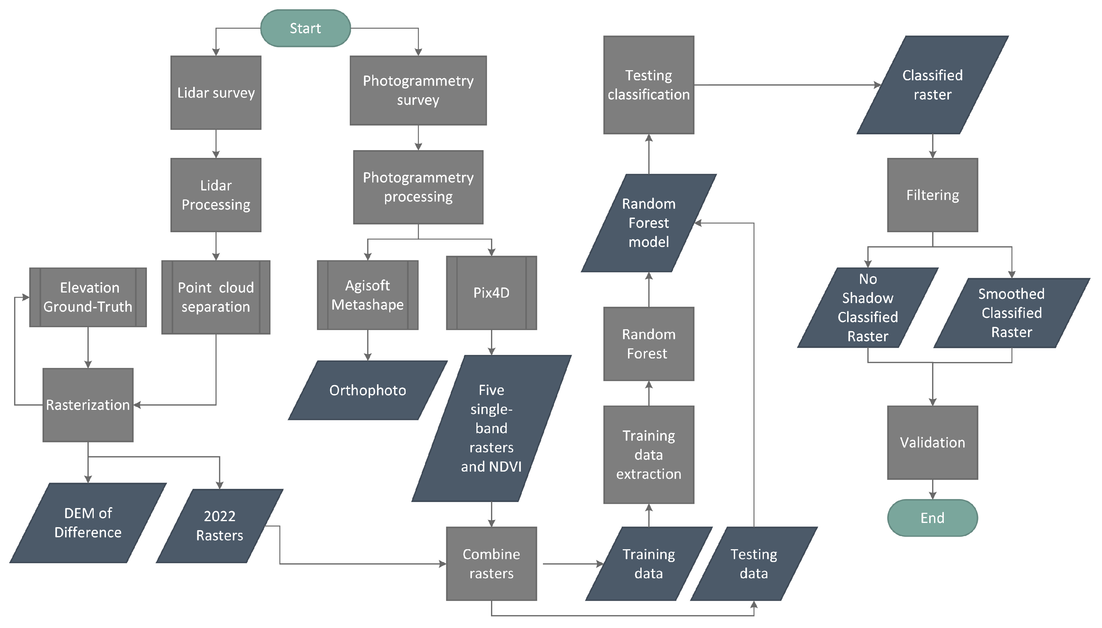
2.2. Overview
2.3. Photogrammetry and LiDAR Surveys
2.4. Photogrammetry Processing
2.5. LiDAR Processing
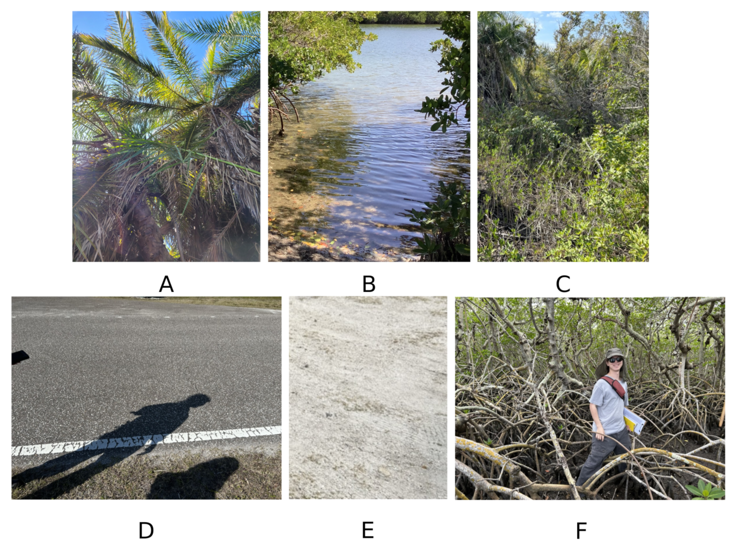
2.6. Habitat Characterization
2.7. Ground-Based Elevation Survey
2.8. Machine Learning Habitat Analysis
2.8.1. Random Forest Models
2.8.2. Training and Testing
2.8.3. Classification Map Filtering
2.8.4. Validation Habitat Characterization
2.8.5. Validation Metrics
3. Results
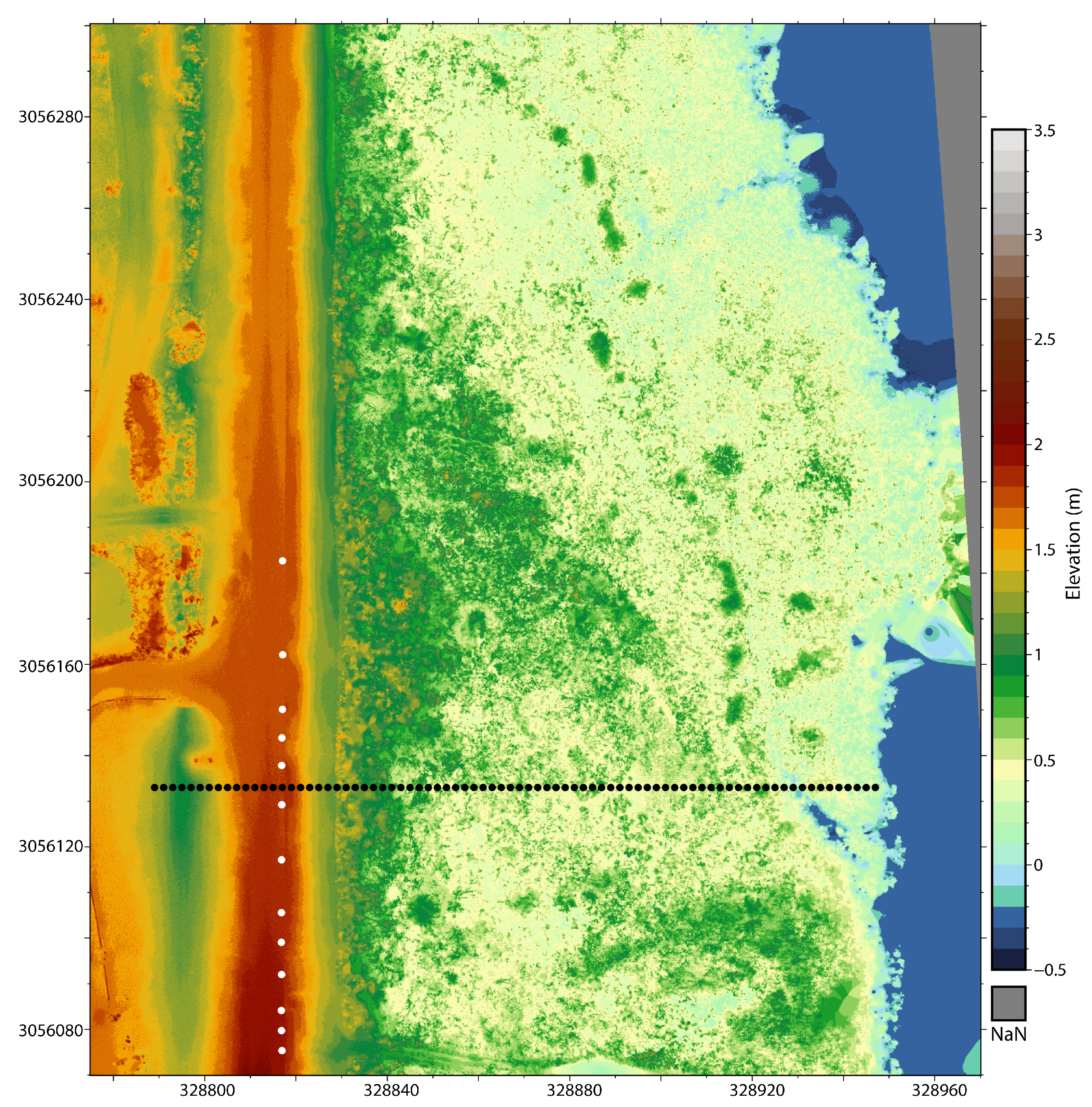
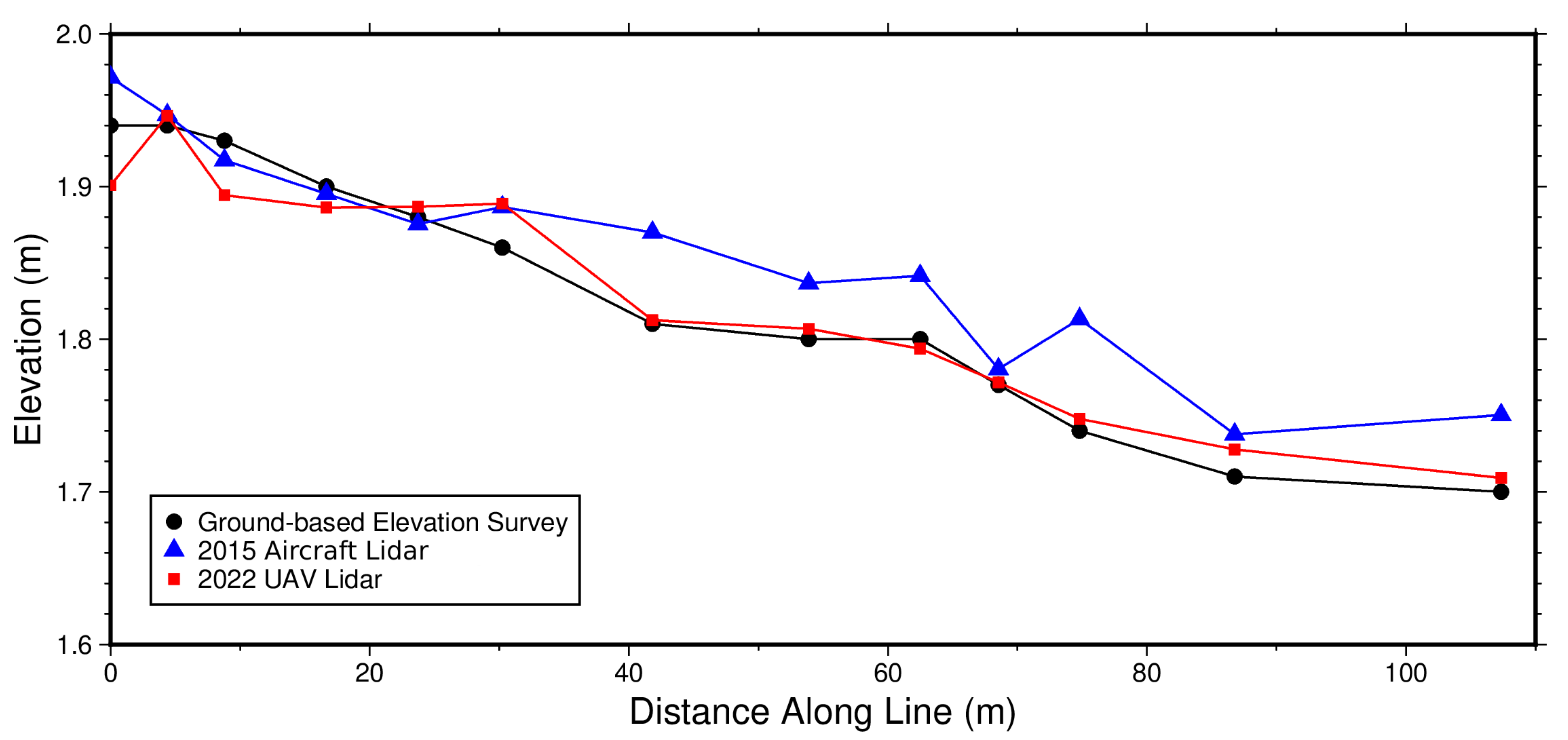
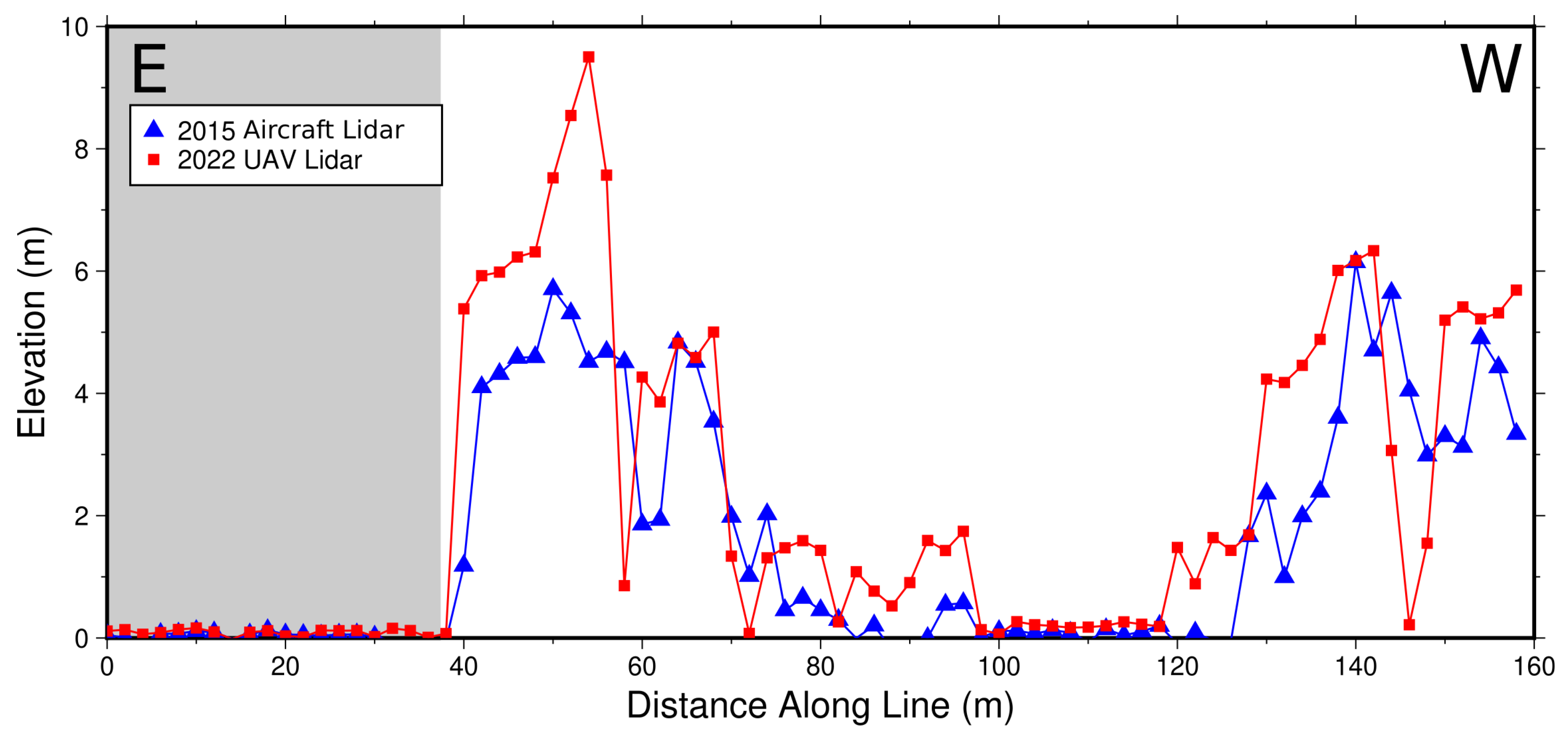
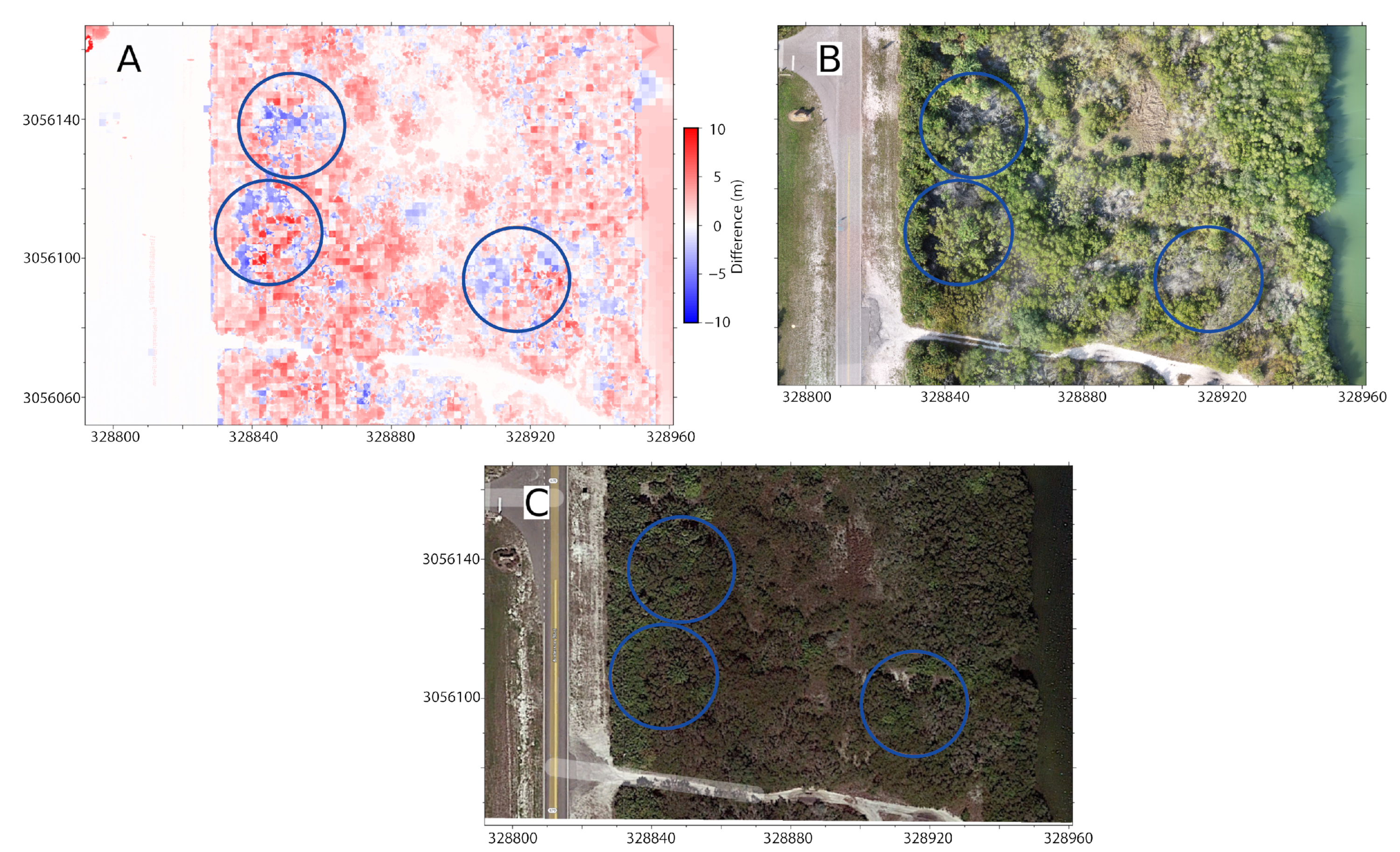
3.1. Elevation and Canopy Height Analyses
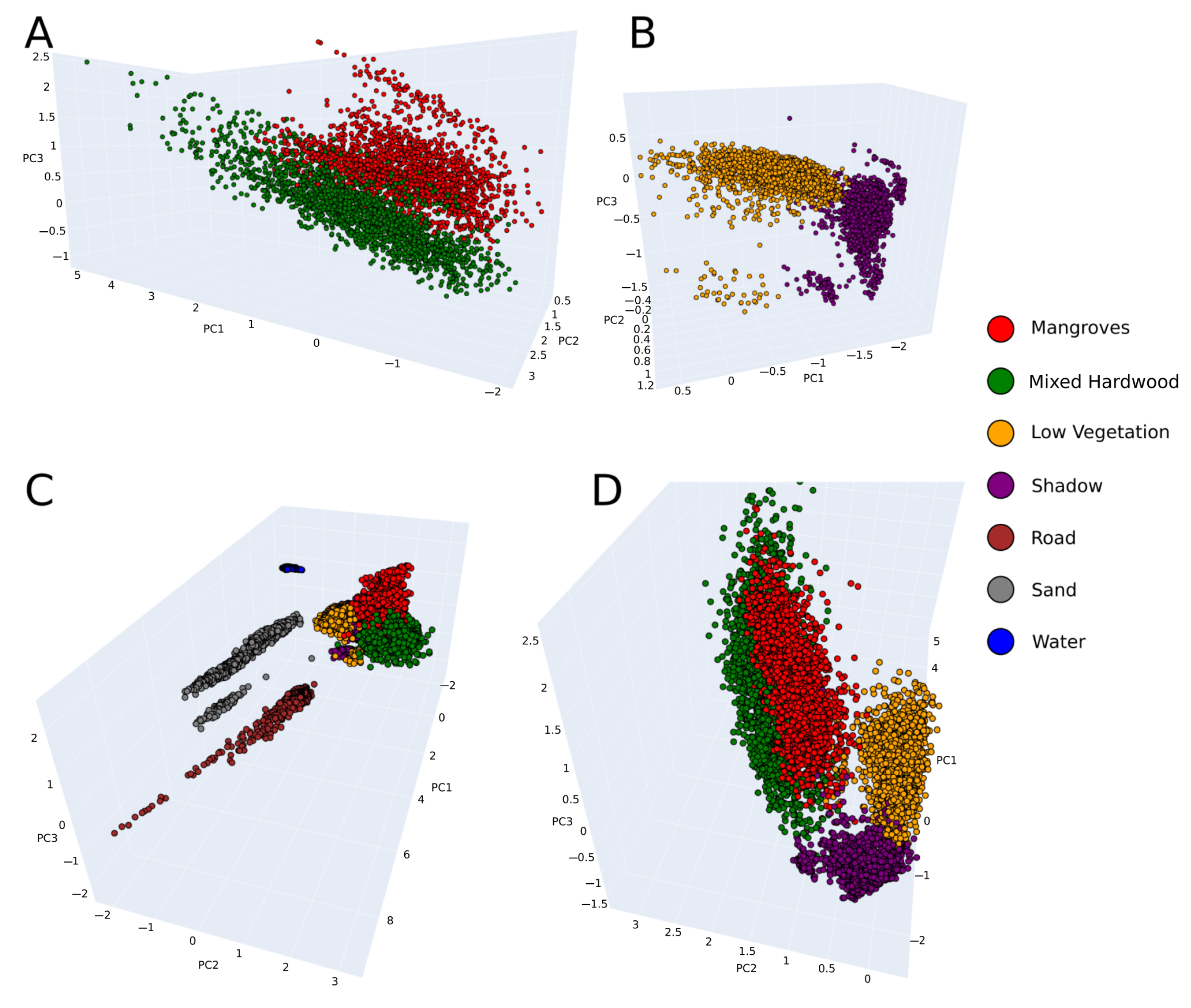
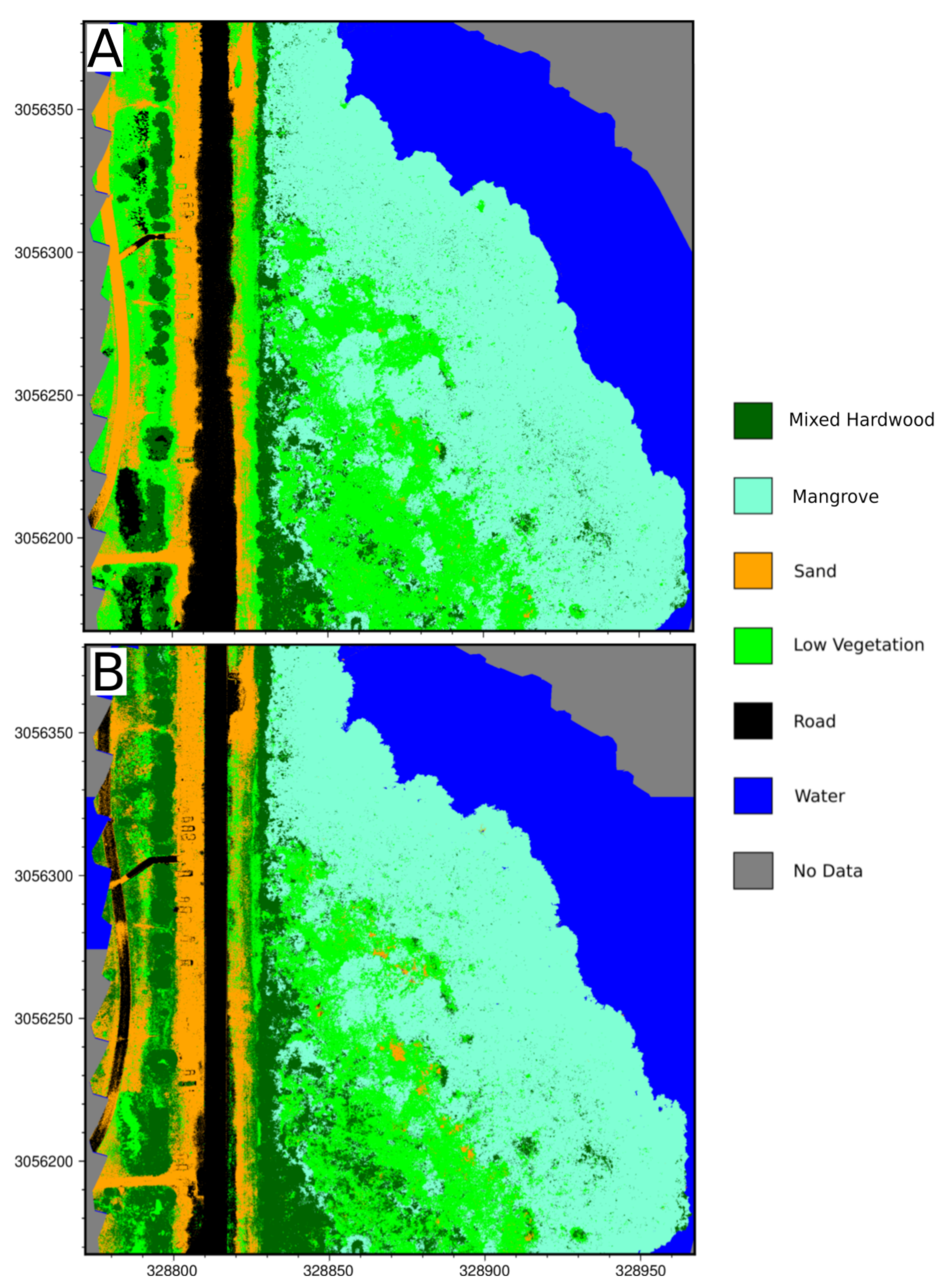
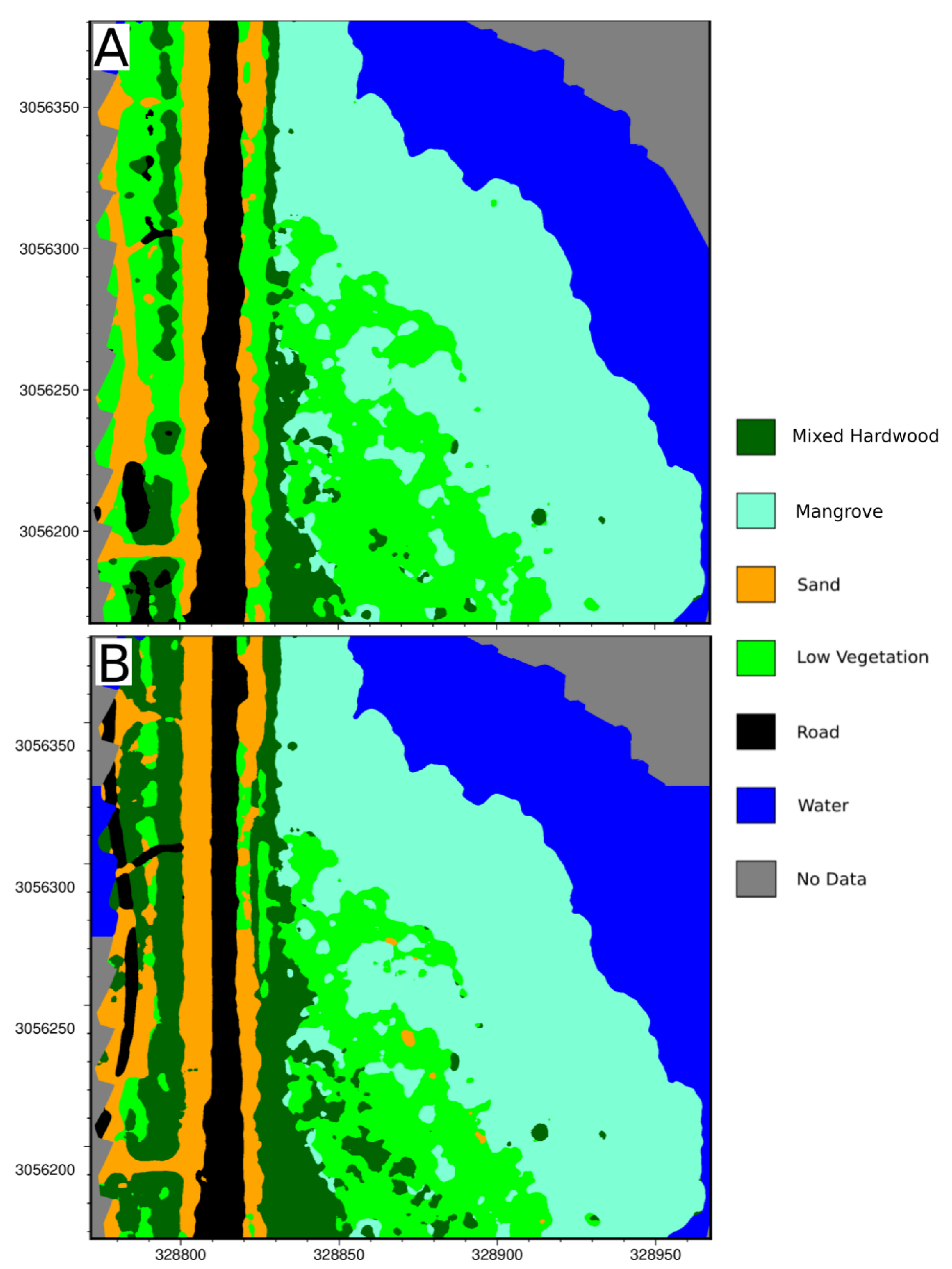
3.2. Machine Learning Habitat Classification
4. Discussion
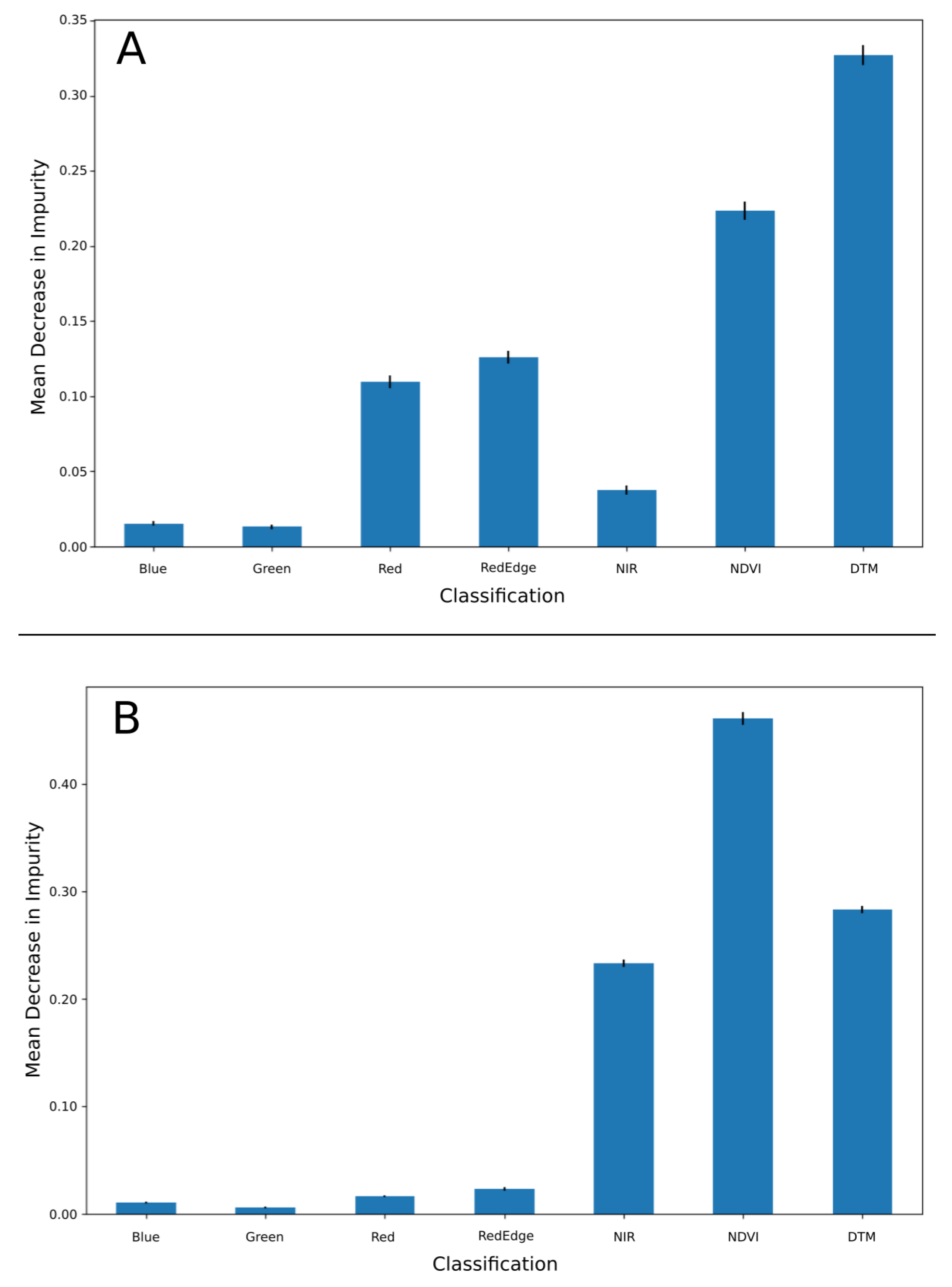
4.1. Assesment of Limiting Features and Pixel-Based Classification
4.2. Model Efficacy
4.3. Challenges and Future Work
5. Conclusions
Supplementary Materials
Author Contributions
Funding
Data Availability Statement
Acknowledgments
Conflicts of Interest
References
- Duarte, C.M.; Losada, I.J.; Hendriks, I.E.; Mazarrasa, I.; Marbà, N. The role of coastal plant communities for climate change mitigation and adaptation. Nat. Clim. Change 2013, 3, 961–968. [Google Scholar] [CrossRef]
- Fagherazzi, S.; Anisfeld, S.C.; Blum, L.K.; Long, E.V.; Feagin, R.A.; Fernandes, A.; Kearney, W.S.; Williams, K. Sea level rise and the dynamics of the marsh-upland boundary. Front. Environ. Sci. 2019, 7, 25. [Google Scholar] [CrossRef]
- Simard, M.; Fatoyinbo, L.; Smetanka, C.; Rivera-Monroy, V.H.; Castañeda-Moya, E.; Thomas, N.; Stocken, T.V.D. Mangrove canopy height globally related to precipitation, temperature and cyclone frequency. Nat. Geosci. 2019, 12, 40–45. [Google Scholar] [CrossRef]
- Feagin, R.A.; Martinez, M.L.; Mendoza-Gonzalez, G. Salt Marsh Zonal Migration and Ecosystem Service Change in Response to Global Sea Level Rise: A Case Study from an Urban Region. Ecol. Soc. 2010, 15, 4. [Google Scholar] [CrossRef]
- Rosenzweig, C.; Solecki, W.D.; Romero-Lankao, P.; Mehrotra, S.; Dhakal, S.; Ibrahim, S.A. Climate Change and Cities: Second Assessment Report of the Urban Climate Change Research Network; Cambridge University Press: Cambridge, UK, 2018. [Google Scholar]
- Fan, X.; Duan, Q.; Shen, C.; Wu, Y.; Xing, C. Global surface air temperatures in CMIP6: Historical performance and future changes. Environ. Res. Lett. 2020, 15, 104056. [Google Scholar] [CrossRef]
- Torio, D.D.; Chmura, G.L. Assessing Coastal Squeeze of Tidal Wetlands. J. Coast. Res. 2013, 29, 1049–1061. [Google Scholar] [CrossRef]
- Jafarzadeh, H.; Mahdianpari, M.; Gill, E.W.; Brisco, B.; Mohammadimanesh, F. Remote Sensing and Machine Learning Tools to Support Wetland Monitoring: A Meta-Analysis of Three Decades of Research. Remote Sens. 2022, 14, 6104. [Google Scholar] [CrossRef]
- DeLancey, E.R.; Simms, J.F.; Mahdianpari, M.; Brisco, B.; Mahoney, C.; Kariyeva, J. Comparing Deep Learning and Shallow Learning for Large-Scale Wetland Classification in Alberta, Canada. Remote Sens. 2019, 12, 2. [Google Scholar] [CrossRef]
- Sun, Z.; Jiang, W.; Ling, Z.; Zhong, S.; Zhang, Z.; Song, J.; Xiao, Z. Using Multisource High-Resolution Remote Sensing Data (2 m) with a Habitat–Tide–Semantic Segmentation Approach for Mangrove Mapping. Remote Sens. 2023, 15, 5271. [Google Scholar] [CrossRef]
- Slagter, B.; Tsendbazar, N.E.; Vollrath, A.; Reiche, J. Mapping wetland characteristics using temporally dense Sentinel-1 and Sentinel-2 data: A case study in the St. Lucia wetlands, South Africa. Int. J. Appl. Earth Obs. Geoinf. 2020, 86, 102009. [Google Scholar] [CrossRef]
- Chan-Bagot, K.; Herndon, K.E.; Nicolau, A.P.; Martín-Arias, V.; Evans, C.; Parache, H.; Mosely, K.; Narine, Z.; Zutta, B. Integrating SAR, Optical, and Machine Learning for Enhanced Coastal Mangrove Monitoring in Guyana. Remote Sens. 2024, 16, 542. [Google Scholar] [CrossRef]
- Gallant, A.L. The challenges of remote monitoring of wetlands. Remote Sens. 2015, 7, 10938–10950. [Google Scholar] [CrossRef]
- Krauss, K.W.; Mckee, K.L.; Lovelock, C.E.; Cahoon, D.R.; Saintilan, N.; Reef, R.; Chen, L. How mangrove forests adjust to rising sea level. New Phytol. 2014, 202, 19–34. [Google Scholar] [CrossRef]
- Sasmito, S.D.; Murdiyarso, D.; Friess, D.A.; Kurnianto, S. Can mangroves keep pace with contemporary sea level rise? A global data review. Wetl. Ecol. Manag. 2016, 24, 263–278. [Google Scholar] [CrossRef]
- McCarthy, M.J.; Radabaugh, K.R.; Moyer, R.P.; Muller-Karger, F.E. Enabling efficient, large-scale high-spatial resolution wetland mapping using satellites. Remote Sens. Environ. 2018, 208, 189–201. [Google Scholar] [CrossRef]
- Van Alphen, R.; Rodgers, M.; Dixon, T.H. A Technique-Based Approach to Structure-from-Motion: Applications to Human-Coastal Environments. Master’s Thesis, University of South Florida, Tampa, FL, USA, 2022. [Google Scholar]
- Rodgers, M.; Deng, F.; Dixon, T.H.; Glennie, C.L.; James, M.R.; Malservisi, R.; Van Alphen, R.; Xie, S. 2.03—Geodetic Applications to Geomorphology. In Treatise on Geomorphology; Shroder, J.F., Ed.; Academic Press: Oxford, UK, 2022; pp. 34–55. [Google Scholar] [CrossRef]
- Yang, B.; Hawthorne, T.L.; Torres, H.; Feinman, M. Using Object-Oriented Classification for Coastal Management in the East Central Coast of Florida: A Quantitative Comparison between UAV, Satellite, and Aerial Data. Drones 2019, 3, 60. [Google Scholar] [CrossRef]
- Warfield, A.D.; Leon, J.X. Estimating Mangrove Forest Volume Using Terrestrial Laser Scanning and UAV-Derived Structure-from-Motion. Drones 2019, 3, 32. [Google Scholar] [CrossRef]
- Dronova, I.; Kislik, C.; Dinh, Z.; Kelly, M. A review of unoccupied aerial vehicle use in wetland applications: Emerging opportunities in approach, technology, and data. Drones 2021, 5, 45. [Google Scholar] [CrossRef]
- Doughty, C.L.; Cavanaugh, K.C. Mapping Coastal Wetland Biomass from High Resolution Unmanned Aerial Vehicle (UAV) Imagery. Remote Sens. 2019, 11, 540. [Google Scholar] [CrossRef]
- Jeziorska, J. UAS for Wetland Mapping and Hydrological Modeling. Remote Sens. 2019, 11, 1997. [Google Scholar] [CrossRef]
- Suo, C.; McGovern, E.; Gilmer, A. Coastal Dune Vegetation Mapping Using a Multispectral Sensor Mounted on an UAS. Remote Sens. 2019, 11, 1814. [Google Scholar] [CrossRef]
- Alvarez-Vanhard, E.; Houet, T.; Mony, C.; Lecoq, L.; Corpetti, T. Can UAVs fill the gap between in situ surveys and satellites for habitat mapping? Remote Sens. Environ. 2020, 243, 111780. [Google Scholar] [CrossRef]
- Pricope, N.G.; Minei, A.; Halls, J.N.; Chen, C.; Wang, Y. UAS Hyperspatial LiDAR Data Performance in Delineation and Classification across a Gradient of Wetland Types. Drones 2022, 6, 268. [Google Scholar] [CrossRef]
- Sankey, T.; Donager, J.; McVay, J.; Sankey, J.B. UAV lidar and hyperspectral fusion for forest monitoring in the southwestern USA. Remote Sens. Environ. 2017, 195, 30–43. [Google Scholar] [CrossRef]
- Ishida, T.; Kurihara, J.; Viray, F.A.; Namuco, S.B.; Paringit, E.C.; Perez, G.J.; Takahashi, Y.; Marciano, J.J. A novel approach for vegetation classification using UAV-based hyperspectral imaging. Comput. Electron. Agric. 2018, 144, 80–85. [Google Scholar] [CrossRef]
- Cao, J.; Liu, K.; Zhuo, L.; Liu, L.; Zhu, Y.; Peng, L. Combining UAV-based hyperspectral and LiDAR data for mangrove species classification using the rotation forest algorithm. Int. J. Appl. Earth Obs. Geoinf. 2021, 102, 102414. [Google Scholar] [CrossRef]
- Quan, Y.; Li, M.; Hao, Y.; Liu, J.; Wang, B. Tree species classification in a typical natural secondary forest using UAV-borne LiDAR and hyperspectral data. GISci. Remote Sens. 2023, 60, 2171706. [Google Scholar] [CrossRef]
- Wang, D.; Wan, B.; Qiu, P.; Tan, X.; Zhang, Q. Mapping mangrove species using combined UAV-LiDAR and Sentinel-2 data: Feature selection and point density effects. Adv. Space Res. 2022, 69, 1494–1512. [Google Scholar] [CrossRef]
- Agisoft LLC. Agisoft Metashape Pro, Version 1.8.2; Agisoft LLC: St. Petersburg, Russia, 2022. [Google Scholar]
- Pix4D S.A. Pix4DMapper; Pix4D S.A.: Prilly, Switzerland, 2022. [Google Scholar]
- Kriegler, F.J. Preprocessing transformations and their effects on multspectral recognition. In Proceedings of the Sixth International Symposium on Remote Sesning of Environment, Ann Arbor, MI, USA, 13–16 October 1969; pp. 97–131. [Google Scholar]
- James, M.R.; Robson, S. Straightforward reconstruction of 3D surfaces and topography with a camera: Accuracy and geoscience application. J. Geophys. Res. Earth Surf. 2012, 117, F03017. [Google Scholar] [CrossRef]
- Cloud Compare, Version 2.11.1 GPL Software; 2022. Available online: http://www.cloudcompare.org/ (accessed on 1 February 2024).
- Zhang, W.; Qi, J.; Wan, P.; Wang, H.; Xie, D.; Wang, X.; Yan, G. An Easy-to-Use Airborne LiDAR Data Filtering Method Based on Cloth Simulation. Remote Sens. 2016, 8, 501. [Google Scholar] [CrossRef]
- OCM Partners. 2002 Florida USGS/NASA Airborne Lidar Assessment of Coastal Erosion (ALACE) Project for the US Coastline. 2002. Available online: https://www.fisheries.noaa.gov/inport/item/49631 (accessed on 11 February 2024).
- OCM Partners. 2007 Florida Division of Emergency Management (FDEM) Lidar Project: Southwest Florida. 2007. Available online: https://www.fisheries.noaa.gov/inport/item/49677 (accessed on 11 February 2024).
- OCM Partners. 2006 United States Army Corps of Engineers (USACE) Post Hurricane Wilma Lidar: Hurricane Pass to Big Hickory Pass, FL. 2006. Available online: https://www.fisheries.noaa.gov/inport/item/50059 (accessed on 11 February 2024).
- OCM Partners. 2015 USACE NCMP Topobathy Lidar: Florida Gulf Coast. 2015. Available online: https://www.fisheries.noaa.gov/inport/item/49720 (accessed on 11 February 2024).
- OCM Partners. 2015 USACE NCMP Topobathy Lidar: Egmont Key (FL). 2015. Available online: https://www.fisheries.noaa.gov/inport/item/49719 (accessed on 11 February 2024).
- Dietterich, T.G. An experimental comparison of three methods for constructing ensembles of decision trees: Bagging, boosting, and randomization. Mach. Learn. 2000, 40, 139–157. [Google Scholar] [CrossRef]
- Breiman, L. Random forests. Mach. Learn. 2001, 45, 5–32. [Google Scholar] [CrossRef]
- Caruana, R.; Niculescu-Mizil, A. An empirical comparison of supervised learning algorithms. In Proceedings of the 23rd International Conference on Machine Learning, Pittsburgh, PA, USA, 25–29 June 2006; pp. 161–168. [Google Scholar]
- Thanh Noi, P.; Kappas, M. Comparison of random forest, k-nearest neighbor, and support vector machine classifiers for land cover classification using Sentinel-2 imagery. Sensors 2017, 18, 18. [Google Scholar] [CrossRef]
- Burnett, M.; Mccauley, D.; Leo, G.A.D.; Micheli, F. Quantifying coconut palm extent on Pacific islands using spectral and textural analysis of very high resolution imagery Biogenic carbonates on sea and land View project Public Health and decision making View project. Int. J. Remote Sens. 2019, 40, 7329–7355. [Google Scholar] [CrossRef]
- Wu, N.; Shi, R.; Zhuo, W.; Zhang, C.; Tao, Z. Identification of native and invasive vegetation communities in a tidal flat wetland using gaofen-1 imagery. Wetlands 2021, 41, 46. [Google Scholar] [CrossRef]
- Pal, M. Random forest classifier for remote sensing classification. Int. J. Remote Sens. 2005, 26, 217–222. [Google Scholar] [CrossRef]
- Rodriguez-Galiano, V.F.; Ghimire, B.; Rogan, J.; Chica-Olmo, M.; Rigol-Sanchez, J.P. An assessment of the effectiveness of a random forest classifier for land-cover classification. ISPRS J. Photogramm. Remote Sens. 2012, 67, 93–104. [Google Scholar] [CrossRef]
- Pedregosa, F.; Varoquaux, G.; Gramfort, A.; Michel, V.; Thirion, B.; Grisel, O.; Blondel, M.; Prettenhofer, P.; Weiss, R.; Dubourg, V.; et al. Scikit-learn: Machine learning in Python. J. Mach. Learn. Res. 2011, 12, 2825–2830. [Google Scholar]
- Story, M.; Congalton, R.G. Accuracy assessment: A user’s perspective. Photogramm. Eng. Remote Sens. 1986, 52, 397–399. [Google Scholar]
- Congalton, R.G. Remote sensing and geographic information system data integration: Error sources and. Photogramm. Eng. Remote Sens. 1991, 57, 677–687. [Google Scholar]
- Guyon, I.; Bennett, K.; Cawley, G.; Escalante, H.J.; Escalera, S.; Ho, T.K.; Macià, N.; Ray, B.; Saeed, M.; Statnikov, A.; et al. Design of the 2015 chalearn automl challenge. In Proceedings of the 2015 International Joint Conference on Neural Networks (IJCNN), Killarney, Ireland, 12–17 July 2015; pp. 1–8. [Google Scholar]
- Cohen, A.; Sattler, T.; Pollefeys, M. Merging the Unmatchable: Stitching Visually Disconnected SfM Models. In Proceedings of the 2015 IEEE International Conference on Computer Vision (ICCV), Killarney, Ireland, 12–17 July 2015; pp. 2129–2137. [Google Scholar] [CrossRef]
- Stone, W. 2022 Is Coming—Will You Be Ready? (Or NAD83 and NAVD88 Are Going Away). 2015. Available online: https://www.ngs.noaa.gov/web/science_edu/presentations_library/files/stone_gecowest_2015_for_upload.pdf (accessed on 4 April 2023).
- Lovell, J.L.; Jupp, D.L.; Culvenor, D.S.; Coops, N.C. Using airborne and ground-based ranging lidar to measure canopy structure in Australian forests. Can. J. Remote Sens. 2003, 29, 607–622. [Google Scholar] [CrossRef]
- Heiskanen, J.; Korhonen, L.; Hietanen, J.; Heikinheimo, V.; Schäfer, E.; Pellikka, P.K.E. Comparison of field and airborne laser scanning based crown cover estimates across land cover types in Kenya. Int. Arch. Photogramm. Remote Sens. Spat. Inf. Sci. 2015, XL-7/W3, 409–415. [Google Scholar] [CrossRef]
- Wallace, L.; Lucieer, A.; Malenovský, Z.; Turner, D.; Vopěnka, P. Assessment of forest structure using two UAV techniques: A comparison of airborne laser scanning and structure from motion (SfM) point clouds. Forests 2016, 7, 62. [Google Scholar] [CrossRef]
- Fu, B.; Wang, Y.; Campbell, A.; Li, Y.; Zhang, B.; Yin, S.; Xing, Z.; Jin, X. Comparison of object-based and pixel-based Random Forest algorithm for wetland vegetation mapping using high spatial resolution GF-1 and SAR data. Ecol. Indic. 2017, 73, 105–117. [Google Scholar] [CrossRef]
- Chen, J.; Chen, Z.; Huang, R.; You, H.; Han, X.; Yue, T.; Zhou, G. The Effects of Spatial Resolution and Resampling on the Classification Accuracy of Wetland Vegetation Species and Ground Objects: A Study Based on High Spatial Resolution UAV Images. Drones 2023, 7, 61. [Google Scholar] [CrossRef]
- Musungu, K.; Dube, T.; Smit, J.; Shoko, M. Using UAV multispectral photography to discriminate plant species in a seep wetland of the Fynbos Biome. Wetl. Ecol. Manag. 2024. [Google Scholar] [CrossRef]
- Duro, D.C.; Franklin, S.E.; Dubé, M.G. A comparison of pixel-based and object-based image analysis with selected machine learning algorithms for the classification of agricultural landscapes using SPOT-5 HRG imagery. Remote Sens. Environ. 2012, 118, 259–272. [Google Scholar] [CrossRef]
- Boon, M.A.; Drijfhout, A.P.; Tesfamichael, S. Comparison of a Fixed-wing and Multi-rotor Uav for Environmental Mapping Applications: A Case Study. Int. Arch. Photogramm. Remote Sens. Spat. Inf. Sci. 2017, XLII-2/W6, 47–54. [Google Scholar] [CrossRef]
- RTKLIB: An Open Source Program Package for RTK-GPS RTKLIB software, BSD 2-Clause License. Available online: https://gpspp.sakura.ne.jp/rtklib/rtklib.htm (accessed on 1 February 2024).
- Dach, R.; Selmke, I.; Villiger, A.; Arnold, D.; Prange, L.; Schaer, S.; Sidorov, D.; Stebler, P.; Jäggi, A.; Hugentobler, U. Review of recent GNSS modelling improvements based on CODEs Repro3 contribution. Adv. Space Res. 2021, 68, 1263–1280. [Google Scholar] [CrossRef]
- Lou, Y.; Dai, X.; Gong, X.; Li, C.; Qing, Y.; Liu, Y.; Peng, Y.; Gu, S. A review of real-time multi-GNSS precise orbit determination based on the filter method. Satell. Navig. 2022, 3, 15. [Google Scholar] [CrossRef]
- Boehm, J.; Werl, B.; Schuh, H. Troposphere mapping functions for GPS and very long baseline interferometry from European Centre for Medium-Range Weather Forecasts operational analysis data. J. Geophys. Res. 2006, 111, B02406. [Google Scholar] [CrossRef]


| Channel | Center Wavelength and Bandwidth (nm) |
|---|---|
| Blue | 450 ± 16 |
| Green | 560 ± 16 |
| Red | 650 ± 16 |
| RedEdge | 730 ± 16 |
| Near-Infrared (NIR) | 840 ± 26 |
| Acquisition Dates | Horizontal Accuracy | Vertical Accuracy | Scanner | Scanner Wavelength | Scan Angle | Pulse Rate | Points per m |
|---|---|---|---|---|---|---|---|
| October 2002 | ±0.8 m | ±15 cm | ATM II | Blue-Green (523 nm) | 0° | 2–10 kHz | 0.1–0.2 |
| May–June 2006 | 80 cm at 2 sigma | 30 cm at 2 sigma | CHARTS system (SHOALS-3000 LiDAR ) | NIR (1064 nm) | 0° | n/a | 0.27 |
| June–August 2007 | ±116 cm | 9 cm RMSE | Leica ALS50 | NIR (1064 nm) | 29° | 75 kHz; 84.4 kHz | 1.8 |
| May 2015 | 1 m | 19.6 cm | CZMIL | NIR (1064 nm) | −21–22° | 10 khz | 1–14 |
| June 2015 | 1 m RMSE | 9.5 cm RMSE (topographic data only) | Leica HawkEye III | Infrared | 13–22° | 300 kHz | 0.1–0.2 |
| UAV-LiDAR, December 2022 | ±2 cm | 2 cm RMSE | Hesai Pandar XT32 | Mid-IR (905 nm) | ±30° | 3.5 MHz | 459 |
| Habitat | Number of Polygons | % of Training Area |
|---|---|---|
| Mixed Hardwood | 9 | 6.6 |
| Water | 1 | 2.4 |
| Low Vegetation | 9 | 1.6 |
| Road | 3 | 4.6 |
| Sand | 8 | 1.1 |
| Mangrove | 7 | 7 |
| Shadow | 22 | 0.5 |
| Total | 59 | 23.8 |
| Model | Number of Estimators | Max Features | Out-of-Bag Error | Tuned Model Accuracy (%) |
|---|---|---|---|---|
| 2000-point | 100 | 5 | 0.27 | 98 |
| 5000-point | 300 | 4 | 0.2 | 97 |
| Model | Balanced Average (%) | User’s Accuracy Average (%) | Producer’s Accuracy Average (%) | Kappa |
|---|---|---|---|---|
| 2000-point, no shadows | 75 | 79.3 | 76.2 | 0.70 |
| 2000-point, filtered | 78 | 80.8 | 79.2 | 0.70 |
| 5000-point, no shadows | 77 | 80.2 | 79.1 | 0.68 |
| 5000-point, filtered | 78 | 77.3 | 76.5 | 0.68 |
| Habitat | User’s Accuracy (%) | Producer’s Accuracy (%) |
|---|---|---|
| Mixed Hardwood | 100 | 54.6 |
| Water | 100 | 100 |
| Low Vegetation | 71.4 | 83.3 |
| Road | 50 | 80 |
| Sand | 83.3 | 71.4 |
| Mangrove | 80 | 85.7 |
| Habitat | 2000-Point (%) | 5000-Point (%) | 2000-Point, Filtered (%) | 5000-Point, Filtered (%) |
|---|---|---|---|---|
| Mixed Hardwood | 8.09 | 14.8 | 7.1 | 14.8 |
| Water | 19.4 | 20.6 | 19.4 | 20.6 |
| Low Vegetation | 21.8 | 14.9 | 22.5 | 14.2 |
| Road | 7.6 | 6.3 | 7.6 | 6.5 |
| Sand | 8.7 | 10 | 8.4 | 10.1 |
| Mangrove | 34.2 | 33.3 | 34.8 | 33.6 |
Disclaimer/Publisher’s Note: The statements, opinions and data contained in all publications are solely those of the individual author(s) and contributor(s) and not of MDPI and/or the editor(s). MDPI and/or the editor(s) disclaim responsibility for any injury to people or property resulting from any ideas, methods, instructions or products referred to in the content. |
© 2024 by the authors. Licensee MDPI, Basel, Switzerland. This article is an open access article distributed under the terms and conditions of the Creative Commons Attribution (CC BY) license (https://creativecommons.org/licenses/by/4.0/).
Share and Cite
Van Alphen, R.; Rains, K.C.; Rodgers, M.; Malservisi, R.; Dixon, T.H. UAV-Based Wetland Monitoring: Multispectral and Lidar Fusion with Random Forest Classification. Drones 2024, 8, 113. https://0-doi-org.brum.beds.ac.uk/10.3390/drones8030113
Van Alphen R, Rains KC, Rodgers M, Malservisi R, Dixon TH. UAV-Based Wetland Monitoring: Multispectral and Lidar Fusion with Random Forest Classification. Drones. 2024; 8(3):113. https://0-doi-org.brum.beds.ac.uk/10.3390/drones8030113
Chicago/Turabian StyleVan Alphen, Robert, Kai C. Rains, Mel Rodgers, Rocco Malservisi, and Timothy H. Dixon. 2024. "UAV-Based Wetland Monitoring: Multispectral and Lidar Fusion with Random Forest Classification" Drones 8, no. 3: 113. https://0-doi-org.brum.beds.ac.uk/10.3390/drones8030113