


Modeling of the Flight Performance of a Plasma-Propelled Drone: Limitations and Prospects

1
Institut PPRIME, Université de Poitiers, 11 Boulevard Marie et Pierre Curie, 86073 Poitiers, CEDEX 9, France
2
ISAE-SUPAERO, Université de Toulouse, 10 Avenue Edouard Belin BP 54032, 31055 Toulouse, CEDEX 4, France
*
Authors to whom correspondence should be addressed.
Drones 2024, 8(3), 114; https://0-doi-org.brum.beds.ac.uk/10.3390/drones8030114
Submission received: 5 February 2024
/
Revised: 15 March 2024
/
Accepted: 18 March 2024
/
Published: 21 March 2024
(This article belongs to the Topic Innovation and Inventions in Aerospace and UAV Applications)
Abstract
:The resurgence in interest in aircraft electro-aerodynamic (EAD) propulsion has been sparked due to recent advancements in EAD thrusters, which generate thrust by employing a plasma generated through electrical discharge. With potentially quieter propulsion that could contribute to the generation of lift or the control of attitude, it is important to determine the feasibility of an EAD-propelled airplane. First, the main propulsive characteristics (thrust generation and power consumption) of EAD thrusters were drawn from the literature and compared with existing technologies. Second, an algorithm was developed to couple standard equations of flight with EAD propulsion performance and treat the first-order interactions. It fairly replicated the performance of the only available autonomous EAD-propelled drone. A test case based on an existing commercial UAV of 10 kg equipped with current-generation EAD thrusters anticipated a flight of less than 10 min, lower than 30 m in height, and below 8 m · s −1 in velocity. Achieving over 2 h of flight at 30 m of height at 10 m · s −1 requires the current EAD thrust to be doubled without altering the power consumption. For the same flight performance as the baseline UAV, the prediction asked for a tenfold increase in the thrust at the same power consumption.
1. Introduction
In recent years, the need to transition towards more sustainable aviation has raised the interest in electric propulsion for aircraft. One of the most popular examples of a fully electric airplane is the Solar Impulse, which used solar panels in order to reach theoretical perpetual autonomy. (In reality, it is essentially limited by the resistance of the pilot and reaches roughly 120 h). Electric UAVs are already commercialized, such as quadcopters or fixed-wing UAVs. It is today possible to propel a 10 kg drone with a conventional propeller powered via an electric engine supplied with a battery for missions of a few hours (e.g., Albatross UAV from Applied Aeronautics (Austin, USA)). Nowadays, electric ultralight airplanes (e.g., Alpha Electro from Pipistrel (Ajdovščina, Slovenia) and U15E NIX from Pure Flight Solution (Vrážská, Czechia)) and motor gliders (e.g., Taurus Electro from Pipistrel (Ajdovščina, Slovenia), AS 34 Me from Alexander Schleicher (Poppenhausen, Germany), and Discus-2cFES from Schempp-Hirth (Kirchheim unter Teck, Germany)) are commercialized, and more work is carried out in order to propel civil airplanes electrically (e.g., E-Fan X from Airbus). The later examples typically use propellers to produce thrust, but another electric propulsion technology is getting some attention: electro-aerodynamic (EAD) thrusters for which the thrust force results from electrically charged particles emanating from plasma.
The regaining of interest in EAD propulsion has mainly been driven by the EAD-propelled fixed-wing UAV realized at MIT by Xu et al. [1]. This UAV managed to sustain a steady, level flight with an onboard power supply. This encompasses both the battery and high-voltage transformer. Although this drone has limited abilities compared to mainstream commercial UAVs, it is a proof of concept for the propulsion system under standard atmospheric conditions. Other examples of EAD aircraft include a blimp [2] and micro-aerial vehicles [3,4].
EAD propulsion relies on the transport of electrically charged particles in the air. The simplest thrusters studied in the literature correspond to isolated EAD actuators. A schematic of a standard wire-to-cylinder thruster under a positive DC voltage is given in Figure 1. A positive high voltage of tens of kilovolts is applied across a thin wire and a cylinder of much greater radius, both made of conducting materials. At the surface of a conducting medium, the electric potential is uniform, and the electric field is determined using Poisson’s equation:
Consequently, the electric field strength rises sharply at the curved surface of the thin wire. When the electric breakdown of air is achieved, a corona discharge ignites at the wire, and plasma forms in the air. The difference in electric potential between the wire and cylinder creates a strong electric field in the inter-electrode gap. Thus, Coulomb forces are exerted on the charged particles in the plasma. This forcing pulls the positively charged particles (ions) out of the plasma and accelerates them towards the cylinder. On their path, they collide with neutral air particles. Hence, the momentum is transferred to the air, and the gas is set into motion via the flow of the charged particles. This process forms an ionic wind. The electric charges are then neutralized at the cylinder collector. The acceleration of the gas via the electric force results in the generation of a thrust force (horizontal in Figure 1).
EAD thrusters have several advantages and limitations. For instance, they generate less noise than typical propellers. Their differential actuation around an aircraft could also be used for control. Given the advancements achieved in EAD propulsion, it is important to ascertain the present capabilities and constraints of the technology. Furthermore, modeling an EAD-propelled airplane is crucial for understanding the specifics of this propulsion mode. Eventually, the required improvements in the technology can be identified and quantified.
To achieve these objectives, Section 2 presents the current knowledge in EAD propulsion and discusses typical modeling approaches used to analyze the propulsive performance of single EAD thrusters. The focus of this paper is restricted to corona discharge thrusters, as shown in Figure 1. Subsequently, the abilities of a multistage thruster consisting of an arrangement of single EAD thrusters are evaluated in Section 3. The efficiency, maximum flight velocity, and general design of a multistage thruster are compared with existing propulsion modes. Thirdly, the modeling and limitations highlighted in the previous sections enabled the construction of an algorithm that simulates the flight performance of a fixed-wing aircraft equipped with a multistage thruster. This work is presented in Section 4, detailing choices in the designs of the aircraft and thruster, as well as the solving process. Finally, several configurations of airplanes were simulated with the obtained algorithm, as discussed in Section 5. Initially, the algorithm was validated by simulating the only known fixed-wing UAV propelled with EAD technology [1]. This particular drone serves as a reference throughout the study. Thereafter, the algorithm is applied in order to assess the preliminary design of an EAD drone, based on the performance of an existing commercial UAV, and the results show the current benefits and limitations of the technology.
2. Modeling of the Propulsive Performance of Single-Stage EAD Thrusters
Before considering an EAD-propelled aircraft, it is important to present the current abilities and physical properties of an isolated single-stage thruster. It consists of one emitter and one collector (either single or dual), as shown in Figure 2. To condense the figure, the five single-stage thrusters are represented vertically in Figure 2, with the wire emitters positioned on top. Consequently, thrust is directed vertically in the figure. As depicted in Figure 1, all subsequent thrusters in the paper are laid out horizontally.
2.1. Different Types of Plasma Discharges
Mainly two types of discharge were investigated for flow control and propulsion. First, corona discharge actuators (as shown in Figure 2a–d are commonly employed. The most typical geometry is the wire-to-cylinder design that was presented in Section 1 and that is displayed in Figure 1 and Figure 2a. The wire has diameter , the cylinder diameter , and an inter-electrode gap, d, separates the electrodes. Additionally, modifying the geometry of the collector can be convenient in order to reduce its aerodynamic drag. For instance, the UAV realized by Xu et al. [1] used wire-to-airfoil thrusters. This geometry is presented in Figure 2b, where the collector is an airfoil of chord and thickness .
Placing a single collector directly in the wake of the emitting electrode can interfere with the induced wind. Consequently, an arrangement involving two parallel collectors has been evaluated [5,6,7,8]. This configuration corresponds to the wire-to-parallel cylinders geometry displayed in Figure 2c. This dual-collector design generates a higher net thrust at a given consumed electric power under quiescent conditions (i.e., in the absence of a freestream with still air). This configuration can be improved through the use of airfoils instead of cylinders in order to reduce the drag in flight (see Figure 2d). Disregard the shape of the collector; an additional electrode must be considered with care. The increase in the drag due to the addition of an electrode must stay beneficial in terms of flight performance.
Another type of plasma discharge is the dielectric barrier discharge (DBD) that occurs when a dielectric material encapsulates one of the electrodes. Such a configuration is represented in Figure 2e. While corona discharges can be triggered with different kinds of high-voltage signals (e.g., DC, AC, and nanosecond pulses), DBDs are only sustained via time-varying signals. With the possibility to change the frequency or modulate the discharge, DBD actuators have been predominantly evaluated as surface actuators for their flow control abilities [9,10,11]. In such a case, their injection of momentum into the air occurs close to the wall and interacts with air friction. The abilities of DBD actuators for propulsion have not been investigated properly.
The two types of discharges can also be coupled into a sliding discharge (that is, a decoupled discharge) [12,13] to benefit from their individual advantages. Sliding discharge actuators must be further studied in the context of propulsion in order to draw conclusions concerning their suitability.
A more detailed review of the different types of discharges can be found in [14]. Given the lower abilities of DBD actuators and the uncertainty surrounding sliding discharge actuators, the present work focuses on DC corona discharge actuators. The most studied design is the wire-to-cylinder design. The modeling of its propulsive performance is detailed in the next section.
2.2. Physical Modeling of Single-Stage Thrusters
Over the past decades, many equations have been drawn and used by various authors in order to model the propulsive performance of single-stage thrusters (thrust, power, and the thrust-to-power ratio). The first two parameters of interest are thrust generation and power consumption. For an electrical device, the real-time power consumption can be determined by multiplying the supplied voltage, V, by the current flowing through the thruster, I. Integrating over time, reveals the average power consumed by a thruster :
With a DC power source and when measuring the mean current, the following simply ensues:
For the typical corona discharge in the glow regime, the current under quiescent conditions (i.e., in still air) is determined through Townsend’s law [3,12,15,16,17]:
where C is a constant, and is the onset voltage (i.e., the voltage above which ionization starts and the current flows).
The thrust produced by a single-stage thruster can be expressed as follows [5,7,16]:
where is the total EAD force, and is the total drag force generated via the flow of gas around the electrodes (ionic wind and freestream). The EAD force corresponds to the overall Coulomb force exerted on the electric charges. Consequently, this force depends on the charge density, the volume of the discharge, and the strength of the electric field. Under quiescent conditions, the EAD force can be expressed as follows [6,18,19,20]:
with d the inter-electrode gap and the ionic mobility (around in the air at mean sea level). Ionic mobility evaluates the ease of motion of the charged particles into the bulk of the fluid. The lower the ionic mobility, the more the kinetic energy of the charged particles is transferred into the air. The current, I, corresponds to the flux of electrically charged species through the discharge cross section, . Under quiescent conditions, the drag force is weak and can be neglected. In such a case, Equations (5) and (6) predict a linear relationship between the thrust and the current. Such a dependency has been regularly observed in experiments [5,6,16,18,21,22]. For instance, data from the work of Moreau et al. [5] are represented in Figure 3. The thrust–current characteristics (Figure 3a) are fitted with linear functions for both single- and dual-collector designs (Figure 2a,c, respectively).
The derivation of the current I requires the integration of the flow of the space charge through the entire volume of the discharge. In order to ease the calculation of the current, average values of the space charge density , the charged particle drift velocity , and the discharge cross-sectional area can be defined so that the following ensues [23]:
where the average drift velocity of the charged particles is the sum of the freestream velocity and the velocity imparted via the EAD force [23]:
where E is the average strength of the electric field in the gap. Modeling the current with Equations (7) and (8) highlights the linear increase in the current with the freestream velocity [24,25]; however, it neglects the interaction of the freestream velocity with the voltage. Under 15 m, the EAD force was observed to stay constant with the velocity, while the drag of the electrodes increased with the square of the freestream velocity (Equation (5)) [25].
The second term on the right-hand side of Equation (5) is the total drag force, , and it results from the drag generated via all the electrodes. The contribution of the emitter to the drag can be neglected due to its minute diameter compared to the collector (hundreds of micrometers versus several millimeters). By definition, the following applies:
where is the air density, the reference area of the collector(s), the drag coefficient of the collector(s), and the air velocity around the collector. For a single cylinder (Figure 2a), is the frontal area of the cylinder. For a single airfoil (Figure 2b), is the plane surface of the airfoil (span times chord). If two collectors are used, and if the aerodynamic interactions are neglected, then is simply doubled. The reference velocity, , depends on the freestream and ionic wind around the collector. The induced velocity is not homogeneous around the electrodes [7]. If an average ionic wind velocity, , is known, the following can be estimated:
where is a coefficient modeling the degree of interference between the ionic wind and the electrodes. For example, corresponds to an optimized single-stage thruster in which the electrodes are away from the induced jet. For wire-to-cylinder geometry, since the collector stands in the way of the ionic wind. As shown by Monrolin et al. [7], an optimum inter-collector separation exists: the highest mechanical efficiency (i.e., the mechanical power of the ionic wind over electrical power) is achieved for a half-angle of 30° (see Figure 2c). Also, if the electrodes take a non-zero angle of attack and/or an asymmetrical airfoil is used, a lift force, , is generated:
where is the lift coefficient.
The effectiveness of an EAD thruster is assessed through the thrust-over-power ratio:
When neglecting the drag force under quiescent conditions, the following can be estimated [6,18,26]:
In addition, a decrease in the thrust-to-power ratio is always observed when the thrust increases [5,6,16,18,21,22]. For instance, the data of Moreau et al. [5] are reproduced in Figure 3b for both single- and dual-collector designs.
Several levels of efficiency can be used to characterize EAD thrusters. The overall efficiency measures the conversion of the input power into propulsive power (for example, an electric motor with a propeller converts the input electric energy into an air jet). For an EAD thruster, it is the ratio of the available power in flight, , over the input electrical power, [1,27]:
For comparison with a typical propulsion medium, the propulsive efficiency can be preferred. It is the ratio of the useful power in flight over the total power generated via the engine [27]:
At a constant thrust-to-power ratio, Equation (14) predicts that the overall efficiency grows linearly with the freestream velocity. However, this prediction neglects the reduction in the thrust in flight due to the drag of the electrodes (Equation (5)) and the increase in power consumption due to the rise in the current in moving air (Equation (7)).
Finally, the problem is assumed to be two-dimensional with homogeneous thrust generation and power consumption over the span L of the thruster. Thus, the thrust and power per meter of the span of the thruster are more commonly used in the literature:
and
The thrust and power per unit span of a single-stage thruster will be simply referred to as thrust and power in order to respect the terminology of the plasma propulsion community.
The current, thrust, and power measurements that have led to the previous scaling laws bring quantitative evaluations to the present technology. They are presented in the next section.
2.3. Current Performance of Single-Stage Thrusters and Prospects for Improvements
Plasma thrusters have improved over the years. Most of the studies found in the literature focus on configurations such as the wire-to-cylinder [6,12,18,21,22], wire-to-airfoil [1,28] and wire-to-cylinders [5,7]. The maximum recorded thrust moves towards 100 to 200 mN at a thrust-to-power ratio in the range of 5 to 10 mN [1,5,12,18,21,22]. Higher thrust-over-power ratios can be reached, but they are observed at lower values of thrust. For instance, for a thrust of between 30 and 50 mN, the thrust-to-power ratio reaches around 10 to 15 mN [5,6,12,18,21,22]. The effect of several electrical and geometrical parameters has already been assessed in the aforementioned papers.
First, the polarity and amplitude of the voltage can easily be modified. On the one hand, the polarity does not seem to heavily impact the propulsive performance of EAD thrusters [16] for a wire-to-cylinder configuration. On the other hand, Equations (4) and (6), together with Equation (13), suggest that a higher voltage leads to a higher thrust but with a lower thrust-to-power ratio [5,6,16,18,21,22].
Secondly, the geometry of EAD thrusters has also been investigated. For instance, an increase in the inter-electrode gap, d, has been observed to increase the thrust at a given current and increase the thrust-to-power ratio at a given thrust [6,16,18,22]. These observations qualitatively agree with Equations (6) and (13). Unfortunately, this distance also decreases the intensity of the current since a larger gap results in a weaker electric field. An adequate rise in the voltage can compensate for this effect; however, it brings more technical difficulties such as its generation (e.g., the size of the high-voltage transformer) or the appearance of parasitic plasma discharges (the higher the voltage, the more difficult it becomes to properly insulate the surroundings). In the case of two parallel collectors, as shown in Figure 2c, the two collectors are separated by a distance, s. Several authors proved that this dual-collector configuration achieves a higher thrust at a given current and a greater thrust-to-power ratio at a given thrust [5,8]. These phenomena are highlighted in Figure 3a,b.
Thirdly, it is important to increase the asymmetry between the electrodes. For instance, a higher curvature at the surface of the emitter increases the electric field in its surroundings. Hence, a thinner wire emitter reduces the onset voltage and allows for the achievement of higher thrust at the same voltage [6,19,28]. A thinner radius also reduces the aerodynamic drag, but since the drag of the emitter is negligible compared to the drag of the collector, the electric effects are predominant. However, reducing the radius of the wire weakens its structural resistance in a freestream. On the contrary, the selection of the collector geometry is a trade-off between the electric and aerodynamic forces. A larger diameter of the collector can increase the generated thrust at first [16,29]. Yet, an optimum seems to exist over which an increase in the diameter produces more aerodynamic losses than gains by increasing the electric field [16]. Finding this optimum is a design requirement that depends on the operating velocity.
Finally, the influence of the altitude must be addressed. A higher altitude was observed to alter the propulsive performance of single-stage thrusters [30]. Nevertheless, as will be shown in the results, the present study focused on a low altitude (below 1 km), at which this parameter is insignificant. Having outlined the propulsive capabilities of a single-stage thruster, the next step is to explore its incorporation into a multistage thruster comprising multiple stages in series and parallel.
3. Propulsive Performance of a Multistage EAD Thruster in Flight
In a multistage thruster, each single stage becomes a unit, positioned either in series (following another) or in parallel (adjacent to each other).Tremendous work is being carried out by various teams around the world to improve the performance of multistage thrusters. Efforts are especially made to increase the efficiency by ducting thrusters [31,32,33] and modifying the shape and number of electrodes [32,34] to reduce losses. As more work is carried out, it can be expected that the laws and estimations presented in the previous section will change. Specifically, the dependency of the performance of each single stage on its design and location within the multistage thruster must be better understood for every new configuration. Furthermore, the addition of a duct requires its drag and mass to be modeled. The following section is limited to an unducted multistage thruster with single stages composed of one emitter and one collector. Although this choice allows for reliance on well-established laws in the literature with simple modelization, it also neglects possible improvements that can make thrusters more efficient. Initially, defining the limits of thrust, power, and efficiency for a multistage thruster is feasible, followed by a comparison with typical propulsion technologies.
3.1. Available Thrust and Thrust-to-Power Ratio
Based on the earlier discussion, a variety of conclusions can be drawn. First, the technology is moving towards a maximum thrust of 150 to 200 mN with a thrust-to-power ratio of around 10 to 15 mN in the short to medium terms. Secondly, it appears feasible to attain a higher thrust-to-power ratio, producing 30 to 50 mN at 50 mN.
In terms of the thrust-to-power ratio, the mentioned values are comparable to existing technologies. For instance, an electric motor with a gearbox and a propeller typically achieves an efficiency of around 75% [35]. According to Equation (14), the thrust-to-power ratio ranges between 30 and 75 mN at flight velocities from 25 to 10 m respectively. Similarly, for a jet engine with an overall efficiency of about 33% [35] flying between Mach 0.7 and 0.85 near the tropopause, the same equation yields a thrust-to-power ratio between 1.6 and 1.3 mN, respectively.
A comparison of the thrust density of the engines can also be drawn. Typically, the inter-electrode gap ranges between 50 and 100 mm. NACA 0010 airfoil electrodes with a 60 mm chord and an angle of with a maximal thrust of 200 mN can be considered. This setup closely mimics the performance of the thruster employed in the reference drone [1], scaled up with the adoption of a dual collector design. It leads to a maximum thrust density of around 31.5 N for a gap of 50 mm and down to 10.8 N for a gap of 100 mm. When compared to propellers, it can be preferred to express the thrust as pressure over the surface represented by the exit cross-sectional area of the single-stage thruster. With the previous parameters, this pressure respectively amounts to 3.46 and 1.73 N for gaps of 50 and 100 mm. These values are in the range found by Belan et al. [36].
Furthermore, the total efficiency of the propulsion system (that is, chain efficiency) can be compared to more common engines. The chain efficiencies of several propulsive technologies were evaluated in the work of Hepperle [35]. Chain efficiency assesses the full efficiency of a propulsive system by taking into account all the steps of transformation between the input power (e.g., electricity stored in a battery) and the creation of the thrust force. For instance, turboprop and turbofan engines are estimated to have respective chain efficiencies of 39% and 33%. For electric engines with propellers, it can be estimated that the chain efficiencies are about 73% when using batteries and 44% when using hydrogen fuel cells.
For an EAD thruster (single-stage or multistage), the chain starts with a battery (100%) that is converted via a power converter. The efficiency of a high-voltage power converter and controller can be estimated at about 80–90%. For example, the transformer used for the reference drone [1] achieved around 85% efficiency [1,37]. As presented in Equation (14), the overall efficiency of an EAD thruster grows linearly with the thrust-to-power ratio and the velocity. With a single-stage thruster, and assuming that the EAD force , the charge density and the cross-sectional area of the discharge do not depend on the velocity, and the velocity induced by the discharge in the gas mixture is low compared to the freestream velocity ( m [7,25]); Equations (3), (5), (7), (9) and (12) lead to the following:
In order to approximate the values of the coefficients in Equation (18), the parameters of the reference drone [1] can be used. For instance, the NACA 0010 airfoil has a drag coefficient of less than 0.025, the air density is roughly 1.2 kg at mean sea level, and the average electric field between the emitters and collectors is around 40 kV over 60 mm of gap, i.e., 66.7 V. For a single-stage thruster of 1 m of span with a chord of the collector of around 100 mm, the orders of magnitude of the coefficients in Equation (18) are as follows: and sm. This estimation leads to a 50% drop in the thrust-to-power ratio at 10 m and a 70% drop at 20 m, which is significant. A contour graph of the overall efficiency against the velocity and thrust-to-power ratio is presented in Figure 4a. With velocities of 5 to 10 m (the reference drone [1] flew at 4.8 m) at a thrust-to-power ratio of 10 to 40 mN in cruise, the overall efficiency is less than 20% and closer to 10% when considering the drop in the thrust-to-power ratio with the freestream velocity. In Figure 4b, the overall efficiency is plotted against the thrust-to-power ratio at 5, 10, and 15 m. At 5 mN and 5 m, the efficiency is around 1.7%. This situation compares to the reference drone [1], for which the efficiency is 2.56%. By selecting less-power-consuming thrust generation, the thrust-to-power ratio can increase up to 20 to 40 mN. At 5 m, the efficiency ranges between 6 and 14%, and at 10 m, the overall efficiency ranges between 10 and 20%. In conclusion, the overall efficiency seems to approach 10% for a carefully designed single-stage thruster. Consequently, the chain efficiency of EAD propulsion is currently about 9%. If the technology moves towards 50 mN in the future with a velocity of 10 m, the overall efficiency could rise up to 25%. In such a case, the chain efficiency would be around 22%. When being overly optimistic, it could be imagined that the velocity increases up to 15 m for the same thrust-to-power ratio, leading to an overall efficiency of around 30% and chain efficiency of nearly 26%. Consequently, EAD thrusters are less efficient than turboprop and turbofan engines at a much lower flight velocity. Moreover, the chain efficiency stays very low compared to the 73% of a battery-powered electric engine with a propeller.
In terms of chain efficiency, an EAD propulsion system does not seem to exhibit any major benefit over existing propulsive technologies. Nevertheless, an EAD thruster has other possible advantages that could be benefited from. For instance, the low induced velocity (see the section below) results in a high propulsive efficiency (around 95% with m at m) but a low thrust density. Consequently, EAD thrusters must be large relative to the size of the carrying aircraft and could be used to generate lift. On the other hand, jet and prop engines induce larger air jets with lower propulsive efficiency (80% for propellers and 65% for a fan [35]) but high thrust densities and are, hence, small relative to the size of the carrying aircraft.
The earlier study examined the present propulsive effectiveness of EAD thrusters. As demonstrated previously, the air velocity significantly influences the efficiency of EAD thrusters. Prior to analyzing the multistage thruster design, it is crucial to evaluate how the freestream velocity affects the thrust produced to establish the velocity constraints of EAD thrusters.
3.2. Achievable Flight Velocity
First, let us recall the propulsive performance of the reference drone [1]. The thrust was 3.2 N for eight single stages with a span of 3 m (i.e., 133 mN) at a flight velocity of 4.8 m with NACA 0010 airfoil single collectors. Without further information, it is estimated that the chord is between 60 and 100 mm for a thickness between 6 and 10 mm, respectively. The chord-based Reynolds number lies between 20,000 and 35,000, which gives a prediction of . With the given data, it is possible to estimate that the average velocity induced by the thruster is around 0.5 m with , i.e., with a strong interference since the collector stands in the ionic wind (see Appendix A and Equation (A3)). It is possible to calculate the drag of a single stage with Equation (9). With the reported cruise flight at 4.8 m and drag between 26.8 and 34.4 mN, and given Equation (5), it is possible to estimate that the corresponding thrust under quiescent conditions is about 160 mN. This thrust at can be used as a starting point in the calculation of the forces for different thrusters. The previous modeling is consistent with experiments [25] under 15 m.
All the cases are shown in Figure 5, assuming a chord of 60 mm, and several points are highlighted on the curves. For each case, two components of three forces are represented against the flight velocity: the EAD force, the drag, and the thrust (see Equation (5)). Point (0) corresponds to the original data reported for the reference drone [1], and Point (1) gives the velocity at which the drag and EAD forces balance each other, resulting in a null thrust at point (2). First, the reference case (wire-to-single NACA 0010) is displayed in Figure 5a. Mathematically, a thrust of 133 mN is achieved at 4.8 m for the UAV (point (0)). It can be observed that the thrust cancels at around 12.5 m (point (2)) when the drag has caught up with the EAD force (point (1)).
When replacing the airfoil with a cylinder that has a diameter of 6 mm and a drag coefficient of around 0.8 (Figure 5b), the drag rises tremendously. Thus, the thrust cancels at around 7 m (point (2)). This shows how critical the designs of the electrodes are.
The last two predictions (case (c) and (d) of Figure 5) correspond to dual-collector configurations. It is here assumed that the placement of the collectors is optimized such that in Equation (10) (i.e., the collectors are far enough from the ionic wind and do not interfere with it). In case (c), the initial thrust under quiescent conditions is kept at 160 mN as for the reference case. As a result, the addition of an electrode is only responsible for almost a doubling of the drag at a given velocity, and the maximum flight velocity reduces to less than 9 m. Nevertheless, case (c) assumes a constant EAD force with the reference. As observed by Moreau et al. [5], a dual collector leads to a gain in the thrust-to-power ratio at a constant thrust. In case (c), the thrust-to-power ratio is, thus, superior to the reference. In case (d), the thrust-to-power ratio is equal to the reference. The results of Moreau et al. [5] show an increase of around 40 mN at a thrust-to-power ratio of 5.5 mN when adding a collector. Assuming this increase in thrust stands in the present case, Figure 5d shows that the thrust now cancels at 10 m (point (2)). This result indicates that the addition of collectors must be thoroughly evaluated. For a given thruster and given flight conditions, the increase in the thrust brought about through the addition of a collector at a constant thrust-to-power ratio must exceed the increase in drag that it causes. Alternatively, the excess mass imparted via the dual-collector design can be counterbalanced with a gain in battery mass, thanks to the higher thrust-to-power ratio of the dual-collector configuration. With the current propulsive performance of EAD thrusters, it can be estimated that the maximum flight velocity always stays below or around 10 m. Furthermore, the flight velocity of the full aircraft can only be lower due to the drag produced due to the other components of the vehicle.
In the previous paragraphs, the aerodynamic drag of the single-stage thruster was discussed; however, the possible gains in aerodynamic lift have not been presented. For electrodes with an angle of attack and/or with an asymmetric design, an EAD thruster can also generate a lift force and could help by replacing part of the wing of the aircraft. Yet, due to the small chord of the electrodes and the low achievable flight speed, such considerations can only be approached when the full size of the thruster is known. The last step required to model an EAD thruster in flight is to choose its design.
3.3. Thruster Design and Dimensions
The design of the thruster is fundamentally different from the design of typical air-breathing engines. Due to their low thrust generation and large size, EAD thrusters would need to be integrated into the airframe. For instance, the airfoils used as electrodes could be asymmetrical so that they participate in the lift force. Thus, an EAD thruster could replace part of the wing and play a role in both the aerodynamic and structural properties of the aircraft (e.g., the mechanical rigidity of the wing).
Until now, the presented thrusters have consisted of wire emitters and cylinder/airfoil collectors. It is easy to see how a series of single stages, one behind another, would lead to backward-facing discharges between two successive stages if the distance between them were not large enough. This means that the thrust density (in N) drastically reduces when stacking stages in series with conventional configurations. One way to reduce the size of a thruster is to enable each electrode to be used both as an emitter and a collector. For an airfoil, it is an easy task. The sharp trailing edge of an airfoil can be used as an emitter, while the blunt leading edge of the same airfoil can become a collector. Such a configuration is presented in Figure 6. To our knowledge, this configuration has not been experimentally tested. Each electrode is an airfoil of chord and thickness . Each single-stage thruster becomes a stage within the whole multistage thruster. Single-stage thrusters (or more simply stages) share one or several electrodes with the neighboring stages. A single-stage thruster is a set of one emitter and one or two collectors, depending on the selected configuration. An emitter is separated from the collecting stage by a gap d. In the case of a dual collector configuration, a separation, s, is also defined, giving a half-angle from the emitter.
Finally, the multistage thruster consists of several single stages in parallel and in series. In order to avoid parasitic discharges between two successive stages, all the electrodes belonging to stage N in parallel should be at the same potential, while each successive stage in series should switch the polarity. Using opposite DC voltages on emitters and collectors was observed to achieve a similar propulsive performance as using DC voltage on the emitter and ground potential on the collector [22]. It should be noted that using a positive or negative polarity at the emitter has little impact on the EAD performance of a thruster [16,18]. In Figure 6, small discharges are drawn on the trailing edges of the collectors in series (the far right of the figure). Since the electric field rises locally at the trailing edges of the last column on electrodes, the last collectors in series can also trigger discharges at their sharp trailing edges. Even without a collector, the charged species are then repealed from the electrically charged emitting electrodes and, hence, generate an EAD force. However, some results suggest that the thrust generated in the absence of a collector is very small when the voltage exceeds 10 to 20 kV [38].
As discussed previously, it can be preferred to reduce the number of electrodes in order to reduce the drag. Thus, two options are available, and both are displayed in Figure 7. The first option consists of the one-emitter, one-collector configuration (i.e., single-collector design), with N stages in parallel (side by side in the flow) and M stages in series (in succession in the flow), as presented in Figure 7a. The second option is the one-emitter, two-collector configuration (i.e., dual-collector design), as shown in Figure 7b. It is important to note that stacking dual-collector stages in parallel is less detrimental in terms of drag. Indeed, for an isolated single-stage thruster, this configuration adds a third electrode. In the case of several dual-collector stages in parallel, collectors are shared. For both the single- and dual-collector designs, the number of stages (and plasma discharges) in a multistage thruster is as follows:
One single-stage thruster is formed by an emitting electrode and a collecting stage (single or dual electrodes), as displayed in Figure 2b,d. The number of electrodes is not equal to the number of stage . As presented in Figure 6, the proposed design comprises several electrodes that serve both as an emitter for one stage and a collector for the previous stage in series, or as shared collectors for adjacent parallel stages in the case of dual collectors. Therefore, the number of electrodes must be calculated independently for single and dual designs. For the single-collector design (Figure 7a), the number of electrodes is as follows:
While the number of electrodes for the dual-collector design (Figure 7b) is as follows:
From Equations (20) and (21) with , it can be seen that only one electrode is added when choosing a dual-collector design. As a result, if more stages are stacked in parallel (i.e., N increases), then the difference in the number of electrodes between the two designs becomes smaller. For any constant number of stages in series M, this remark stays valid and can be expressed as follows:
Moreover, the overall drag of the multistage thruster can be reduced by using wires instead of airfoil for the first column of electrodes (i.e., the emitters of in series can be wires). Hence, these electrodes can be neglected from the calculation of the drag and lift of the thruster by removing N electrodes from . For the last column of electrodes (column ), an airfoil optimized to produce less drag could be used. The algorithm detailed in the next sections assumes wire emitters at stage , and it assumes that all the remaining electrodes have the same shape.
The final remark about the effects of staging concerns the exit-induced velocity (Equation (A3)). Staging in parallel increases the exit area , while staging in series increases the average velocity induced into the flow. By assuming under quiescent conditions and assuming that M stages in series multiply the thrust by M with the same density and exit area, Equation (A3) leads to a total induced velocity at stage M:
The dimensions of the multistage thruster are a span, L, a height, H, and a width, W. For a dual-collector design, the height and width are as follows:
and
Equation (25) assumes that the airfoils have a negligible angle of attack, and it overlooks the minor vertical shift between two consecutive stages in series, which arises due to the asymmetry of the airfoils. The span of the thruster, L, can be arbitrarily set to fit the chosen design of the aircraft. By taking to calculate s, the multistage thruster should exhibit higher mechanical efficiency under quiescent conditions. It will be further assumed that a single-collector design occupies the same space as a dual-collector design with , and with W and H determined through Equations (24) and (25).
Finally, the physical properties of the complete thruster can be derived. All the electrical and aerodynamic interference between the stages is here ignored. The aerodynamic drag, , and lift, , grow with the number of electrodes:
and
where and are the drag and lift coefficients of an electrode. On the other hand, the generated thrust, , and consumed power, , depend on the number of stages:
and
By defining a linear mass density of an electrode, (in kg), the total mass of the thruster, , can be determined:
If the electrode is approximated with a rectangular frame of height equal to the thickness of the airfoil and width equal to the chord of the airfoil, then can be estimated for the given wall thickness and material density of the electrode:
The previous equations can be used to estimate the size of a thruster, given the mass and flight velocity of an aircraft. The following example focuses on a single-collector design with four stages in parallel and two in series. The electrodes are NACA 0010 with a thickness of 6 mm, an inter-electrode gap of 60 mm, and a half-angle of ( mm). This design resembles the configuration used on the reference drone [1]. Consequently, the evolution of the thrust with the velocity represented in Figure 5a was here chosen. The drag of the aircraft body is neglected in the example. It was assumed that the collectors are aluminum with a 0.1 mm wall thickness ( kg). It can be remarked that this mass is around twice the mass used for the reference drone [1] (about 0.017 kg). For a given take-off mass , the required thrust in cruising can be found using the balance of the force in an unaccelerated, level flight (Equation (A6)) for a lift-over-drag ratio of 20. With the given input data, it is possible to derive the required mass of electrodes, depending on the mass of the aircraft. It is further assumed that the mass of the full thruster is approximately equal to the total mass of the electrodes. The mass of the thruster is plotted against the flight velocity for three orders of magnitude of the mass of the aircraft in Figure 8. The values are given as a percentage of the mass of the aircraft. The mass of the thruster is negatively impacted by the desired flight speed. When considering an aircraft of 10 kg, the multistage thruster occupies a quarter of the mass for a cruise velocity of 7.4 m and up to a third of the mass of the aircraft for a cruise at 9.1 m. It should be recalled that the preliminary estimates in Section 3.2 demonstrate the difficulty of exceeding around 10 m of flight velocity, given the current abilities of EAD thrusters. Below 10 m, it becomes more legitimate to center the remainder of the study on light UAVs. By focusing on a 10 kg UAV with a maximum mass of the multistage thruster of 25%, the speed could reach up to 7.4 m with the current EAD abilities (refer to Figure 8). For such an aircraft, the thruster would reach a span L of 6.0 m, a height H of 0.28 m, and a width W of 0.30 m with the original design (, ). Adding a single stage in parallel (, ) would allow the span to decrease to 4.8 m with a height of 0.35 m. In both cases, the multistage thruster would occupy the full span of the wing. The integration of the electrodes into the wing, with a contribution to the lift and control of the aircraft, is relevant.
In the previous sections, the current and forthcoming abilities of EAD thrusters have been presented. It has been shown that their modeling is similar to that of typical propulsion systems. Thus, the standard equations of aircraft performance can be used. Moreover, their limitations in flight velocity have been estimated. Their current abilities make it difficult to exceed 10 to 15 m in flight. Furthermore, the addition of a collector is beneficial under quiescent conditions, but its applicability in flight is jeopardized if the increase in EAD force at a constant thrust-to-power ratio does not outdo the drag penalty imparted to the second collector. Considering the drag generated by a complete aircraft, it is more reasonable to set the flight velocity below 10 m. Consequently, the present work is now restricted to light UAVs. However, the previous assessment neglected the overall performance of the carrying aircraft. As was shown, a multistage thruster would certainly have to participate actively in the lift and control of the aircraft. Consequently, a more complete model was derived based on simple flight equations. This model is explained in the next section.
4. Modeling of the Flight Performance of an EAD-Propelled Aircraft
In the previous sections, the propulsive performance and design of EAD thrusters were decoupled from the design and performance of the aircraft fitted with the thrusters. However, due to their large size compared to the carrying airframe, it is essential to model a complete EAD-propelled aircraft in order to determine the feasibility of such a vehicle. The design of the aircraft and flight performance equations are common knowledge. As a result, they are presented in Appendix B (Equations (A4)–(A21)), and they are repeatedly referred to in the next sections. The following sections focus on the EAD input data and the complete process of the solver. This algorithm was used to derive the results presented in the Section 5.
4.1. Reference Flight Performance
So far, the MIT drone [1] has been the only known fixed-wing drone propelled with EAD technology. This first reference drone was used to check the validity of the proposed algorithm regarding EAD performance. A second reference drone was also required in order to compare with conventional designs, which would set the targeted performance. The 10 kg mass UAV “Albatross” developed by Applied Aeronautics is documented enough to be used as such (data obtained on the company website at www.appliedaeronautics.com, last accessed on 1 March 2024). It has a wingspan of 3 m, an aspect ratio of 13.6, and a lift-over-drag ratio of 28 to 30. This particular product is able to take off autonomously with a 50 to 100 m runway. The climb performance has not been identified by the authors. The given endurance is 4 h with a Li-ion battery of 1.2 kg (energy density around 220 Wh) for a cruise velocity of 68 km (19 m).
At the time of writing this article, the EU and US regulations stated that the maximal height over the ground for operating a civilian UAV of less than 25 kg is 120 m (400 ft) (FAA regulation: 14 CFR Part 107; EASA regulation: UAS.OPEN.010 (2) (3) Annex Part A of EU Regulation 2019/947). From this point forward, it will be assumed that the UAV is taking off from sea level up to a maximum of 400 ft. Assuming ISA conditions, at this altitude, the temperature is 287 K (14 °C), the pressure is 998.91 hPa (0.99 atm), and the density is 1.16 kg. Such variations in atmospheric conditions can be met at mean sea level in labs simply due to changes in weather conditions. They have not been reported to cause significant discrepancies in the thrust and power of EAD thrusters. It is thus safe to assume that the flight envelope did not impact the propulsive performance of the EAD thruster in the rest of the present study. Moreover, harsh environments were not considered in the study (e.g., a sand desert, an ice floe, and a humid rainforest).
The flight performance, design choice, and characteristic dimensions of the two UAVs are summarized in Table 1.
4.2. Selected EAD Performance
The choice was made to take the propulsive performance reported in the work of Moreau et al. [5] for a gap of 30 mm, with both dual- and single-collector designs. This decision was mainly motivated by the fact that the study includes the comparison of the single- and dual-collector designs and that it almost reached the thrust of the reference drone of MIT [1] with around 125 mN in [5] against 133 mN in [1].
In order to determine the power consumed for a given thrust requirement, the original data for a dual cylindrical collector with a gap of 30 mm [5] were fitted with a polynomial (the red curve in Figure 9):
with
In the case of a single cylindrical collector (the blue curve in Figure 9), it was determined that the power could be obtained using the following:
where is determined via Equation (32). These equations are displayed in Figure 9 for both single- and dual-collector cases. The coefficients of determination are greater than 0.99 in both cases.
Moreover, it is important to note that the diameter of the collector(s) must be reduced in order to generate less drag. The original study corresponds to a diameter of 12 mm [5]. However, it was observed that the diameter of the collector could be reduced to around 8 mm without much impact on the general EAD performance of the singe-stage thruster [16]. In the present work, it was further considered that the diameter of the electrodes (or thickness) could be reduced by up to 6 mm. This optimistic assumption led to a possible overestimation of the thrust-to-power ratio in flight and gave EAD propulsion a better chance to yield solutions in the developed algorithm. In order to account for optimized geometries with larger gaps, the scaling coefficients and were included into the model so that the power, , and thrust, , could be multiplied independently. Consequently, for any modeled thruster, the thrust-to-power ratio at the arbitrary thrust is as follows:
where the power is computed through Equation (32) or Equation (33), depending on the selected configuration. The definition of two constants allows for either the simulation of a more effective thruster than the reference [5] by only reducing the power consumption at the reference thrust generation or an increase in the thrust generation at the reference power consumption. For example, the two pairs of (1, 0.8) and (1.25, 1) leads to a 25% increase in the thrust-to-power ratio compared to the reference data . However, the first pair conserved the same thrust generation as the reference data, whereas the second pair shared the same power consumption as the reference data. Thanks to these scaling coefficients, the EAD performance could be adjusted to meet the data of another design (e.g., a higher thrust-to-power ratio at a larger gap, higher voltage, and/or with the use of a dual collector).
4.3. Solving Process
In all the previous sections, different models and equations have been presented. Yet, choices needed to be made on the input targets and the process through which the equations combine. The complete scheme is displayed in the schematics in Figure 10, where the architecture of the algorithm is simplified.
Commencing with input data encompassing aircraft requirements (in cruise and take-off), design factors (wing, mass, etc.), and cruise performance metrics (lift-over-drag, Oswald coefficient, etc.), along with the thrust-versus-power curve (such as Figure 9 with the coefficients and ) and the design specifications for both single-stage and multistage thrusters, the algorithm initially focuses on computing the thruster design that conforms to specified constraints and minimizes power consumption. The result includes the design parameters of the multistage thruster (such as the numbers of stages N and M and the span), as well as the thrust and power during cruising.
After computing the thruster design, the algorithm utilizes the provided thrust-to-power curve to ascertain the feasibility of take-off based on the maximum take-off distance provided as input. It also calculates the climb performance, including the optimal angle and rate of climb, to achieve the desired altitude with minimal energy expenditure. The results are the thrust generated and the power consumed during both flight phases. It is important to note that take-off can be disregarded, resulting in a catapulted take-off with negligible power consumption.
Finally, the results obtained through the three flight phases are combined with the defined characteristics of the electrodes and battery. Hence, the algorithm outputs three pools of data: the design of the aircraft fitted with its thruster and battery, the performance of the thruster during the three flight phases, and the complete flight path of the aircraft (times, distances, etc.).
The used equations of flight can be found in [27] and are summarized in Appendix B. Further details about the process of the algorithm can be found in Appendix C. The next step involved testing and implementing the algorithm we developed.
5. Results and Discussion
The model described in the preceding section can accommodate various flight characteristics and aircraft designs. In addition, defining the two scaling coefficients for the thrust generated and the power consumed by the thruster ( and ) enables the model to estimate enhancements in the propulsive performance of single stages, thereby meeting the desired flight performance and aircraft design specifications. The results obtained with the algorithm are described in the following sections. In all cases, the linear mass, , was 0.017 kg (as for the EAD-propelled drone [1]), and the Oswald efficiency number was 0.85. Moreover, the thruster uses wires for the first emitters at stage in series, and all subsequent electrodes are NACA 0010 airfoils with a thickness of 6 mm. The inter-electrode gap d was set to 60 mm, and the inter-collector separation, s, corresponds to a half-angle of .
First, the algorithm had to be verified using the reference test case: the drone realized at MIT [1]. After validation, the algorithm could be used with the reference commercial UAV presented in Section 4.1. The important characteristics of both reference aircraft are summarized in Table 1.
5.1. Reference EAD-Propelled Drone
First, the solver was applied to the design of the EAD-propelled drone realized at MIT [1]. This validation case allowed for the determination of the suitability and limitations of the algorithm. This drone used multiple wire-to-airfoil stages (see Figure 2b). The wires were set 60 mm apart from NACA 0010 airfoil with four stages in parallel and two stages in series. The UAV flew over about 40 m at a height of around 2 m and a velocity of 4.8 m. It should be remarked that this drone was constrained in its flight abilities due to the size of the flight test facility (a sports hall).
With the same aircraft design and EAD performance, the model determines the necessary configuration of the thruster. When setting with , the model computes a cruise at a thrust of 136 mN and a power of 25.8 W. These values agree with the original performance (see Table 1).
The resulting design is a multistage thruster that uses four stages in parallel and two stages in series with a span of 2.8 m. This is 0.2 m lower than the actual span of the electrodes of the original UAV (around a 7% difference). The mass of the thruster was calculated at 0.379 kg, and a battery of 0.231 kg was computed for a maximum flight time of 2.9 min. The flight time is not representative since the flight of the drone was constrained due to the test facility (60 m). The authors of the original work estimated that the battery could sustain a 600 W discharge for 1.5 min [1], and the computed value of 2.9 min is of the proper order of magnitude. The predicted reduction in the span of the electrodes could be partially caused by errors in the estimation of the drag of the thruster, resulting in inaccuracies in the calculation of the thrust under quiescent conditions and the overall drag of the thruster in cruising. The model did not take the internal structures that hold the thruster together into account, leading to an underestimation of the actual drag of the thruster. For instance, the required thrust computed by the model was 3.0 N instead of 3.2 N ± 0.2 N for the original UAV (a 6.3% difference). Nevertheless, the model provided good estimates for this particular aircraft. Consequently, the solver was used in the commercial design of a UAV. These results are discussed in the next section.
5.2. Albatross UAV
The Albatross UAV was chosen thanks to its data availability. This drone has good flight performance, with a lift-over-drag ratio of around 28 and a range of 4 h at 18.9 m. Although the maximum flight height is not provided, the EU and US regulations limit this kind of civil UAV to 400 ft (120 m). The available mass (other than the engine and battery) is about 8.5 kg. The design of this UAV is summarized in Table 1. For the drag, it can be estimated that the drag coefficient for a NACA 0010 airfoil at a Reynolds number of 20,000 to 40,000 (5 to 10 m) varies between 0.026 and 0.020, respectively. Moreover, the following results are summarized in Table 2.
The model predicted that the original EAD performance () did not allow the abilities of the original UAV to be achieved. For instance, the same available mass can only be achieved by decreasing the cruise velocity down to 4.5 m, the maximum height to 10 m for a flight in a cruise of 6 min (EAD Albatross 1 in Table 2). With a thruster using a dual-collector design with four stages in parallel and two in series, its size becomes of 0.28 m × 0.3 m × 4.3 m. Hence, the thruster would need to be fragmented into two distinct blocks to fit under the wing of 3 m, either by allowing a larger height (one on top of the other) or by using multiple thrusters. In such a case, the thruster could even replace the wing and generate lift.
By doubling the thrust at the same power consumption ( and ), the velocity can be raised to 6.6 m at a height of 10 m for 42 min in cruise alone (EAD Albatross 2 in Table 2). The span of the thruster L reduces to 2.1 m in this situation.
The thrust must be multiplied by 10 ( and ) in order to achieve 400 ft of flight height at 10 m for 4 h in cruising with the same available mass of 8.5 kg (EAD Albatross 3 in Table 2). In this configuration, only four stages are needed in parallel and just one in series for a size of of 0.28 m × 0.18 m × 1.9 m. If the doubling of the thrust at the reference power consumption seems feasible, multiplying the thrust by 10 is unrealistic without including important modifications to the EAD thrusters (e.g., a change in the gas and/or an increase in the plasma density).
It is clear that current EAD thrusters cannot be employed in the same manner as in usual propulsion systems. For instance, the thruster could itself be used for flight control, lift generation, or structural strength. As a result, less conventional designs need to be assessed. Additionally, reaching the capabilities of existing UAVs should not be an absolute target. Indeed, plasma thrusters exhibit particularities such as their lower noise generation compared to propellers. Such unique characteristics can be of primary interest in the design and usage of an aircraft and surpass the need for optimum flight performance. Moreover, the propulsive performance achieved by Moreau et al. [5] does not correspond to optimized EAD performance. Consequently, the current and predicted flight performance of an EAD-propelled UAV is discussed in the next section.
5.3. Possible EAD-Propelled UAVs
To determine better EAD performance, one can refer to Figure 5. It has been determined that single stages of the reference drone [1] achieved a quiescent thrust of around 160 mN and that a dual-collector configuration would produce about 200 mN. Both configurations were simulated by setting the scaling coefficient of the thrust to generate the aforementioned values. In all cases, . Concerning the design of the aircraft, the span was increased to 5 m with an aspect ratio of 20 (a chord of 250 mm). The mass and energy density of the battery were the same as those used for the Albatross. The original UAV can carry up to 4 kg, according to the home company. If the EAD characteristics are the main concern, the battery size can be increased to increase the range. Two cases are presented here with available masses () of 8.5 and 6.5 kg. This allows for a possible increase in the mass of the battery of 2 kg compared to the Albatross. The selected height for cruising was set to 100 feet (30 m). The results presented in the current section are summarized in Table 3.
On the one hand, the reference thrust data in the single configuration had to be multiplied by in order to achieve the desired thrust of 160 mN. Such an improvement could be realized through simultaneous increases in the supplied voltage and the inter-electrode gap. This aims to achieve higher thrust while maintaining a favorable thrust-to-power ratio. When allowing the available mass to reduce to 6.5 kg, the algorithm computes a flight of 46 min (22 min in cruise after the climb at 30 m) at 4.8 m (column UAV 1 in Table 3).
On the other hand, the thrust must be scaled up by so that 200 mN is generated with a dual collector. If the available mass of 8.5 kg is respected, the solver predicted that cruising could be maintained for 6 min only (column UAV 2 in Table 3). With an available mass of 6.5 kg (column UAV 3 in Table 3), cruising could be extended up to 1 h 33 min (1 h 13 min in cruising in addition to the climb to 30 m). The maximum velocity rises to 5.7 m in this situation. Clearly, better flight performance is achieved with dual collectors. In this example, the thrusters would have two stages in series and four stages in parallel with a size of 0.28 m × 0.3 m × 2.8 m. Moreover, when keeping a flight velocity of 4.8 m (as for the single-collector configuration), the algorithm calculates that the necessary thrust per meter of span reduces and that the thrust-to-power ratio can be optimized (column UAV 4 in Table 3). Consequently, the span of the thruster increases to 3.8 m, but the cruising can be maintained over 1 h and 42 min at 30 m of height (climb of 6 min).
It can be noted that the optimization coefficient of the power consumption has not been modified previously. During the tests, it became clear that the reduction in the power consumption at the same thrust only results in a slightly lighter battery with little impact on the flight performance of the drone. However, because the same drag-generating thruster produced consistent thrust even with reduced power consumption, the attainable cruise velocity remained low. Based on the previous dual-collector design (), the doubling of the highest achievable thrust was simulated by setting . This achieved thrust generation of 247 mN in cruising with a thrust-to-power ratio of 12 mN. These correspond to very optimistic propulsive performance based on the current abilities of EAD thrusters. By keeping the cruise velocity at 5.7 m (column UAV 5 in Table 3), the model predicted that the UAV could reach up to 4 h 10 min (4 h in cruising at 400 ft). Except for the velocity, the flight performance of the EAD-propelled version met that of the original drone. Alternatively, the cruise velocity could increase up to 7.3 m (column UAV 6 in Table 3) over 2 h 20 min (a climb of 16 min at 30 m). At both velocities, the flight distance was reduced from 86 km at 5.7 m to 61 km at 7.3 m.
With the same wingspan and battery mass, the solver predicted that 459 mN of thrust should be produced at a thrust-to-power ratio of 21 mNW in order to achieve endurance of 4 h at 120 m (400 ft) and 10 m. It is difficult to envision such a rise in the thrust at this power consumption without a tremendous increase in the voltage. To the authors’ knowledge, such a thrust has never been achieved experimentally with a DC corona discharge thruster in atmospheric air. This would lead to a thruster with four stages in parallel but only one stage in series (i.e., a single column of stages) for a 2 m span. Such propulsive performance is much greater than the current abilities of EAD thrusters. If achieving such values seems unattainable with standard corona discharge thrusters powered via DC voltage, it is conceivable that alternative EAD thrusters with varied power supplies could achieve the desired thrust generation and power consumption levels. Additional research is needed, particularly regarding the type and characteristics of the plasma discharge, to ascertain whether attaining such thrust and thrust-to-power ratio is feasible.
In order to achieve the exact same flight performance as the original Albatross UAV, a single-stage thruster must generate 1630 mN at 81 mN. Assuming that the separation s stays at the order of 100 mm, this thrust results in an outlet pressure of around 16 Pa. With the thrust in cruising being 3.5 N, this pressure could be achieved using a 52 cm diameter propeller. Thus, a thruster with this propulsive performance would be very similar to a standard propeller. It is impossible to achieve improvements in thrust generation and the thrust-to-power ratio of this magnitude with current EAD thrusters without tremendous developments in the technology (e.g., changing the gas or increasing the charge density).
Finally, the possible participation of the thruster in the lift force has been mentioned on several occasions. Now that the size of the thruster is known, it is possible to quantify this contribution.
5.4. The Participation of the Thruster in Lift Generation
In Section 3.2, it was remarked that the lift generated by the thruster could partially replace the wing. If possible, the drag of the thruster could be partly compensated.
To determine the lift generated by the thruster, we referenced the previous design, which employs dual collectors and operates at a cruise velocity of 5.7 m at a height of 30 m. The thruster consists of four stages in parallel and two in series with dimensions of 0.28 m × 0.3 m × 2.8 m. In total, this represents a total length () of electrodes of 25 m with NACA 0010 airfoil of 60 mm chord. It should be noted that, if the thrust generation of EAD thrusters is increased, the total length of electrodes decreases. Hence, the following results are more representative of the current abilities of EAD thrusters than the future abilities of improved thrusters. Using XFoil, the lift coefficient of NACA 0010 was calculated for an angle of attack between 0 and 1.5 degrees. Under these conditions, the drag coefficient stayed between 0.022 and 0.027, and the lift coefficient stayed below 0.09. If asymmetrical airfoils are used, the lift coefficient can be further increased while keeping the same thickness and drag (in order to keep the same propulsive and flight performance). Hence, the lift coefficient could be further increased to around 0.1. More optimized airfoil designs could lead to higher lift with lower drag; their EAD performance compared to the original NACA 0010 is, however, uncertain.
The predicted lift generation is displayed in Figure 11. Three curves are presented for the selected velocity of 5.7 m, the attainable velocity of 7 m with improved propulsive EAD performance, and the challenging-to-reach 10 m. The lift is expressed as a percentage of the total lift of the UAV of 10 kg, and it is plotted against the lift coefficient of the electrodes. At the lowest velocity of 5.7 m, the thruster contributes to a maximum of 3% of the lift when the lift coefficient is at its highest. In this scenario, enlarging the chord of the electrodes could lead to an increase in the lift of the thruster. In this particular case, more complex optimization is required to strike the best compromise between the propulsive abilities of the thruster and the aerodynamic and mechanical performance of the wing. For a flight velocity of 7 m, the contribution of the thruster to the lift increases up to 4.5% at the highest lift coefficient of 0.1. The flight velocity must increase to 10 m for the contribution to meet and even exceed 5% of the total lift. It should be noted that the original total length was kept constant in all the calculations. Yet, achieving a flight velocity of 10 m requires the multiplication of the thrust generation by 5.6. Thus, the size of the thruster reduces in this case, leading to a decrease in the lift generated by the thruster.
These results highlight the low contribution to lift generation of EAD thrusters at a low speed. Clearly, an increase in the EAD performance of actuators would cause major changes to these estimations.
6. Conclusions
The current state of air-breathingplasma propulsion was briefly reviewed. Corona discharge thrusters operating in the air are capable of generating a thrust ranging from 150 to 200 mN in electrode span, with a thrust-to-power ratio falling between 10 and 15 mN. Alternatively, achieving a thrust-to-power ratio of 30 to 50 mN is feasible for a thrust close to 50 mN of span. Drawing from previous findings indicating a consistent electric force below 15 m suggests that the thrust diminishes quadratically with the freestream velocity due to the drag exerted by the electrodes that compose the thruster. Concurrently, the power consumption escalates linearly with the flight velocity, owing to the amplified electric current. Based on the thrust generation and power consumption data documented in the literature on EAD thrusters, it was projected that the thrust nullifies within the range of 5 to 10 m due to the drag induced by the electrodes. A higher EAD force and lower drag for the collectors are necessary to surpass this limit. Finally, the thrust-to-power ratio of EAD thrusters stands within the boundaries of other common propulsion technologies (propeller and jet); however, it drops significantly when the freestream velocity increases. Compared with typical propulsion systems, the chain efficiency of an EAD propulsion system is low (around 10%) but the propulsive efficiency is high (around 95%) because of the low velocity induced by the thrusters. This highlights the need to rethink the design of the engine in the case of an EAD-propelled aircraft with a thruster of great size relative to the aircraft.
Hence, an algorithm was developed to integrate conventional flight equations with those of EAD propulsion in a freestream, facilitating the assessment of the impact of installing an EAD thruster on an aircraft. The low achievable flight velocity and low thrust-to-power ratio of current EAD thrusters is more suited to light UAVs or MAVs with a weight of a few kilograms at most. The modeling stressed the necessity of using optimization processes when designing an EAD thruster because of the strong coupling between the desired flight performance, the propulsive EAD performance, and the design of the thruster. The model is able to capture the flight performance of the only known autonomous EAD-propelled drone with fair accuracy. When considering an existing commercial UAV, the algorithm cannot find a suitable replacement for the electric engine and its propeller with an EAD thruster. When adapting the design of the aircraft to EAD propulsion (i.e., by increasing the wingspan and the mass of the battery) and with the best achievable EAD performance with current technologies, it is estimated that a maximum of 7 to 8 m of cruise velocity could be sustained with a 10 kg UAV with an endurance of around 2 h 20 min at a height of 30 m (100 ft). The aforementioned flight performance would be achieved with a large thruster that matches the chord and span of the wing, extending to a height nearly equivalent to the chord of the wing. Using the algorithm, it was determined that future thrusters would need to achieve between 450 and 500 mN of thrust with the same power consumption as current thrusters in order to realize flights at 10 m. This represents almost a doubling of the highest-reported thrust while keeping the power consumption constant. Such improvements would allow the endurance of the UAV to achieve 4 h at an altitude of 120 m (400 ft). However, tremendous work is required to achieve these targets, especially concerning the plasma discharge in moving air. The EAD performance strongly depends on the electric charge density that is exchanged via the electrodes, and changing the type of discharge (e.g., dielectric barrier discharge) or supplying another ionized gas (e.g., on-board tank and usage in a different atmosphere or in the stratosphere…) could be solutions.
Author Contributions
Conceptualization, S.G., E.M. and N.B.; methodology, S.G.; software, S.G.; validation, S.G., E.M. and N.B.; formal analysis, S.G.; investigation, S.G.; resources, E.M.; data curation, S.G.; writing—original draft preparation, S.G. and N.B.; writing—review and editing, S.G., E.M. and N.B.; visualization, S.G. and E.M.; supervision, E.M.; project administration, E.M.; funding acquisition, E.M. and N.B. All authors have read and agreed to the published version of the manuscript.
Funding
This project was funded by the French public agency Agence National de Recherche under the reference ANR PROPULS-ION (ANR-20-ASTC-0029).
Data Availability Statement
The raw data supporting the conclusions of this article will be made available by the authors on request.
Conflicts of Interest
The authors declare no conflicts of interest. The funders had no role in the design of the study; in the collection, analyses, or interpretation of data; in the writing of the manuscript; or in the decision to publish the results.
Abbreviations
The following abbreviations are used in this manuscript:
| AC | Alternating current |
| ANR | Agence National de Recherche |
| AR | Aspect ratio |
| DC | Direct current |
| EAD | Electro-aerodynamic |
| ISA | International Standard Atmosphere |
| MAV | Micro air vehicle |
| MTOW | Maximum takeoff weight |
| NACA | National Advisory Committee for Aeronautics |
| RC | Rate of climb |
| UAV | Unmanned aerial vehicle |
Appendix A. Applicability of Usual Thrust Equations
To accurately simulate the flight performance of an EAD-powered aircraft, it is crucial to validate the applicability of standard equations commonly employed for modeling propulsion systems, such as those used for propeller and jet engines. Given the low flight velocity of the reference UAV (4.8 m [1]), EAD thrusters can first be compared to propellers. The main difference lies in the fact that EAD thrusters generate a body force (in N) in the volume of gas, whereas propellers can be modeled using a disk on which pressure, , is applied. For instance, stream tubes around an EAD thruster and a propeller are drawn in Figure A1. The EAD thruster is here represented by the overall volume around the electrodes. This means that any number of stages can be placed in parallel (side by side) or in series (one behind another) with any number of electrodes inside the volume. The design of EAD thrusters is discussed in Section 3.3. The following derivation of the thrust of the EAD thruster was simplified to a 2D case with homogeneous velocities. A more detailed and accurate derivation can be found in the work of Belan et al. [36].
Figure A1.
Schematic of the control volume around (a) an EAD thruster and (b) a propeller.

In Figure A1, the inlet area, , is unknown, but the outlet area, , can be approximated by the frontal area of the thruster (i.e., height times span, ). Moreover, the inlet velocity, , is the flight velocity, , while the exit velocity, , is the sum of the flight velocity and an averaged induced velocity, . It should be noted that is not necessarily equal to the average induced velocity defined previously since several stages in series increase the overall induced velocity at the outlet. Using the conservation of mass across the inlet and the outlet with constant density and pressure, the following can be shown:
Equation (A1) holds for both the EAD thruster and the propeller displayed in Figure A1. Additionally, if the induced velocity, , is low compared to the flight speed, , then the two areas are almost identical. On the other hand, the conservation of momentum changes when body force is used instead of pressure. If the EAD thruster is modeled as a constant body force, , over the volume, , then the following applies:
As a result, by defining an overall pressure difference around the EAD thruster , Equation (A2) becomes similar to the pressure difference across a propeller. Thus, it seems possible to carry on the modeling of an EAD aircraft using standard equations of propulsion. Furthermore, Equation (A2) can used with the data for the UAV of Xu et al. [1]. First, let us rewrite Equation (A2) in terms of total thrust :
With a thrust of 3.2 N at ground level ( kg), a flight speed of 4.8 m, and a frontal area of the thruster of 0.9 , Equation (A3) can be solved, and it predicts an average induced velocity of 0.54 m. However, the original UAV used four stages in parallel with two in series (a total of eight actuators with a span of 3 m). A single-stage thruster could induce more velocity locally. For instance, the measurements of Monrolin et al. [7] show a velocity of up to 1 to 1.5 m locally in the wake 1 cm downstream from the thruster. The distances between stages in the complete EAD thruster are, hence, critical in order to reduce the dissipation of the velocity induced by a single thruster. The previous estimate of 0.5 m can yet be used to approximate the mean induced velocity of EAD thrusters.
Appendix B. Aircraft Performance
The present section introduces the equations used in the study to model the flight performance of an aircraft. The equations come from the book by Anderson [27]. Their full derivation is not detailed here, but their adjustment to the present study is described. The selected flight path is displayed in Figure A2a. It comprises an autonomous or catapulted take-off (phase 0), a climb (phase 1) (Figure A2c), and a cruise (phase 2) (Figure A2b).
Appendix B.1. Overall Design and Characteristics of the Aircraft
A schematic is drawn in Figure A3. The different parts of the aircraft are detailed in Figure A3a. The main airframe consists of the fuselage, the wing, and the tail. It carries the systems necessary for the control and power distribution and possibly a payload. The wing and EAD thruster either are independent (e.g., the UAV of Xu et al. [1]) or the EAD thruster can be integrated into the wing to contribute to the lift and control. Indeed, a differential actuation would lead to asymmetrical thrust generation, thus allowing control without other moving parts. Finally, a battery needs to be taken into account in the calculations.
Figure A2.
Schematic of the aircraft in different flight phases (a) and balance of the forces in (b) cruising and (c) climbing.
Figure A2.
Schematic of the aircraft in different flight phases (a) and balance of the forces in (b) cruising and (c) climbing.

Figure A3.
Schematic of the modeled airplane with (a) its different components and (b) their masses and dimensions.
Figure A3.
Schematic of the modeled airplane with (a) its different components and (b) their masses and dimensions.

When referring to Figure A3b, it is possible to see the different contributions to the total mass. For an electric aircraft with a battery, the total mass, , of the aircraft is constant. The first contribution, , comes from the airframe, the flight systems, the power converters, and the payload. Those components are modeled independently in the algorithm; hence, this mass can either be fixed arbitrarily or verified at the end as an output parameter. Secondly comes the mass of the thruster, , which is described in Section 3.3. Finally comes the mass of the battery. For a given energy density of the battery, (in Wh), and with a flight time, , and power consumption, , for each phase of the flight (), and without counting for losses of current, the minimal mass of the battery is as follows:
It is important to note here that EAD-propelled aircraft, like any electric aircraft, are limited by the energy density of the battery. For the typical and predicted abilities of batteries, the work of Hepperle [35] can be looked at. Several technologies are available, and developments are being made. For instance LiOH batteries achieve approximately 200 Wh (500 Wh), LiOH nano-wire batteries around 700 Wh (2000 Wh). If is available as well to produce electricity, the conversion chain of the energy is 73% for batteries but only 44% for . Moreover, storing and power conversion for UAVs is not straightforward (size and mass limitations). Consequently, the current study focused on batteries. It can be expected that chemical batteries could reach about 250 Wh (Li-ion) and up to 500–800 Wh for in 2025. Li-ion batteries are largely in use nowadays in many applications and were, thus, focused on in the present work.
Furthermore, different geometrical parameters are shown in Figure A3b. The wing has a span, b, and a mean chord, c, that lead to a reference area, , and an aspect ratio, , related as follows:
The aspect ratio impacts aircraft performance. For instance, the maximum lift-over-drag ratio, f, can be increased with a large aspect ratio (e.g., gliders). The geometrical properties of the thruster are discussed in Section 3.3.
Appendix B.2. Cruise Flight
The easier phase to model corresponds to cruising (see Figure A2b). For a small angle of attack, the thrust, , balances the drag, , while the lift, , balances the weight, . The following can be shown [27]:
where is the mass of the aircraft, g the gravitational acceleration, and f the maximum lift-over-drag ratio of the aircraft. Here, is a constant since only electric UAVs using batteries are considered in this work. The cruise speed, , the range, , and the endurance, , are related as follows:
Appendix B.3. Steady Climb
For a steady climb, as shown in Figure A2c, it is impossible to disconnect the thrust from the lift and drag. If the aircraft moves at an airspeed, , along a flight path with a climb angle, , it has a vertical velocity (or rate of climb), , determined as follows:
Here, it is assumed that stays constant during the climb. This assumption does not necessarily hold for a long climb towards a high altitude. As can be seen in Figure A2c, the thrust in climbing needs to partly counter the weight as well. If the angle of attack is still neglected, the thrust in climbing, , becomes the following [27]:
where is the drag force in climbing. However, the drag force is different in climbing and in cruising, and the aircraft does not necessarily fly at its optimum lift-over-drag ratio. As a result, the drag force must be evaluated. The overall drag of the aircraft is as follows:
where is the reference area of the aircraft, is the drag coefficient of the aircraft, and the density, , can be obtained with the International Standard Atmosphere (IISA) model. In the ISA model, in the troposphere (below 11 km of altitude), the temperature decreases by K of altitude from 288.16 K on the ground. Consequently, at an altitude, h, in meters, the temperature, , in K and density, , in kg are as follows [27]:
and
For instance, an average density, , can be chosen between the ground level, , and the cruise altitude, :
If the velocity in climbing is known, the drag coefficient still needs to be evaluated. When using the drag polar, the following applies:
where is the lift coefficient, the aspect ratio, e the span efficiency coefficient (that is, the Oswald coefficient), and the zero-lift drag coefficient. It can be noted that using Equation (A14) for cruising with a known lift-over-drag ratio and Oswald efficiency coefficient leads to the determination of the zero-lift drag coefficient of the aircraft. The lift force in climbing, , is determined as follows [27]:
Moreover, the standard formula for the lift is the following:
As a result, a known climb angle, , allows the lift force to be derived with Equation (A15). Then, the lift coefficient is obtained with Equation (A16), which results in the determination of the drag coefficient using Equation (A14). Finally, Equation (A10) and then Equation (A9) lead to the total thrust required for the climb. For such calculations, it is possible to solve the equations for below a certain angle (e.g., 45 degrees) for a flight velocity between the take-off and cruising velocities. Conditions and optimization can be determined to select the best climb angle.
Finally, the distance covered by aircraft over the ground, , and the time taken to perform a climb, , are related as follows:
Appendix B.4. Take-Off Performance
As explained previously, only small UAVs were considered in the current estimations. Thus, they could be catapulted instead of taking off autonomously. However, it is still possible to estimate the distance required for lifting off, . The take-off distance is here approximated with the lift-off distance, i.e., the distance covered on the runway by the aircraft for the lift force to equal the weight.
For an accurate assessment of the lift-off distance, , many parameters should be considered, such as the friction between the aircraft and the runway or the altitude of the runway. Nevertheless, assuming that the thrust greatly exceeds the drag and the friction, and that the lift-off velocity, , is 120% of the stall velocity, , is as follows [27]:
where is the lift-off thrust, and is the maximum lift coefficient of the aircraft. Assuming and that the lift-off is performed at altitude , Equation (A18) can be simplified as follows:
The maximum lift coefficient can be found by solving a steady flight at stall velocity:
Finally, the lift-off time, , can be determined by dividing the lift-off distance, , by the average take-off velocity. However, the speed is not constant during take-off. It can be approximated that the average speed on the runway is around 70% of the lift-off speed, [27]. Then the following applies:
The previous equations were used in the algorithm schematized in Figure 10.
Appendix C. Process of the Algorithm
This section details the process of the algorithm represented schematically in Figure 10, which was used for the derivation of the results presented in Section 5.
Appendix C.1. Input Data
Three categories of input data can be determined. They can be seen in the blue frame on top of Figure 10. First, the design and performance of the aircraft must be selected (see Appendix B.1). This accounts for general design parameters such as the mass, the wingspan, and the aspect ratio, but it also accounts for general aircraft performance characteristics such as the cruise lift-over-drag ratio, the Oswald coefficient, and the energy density of the battery. Additionally, some mission parameters must be given. These include the cruise endurance, speed and height, the maximal allowed take-off distance, and the stall velocity.
Secondly, the geometric and aerodynamic characteristics of the single-stage thruster must be provided. For a given configuration (single or dual collector), they concern the geometry of the electrodes and thrusters (see Figure 6) with the thickness and chord of the electrodes and the distances between the electrodes (the inter-electrode gap and inter-collector separation). Moreover, the aerodynamic coefficients of the electrodes need to be set. For example, using the cruise velocity brought with the aircraft inputs, and when the chord of an electrode is known, the Reynolds number can be calculated. Then, simple tools such as airfoil databases or programs such as XFoil can be used to derive the coefficients. Because stacking stages in series strengthens the interference between successive stages, it can be preferred to favor an increase in the number of stages in parallel. However, increasing the number of stages in parallel increases the total height of the thruster (see Equation (25)). Thus, a maximal suitable height of the thruster must be defined.
The third and final category of input data relates to the EAD performance of the thrusters (see Section 4.2). An initial array of available thrusts per unit span can be set. With the original data used in the derivation of Equations (32) and (33) [5], using a range of 20 to 125 mN under quiescent conditions is more suitable. Then, the equations provide a corresponding array of power consumption per unit span. Moreover, when assuming an average induced velocity of 0.5 m, Equation (9) allows the calculation of the self-induced drag per unit span of the selected design. Here, the choice is for a dual-collector design and for a single-collector design in Equation (10). As a consequence, it is possible to estimate the thrust at any specific velocity with Equations (5) and (9).
Appendix C.2. Thruster Design and Cruise Performance
The next step of the process is to agree on a given design of the thruster (e.g., finding the height, width, and span). In order to reduce the size, mass, and drag of the thruster, it was decided to select its final design (stages in series, span, and width) based on cruise conditions. In the previous section, the thrust per unit span under quiescent conditions was defined as an array (the default range is 20 to 125 mN). Moreover, it was translated into a range of thrust per unit span under cruise conditions. Using the balance of thrust and drag in the cruising Equation (A6), the necessary thrust to hold steady cruising can be calculated for the selected aircraft. Consequently, for any thrust per unit span in the array, it is possible to determine the necessary span and width of the thruster. The algorithm starts by fixing the height of the thruster to the value given as an input. For each thrust per unit span in cruise and the number of stages in parallel, the algorithm then calculates the necessary span. If the calculated span exceeds the full span of the wing, then the algorithm starts adding series of stages. A loop runs until a span and the number of stages in series are met. The limits for the loop are the chord of the wing for the width of the thruster, the span of the wing for the span of the thruster, and the input height for the height of the thruster. If these limits cannot be met, the algorithm returns an error.
Since the aforementioned process is carried out over a range of possible thrusts per unit span, the final design must be selected based on additional conditions. First, for each possible thrust per unit span, the algorithm verifies that the sizes found previously achieve the required thrust in cruising (Equations (28) and (29)). Another condition is added here. The additional drag of the thruster (Equation (26)) must not exceed a given ratio of the total drag generated by the aircraft in cruising. In cruising, it should be recalled that the drag of the aircraft has the same amplitude as the thrust. As a result, a ratio can be written as follows:
mostly depends on the size of the thruster. If the thrust is so large that it replaces a large portion of the wing (depending on the achieved lift force), then its share of the total drag can increase. In the study, was kept at a value of 25%.
The final condition in cruising is the minimization of the consumed power. Since reduced power consumption is linked to a lower thrust generation, this condition translates to selecting the minimal thrust per unit span that meets the first two conditions.
Appendix C.3. Take-Off and Climbing Performance
From the previous step of the solving process, a new range of possible thrust per unit span can be defined. Two values are now retained. First, the nominal thrust per unit span selected in cruising reveals the capabilities in cruise conditions. Second, the maximum thrust per unit span defined in the inputs is used during climbing and take-off. The power consumption per unit span is also known for each of these thrusts.
For take-off, the maximum lift coefficient can be determined with the balance of the lift force and weight under the stall condition (Equation (A20)). Then, the lift-off distance is derived from Equation (A19). If the calculation reveals a distance greater than the maximum distance given in the inputs, the take-off is ignored by the algorithm. In such a case, it is assumed that the UAV is catapulted and that the take-off does not contribute to the energy consumption.
Finally, the climb performance of the aircraft (the rate-of-climb, climb angle, and velocity…) can be derived with Equations (A8)–(A16). First, a matrix of thrust values that solves the balance of the forces under climb conditions (Equation (A9)) is built using given ranges of velocities and angles. It was chosen to select a velocity between the take-off velocity (120% of the stall velocity) and the cruise velocity. The climb angle can be allowed to range from a value strictly greater than 0° up to a large value of 45°. From all of these possible solutions, the algorithm filters the ones that exceed the maximal thrust that can be achieved by the thruster at the maximal thrust per unit span (125 mN in the example). Then, calculating the time to climb, the energy consumption can be derived from the known power at the maximum thrust. The algorithm focuses on the solution that exhibits the lower energy usage. If several solutions are found by the algorithm, only the solution with the lower time to climb is retained. Consequently, the algorithm determines the climb velocity and angle. This choice is primarily driven by the need to reduce the energy stored in the battery in order to decrease the required mass of the battery.
Appendix C.4. Output Parameters
With the determined performance of the aircraft in the different flight phases, it is possible to compute the times and distances covered by the different phases. The total energy consumed by the propulsion system is estimated based on the EAD performance of the thruster. Thus, the masses of the thruster and the battery are calculated using the thruster geometry and the energy density of the battery. In the final evaluation, the user needs to assess the share of the total mass that is not occupied by the battery and the thruster and determine whether it suffices for the remainder of the airframe with its systems. The analysis of these results allows for the determination of whether the available mass is sufficient for a feasible aircraft design.
References
- Xu, H.; He, Y.; Strobel, K.L.; Gilmore, C.K.; Kelley, S.P.; Hennick, C.C.; Sebastian, T.; Woolston, M.R.; Perreault, D.J.; Barrett, S.R.H. Flight of an aeroplane with solid-state propulsion. Nature 2018, 563, 532–535. [Google Scholar] [CrossRef]
- Poon, H.S.; Lam, M.K.K.; Chow, M.; Li, W.J. Noiseless and vibration-free Ionic Propulsion technology for indoor surveillance blimps. In Proceedings of the 2009 IEEE International Conference on Robotics and Automation, Kobe, Japan, 12–17 May 2009; IEEE: Piscataway, NJ, USA, 2009; pp. 2891–2896. [Google Scholar] [CrossRef]
- Drew, D.; Contreras, D.S.; Pister, K.S.J. First thrust from a microfabricated atmospheric ion engine. In Proceedings of the 2017 IEEE 30th International Conference on Micro Electro Mechanical Systems (MEMS), Las Vegas, NE, USA, 22–26 January 2017; pp. 346–349. [Google Scholar] [CrossRef]
- Drew, D.S.; Lambert, N.O.; Schindler, C.B.; Pister, K.S.J. Toward Controlled Flight of the Ionocraft: A Flying Microrobot Using Electrohydrodynamic Thrust With Onboard Sensing and No Moving Parts. IEEE Robot. Autom. Lett. 2018, 3, 2807–2813. [Google Scholar] [CrossRef]
- Moreau, E.; Benard, N.; Alicalapa, F.; Douyère, A. Electrohydrodynamic force produced by a corona discharge between a wire active electrode and several cylinder electrodes–Application to electric propulsion. J. Electrost. 2015, 76, 194–200. [Google Scholar] [CrossRef]
- Monrolin, N.; Plouraboué, F.; Praud, O. Electrohydrodynamic Thrust for In-Atmosphere Propulsion. AIAA J. 2017, 55, 4296–4305. [Google Scholar] [CrossRef]
- Monrolin, N.; Praud, O.; Plouraboué, F. Electrohydrodynamic ionic wind, force field, and ionic mobility in a positive dc wire-to-cylinders corona discharge in air. Phys. Rev. Fluids 2018, 3, 063701. [Google Scholar] [CrossRef]
- Dremin, D.V.; Khomich, V.Y.; Rebrov, I.E. Thrust and thrust-to-power ratio in electrohydrodynamic propulsion electrode systems. J. Physics Conf. Ser. 2017, 927, 012015. [Google Scholar] [CrossRef]
- Corke, T.C.; Post, M.L.; Orlov, D.M. SDBD plasma enhanced aerodynamics: Concepts, optimization and applications. Prog. Aerosp. Sci. 2007, 43, 193–217. [Google Scholar] [CrossRef]
- Corke, T.C.; Enloe, C.L.; Wilkinson, S.P. Dielectric Barrier Discharge Plasma Actuators for Flow Control. Annu. Rev. Fluid Mech. 2010, 42, 505–529. [Google Scholar] [CrossRef]
- Wang, J.J.; Choi, K.S.; Feng, L.H.; Jukes, T.N.; Whalley, R.D. Recent developments in DBD plasma flow control. Prog. Aerosp. Sci. 2013, 62, 52–78. [Google Scholar] [CrossRef]
- Xu, H.; He, Y.; Barrett, S.R.H. A dielectric barrier discharge ion source increases thrust and efficiency of electroaerodynamic propulsion. Appl. Phys. Lett. 2019, 114, 254105. [Google Scholar] [CrossRef]
- Bayoda, K.; Benard, N.; Moreau, E. Elongating the area of plasma/fluid interaction of surface nanosecond pulsed discharges. J. Electrost. 2015, 74, 79–84. [Google Scholar] [CrossRef]
- Moreau, E. Airflow control by non-thermal plasma actuators. J. Phys. Appl. Phys. 2007, 40, 605–636. [Google Scholar] [CrossRef]
- Zhang, Y.; Liu, L.; Chen, Y.; Ouyang, J. Characteristics of ionic wind in needle-to-ring corona discharge. J. Electrost. 2015, 74, 15–20. [Google Scholar] [CrossRef]
- Moreau, E.; Benard, N.; Lan-Sun-Luk, J.D.; Chabriat, J.P. Electrohydrodynamic force produced by a wire-to-cylinder dc corona discharge in air at atmospheric pressure. J. Phys. D Appl. Phys. 2013, 46, 475204. [Google Scholar] [CrossRef]
- Christenson, E.A.; Moller, P.S. Ion-neutral propulsion in atmospheric media. AIAA J. 1967, 5, 1768–1773. [Google Scholar] [CrossRef]
- Masuyama, K.; Barrett, S.R.H. On the performance of electrohydrodynamic propulsion. Proc. R. Soc. Math. Phys. Eng. Sci. 2013, 469, 20120623. [Google Scholar] [CrossRef]
- Kiousis, K.N.; Moronis, A.X.; Fruh, W.G. Electro-Hydrodynamic (EHD) Thrust Analysis in Wire-Cylinder Electrode Arrangement. Plasma Sci. Technol. 2014, 16, 363–369. [Google Scholar] [CrossRef]
- Stuetzer, O.M. Ion Drag Pressure Generation. J. Appl. Phys. 1959, 30, 984–994. [Google Scholar] [CrossRef]
- Gilmore, C.K.; Barrett, S.R.H. Electrohydrodynamic thrust density using positive corona-induced ionic winds for in-atmosphere propulsion. Proc. R. Soc. Math. Phys. Eng. Sci. 2015, 471, 20140912. [Google Scholar] [CrossRef]
- Xu, H.; Gomez-Vega, N.; Agrawal, D.R.; Barrett, S.R.H. Higher thrust-to-power with large electrode gap spacing electroaerodynamic devices for aircraft propulsion. J. Phys. D Appl. Phys. 2020, 53, 025202. [Google Scholar] [CrossRef]
- Robinson, M. Movement of air in the electric wind of the corona discharge. Trans. Am. Inst. Electr. Eng. Part I Commun. Electron. 1961, 80, 143–150. [Google Scholar] [CrossRef]
- Chapman, S. Corona point current in wind. J. Geophys. Res. 1970, 75, 2165–2169. [Google Scholar] [CrossRef]
- Grosse, S.; Benard, N.; Moreau, E. Electroaerodynamic thrusters: Influence of a freestream on the current, ionic wind and force produced by a DC corona discharge. J. Electrost. 2024. submitted. [Google Scholar]
- Gilmore, C.K.; Barrett, S.R. Electroaerodynamic Thruster Performance as a Function of Altitude and Flight Speed. AIAA J. 2018, 56, 1105–1117. [Google Scholar] [CrossRef]
- Anderson, J.D. Elements of Airplane Performance. In Introduction to Flight, 8th ed.; McGraw-Hill Higher Education: New York, NY, USA, 2016; pp. 441–588. [Google Scholar]
- Khomich, V.Y.; Rebrov, I.E. In-atmosphere electrohydrodynamic propulsion aircraft with wireless supply onboard. J. Electrost. 2018, 95, 1–12. [Google Scholar] [CrossRef]
- Martins, A.A.; Pinheiro, M.J. On the influence that the ground electrode diameter has in the propulsion efficiency of an asymmetric capacitor in nitrogen gas. Phys. Plasmas 2011, 18, 033512. [Google Scholar] [CrossRef]
- Khomich, V.; Malanichev, V.; Rebrov, I. Electrohydrodynamic thruster for near-space applications. Acta Astronaut. 2021, 180, 141–148. [Google Scholar] [CrossRef]
- Nelson, C.L.; Drew, D.S. High Aspect Ratio Multi-Stage Ducted Electroaerodynamic Thrusters for Micro Air Vehicle Propulsion. IEEE Robot. Autom. Lett. 2024, 9, 2702–2709. [Google Scholar] [CrossRef]
- Gomez-Vega, N.; Brown, A.; Xu, H.; Barrett, S.R.H. Model of Multistaged Ducted Thrusters for High-Thrust-Density Electroaerodynamic Propulsion. AIAA J. 2023, 61, 767–779. [Google Scholar] [CrossRef]
- Barrett, S.; Xu, H.; Brown, A.; Vega, N.G.; Perovich, N. Surface-Integrated Electroaerodynamic Thrusters. U.S. Patent US20230322368A1, 22 June 2023. [Google Scholar]
- Gomez-Vega, N.; Kambhampaty, J.D.; Barrett, S.R.H. Mitigating reverse emission in electroaerodynamic thrusters. J. Phys. D Appl. Phys. 2022, 55, 505202. [Google Scholar] [CrossRef]
- Hepperle, M. Electric Flight–Potential and Limitations. In Proceedings of the Energy Efficient Technologies and Concepts of Operation, Lisbon, Portugal, 22–24 October 2012; p. 30. Available online: https://elib.dlr.de/78726 (accessed on 1 March 2024).
- Belan, M.; Arosti, L.; Polatti, R.; Maggi, F.; Fiorini, S.; Sottovia, F. A parametric study of electrodes geometries for atmospheric electrohydrodynamic propulsion. J. Electrost. 2021, 113, 103616. [Google Scholar] [CrossRef]
- He, Y.; Woolston, M.; Perreault, D. Design and implementation of a lightweight high-voltage power converter for electro-aerodynamic propulsion. In Proceedings of the 2017 IEEE 18th Workshop on Control and Modeling for Power Electronics (COMPEL), Stanford, CA, USA, 9–12 July 2017; pp. 1–9. [Google Scholar] [CrossRef]
- Ilit’, T.; Vary, M.; Valko, P. On the Thrust of a Single Electrode Electrohydrodynamic Thruster. J. Electr. Eng. 2015, 66, 117–120. [Google Scholar] [CrossRef]
Figure 1.
Schematic of a single-stage wire-to-cylinder thruster.

Figure 2.
Schematic of different configurations of single-stage thrusters.

Figure 3.
Thrust versus current (a) and thrust-to-power ratio versus thrust (b) for single (red) and dual (blue) collectors (experimental data from [5]).
Figure 3.
Thrust versus current (a) and thrust-to-power ratio versus thrust (b) for single (red) and dual (blue) collectors (experimental data from [5]).

Figure 4.
Overall efficiency against flight velocity and thrust-to-power ratio as (a) a contour plot and (b) three relevant velocities.
Figure 4.
Overall efficiency against flight velocity and thrust-to-power ratio as (a) a contour plot and (b) three relevant velocities.

Figure 5.
Electric and aerodynamic forces against flight velocity for single (a) airfoil and (b) cylinder collectors and (c,d) dual airfoil collectors. Remarkable points: (0) values reported in [1], (1) balance of drag and EAD forces, and (2) cancellation of the thrust.
Figure 5.
Electric and aerodynamic forces against flight velocity for single (a) airfoil and (b) cylinder collectors and (c,d) dual airfoil collectors. Remarkable points: (0) values reported in [1], (1) balance of drag and EAD forces, and (2) cancellation of the thrust.

Figure 6.
Schematic of the proposed design of a multistage thruster (four stages in parallel and three stages in series with dual collectors).
Figure 6.
Schematic of the proposed design of a multistage thruster (four stages in parallel and three stages in series with dual collectors).

Figure 7.
Multistage thrusters with (a) single and (b) dual collectors ( and ).

Figure 8.
The mass of the multistage thruster as a function of the cruise velocity for aircraft masses of 10, 100, and 1000 kg.
Figure 8.
The mass of the multistage thruster as a function of the cruise velocity for aircraft masses of 10, 100, and 1000 kg.

Figure 9.
Thrust–power curves used in the model (based on the data in [5]).
Figure 9.
Thrust–power curves used in the model (based on the data in [5]).

Figure 10.
Schematic of the architecture of the algorithm.

Figure 11.
Contribution of the EAD thruster to the airplane lift in relation to the lift coefficient of the electrodes.
Figure 11.
Contribution of the EAD thruster to the airplane lift in relation to the lift coefficient of the electrodes.


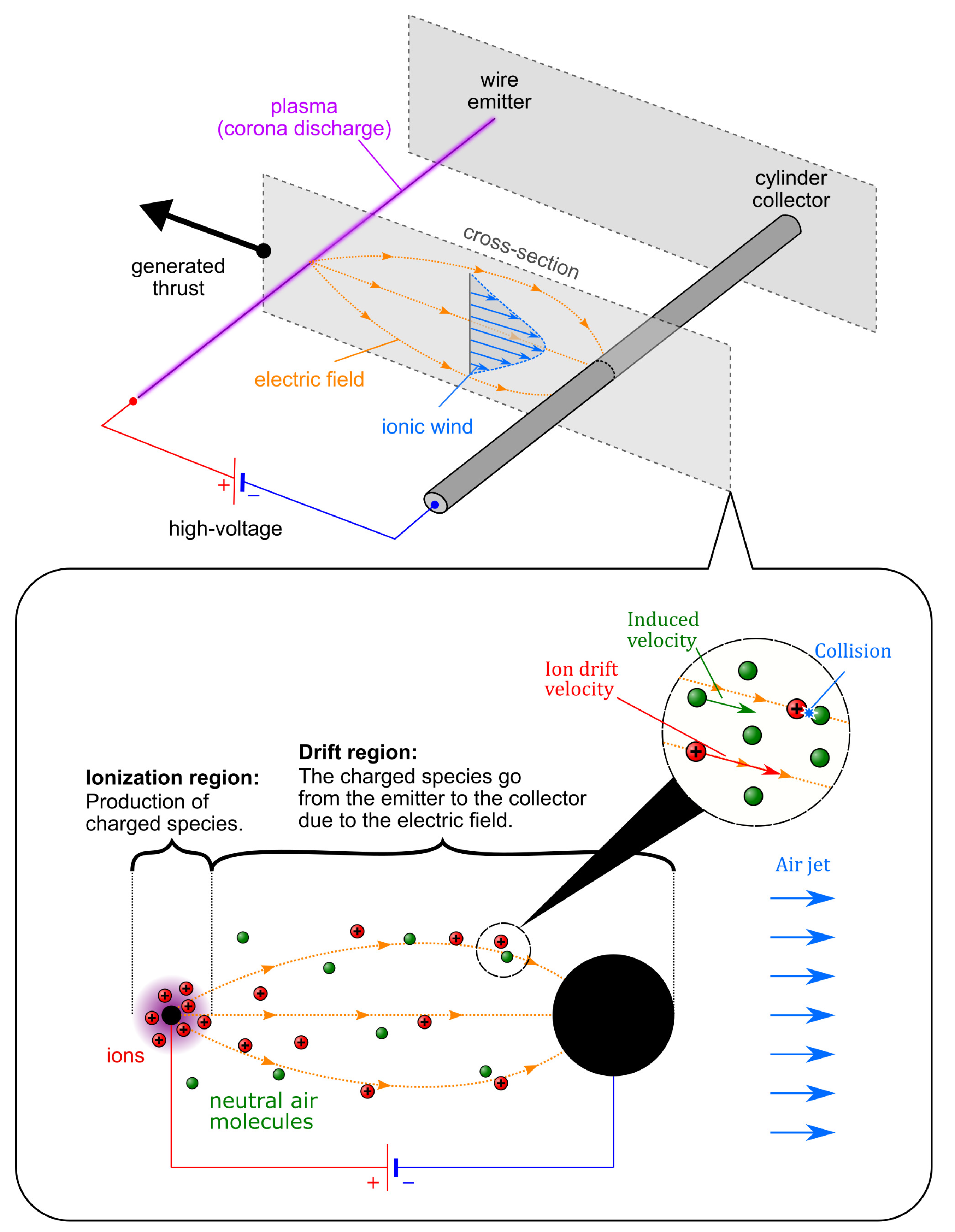
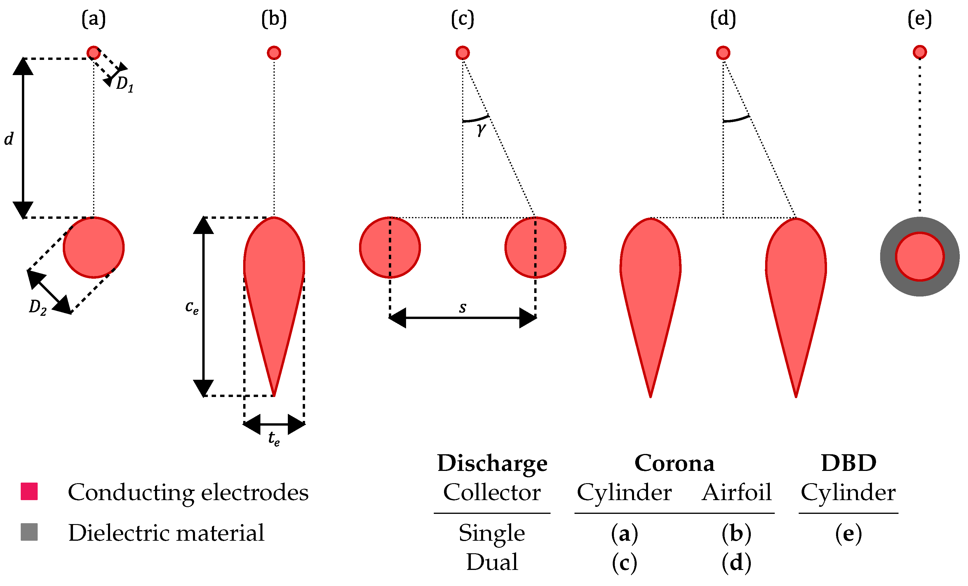
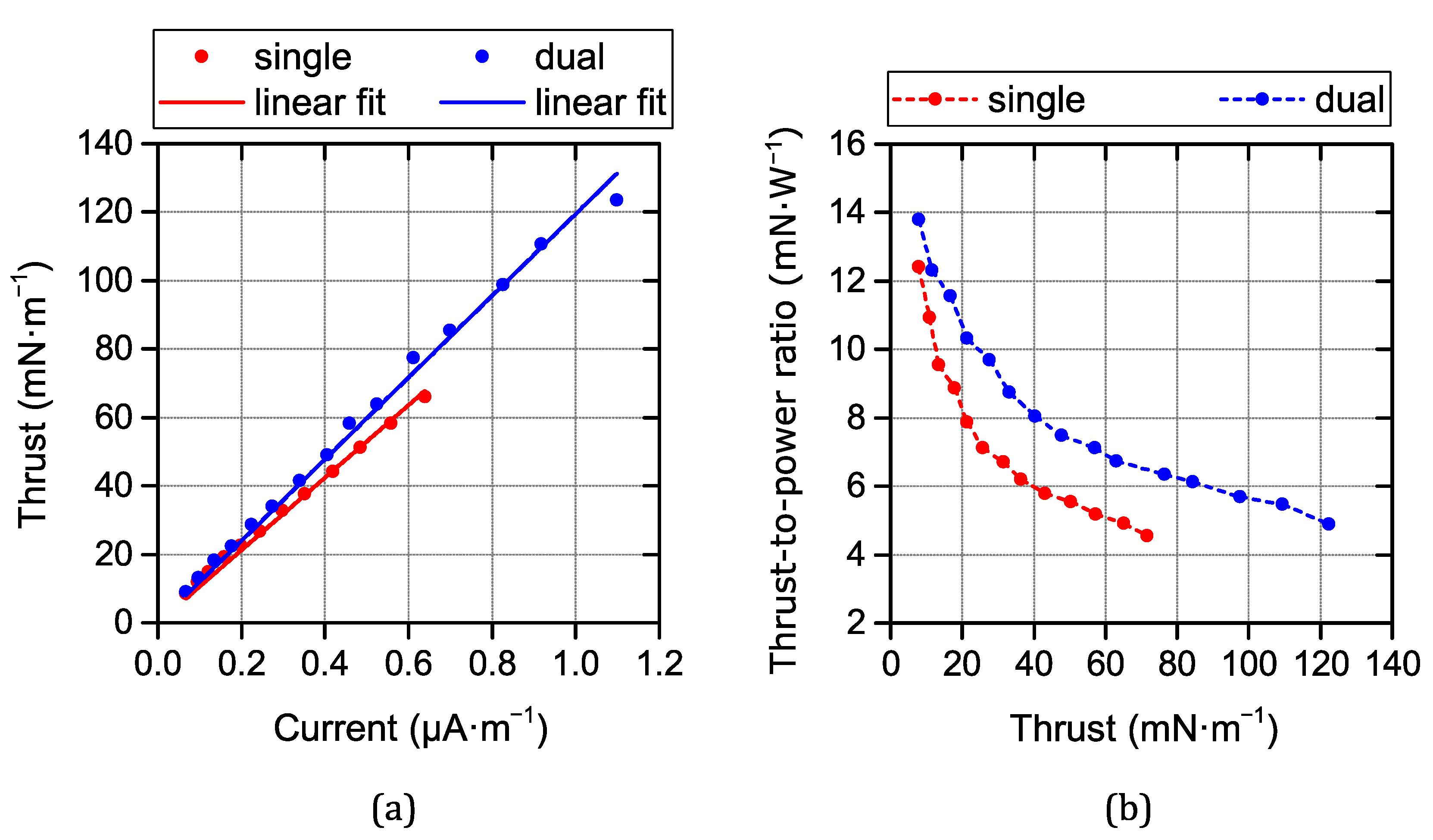
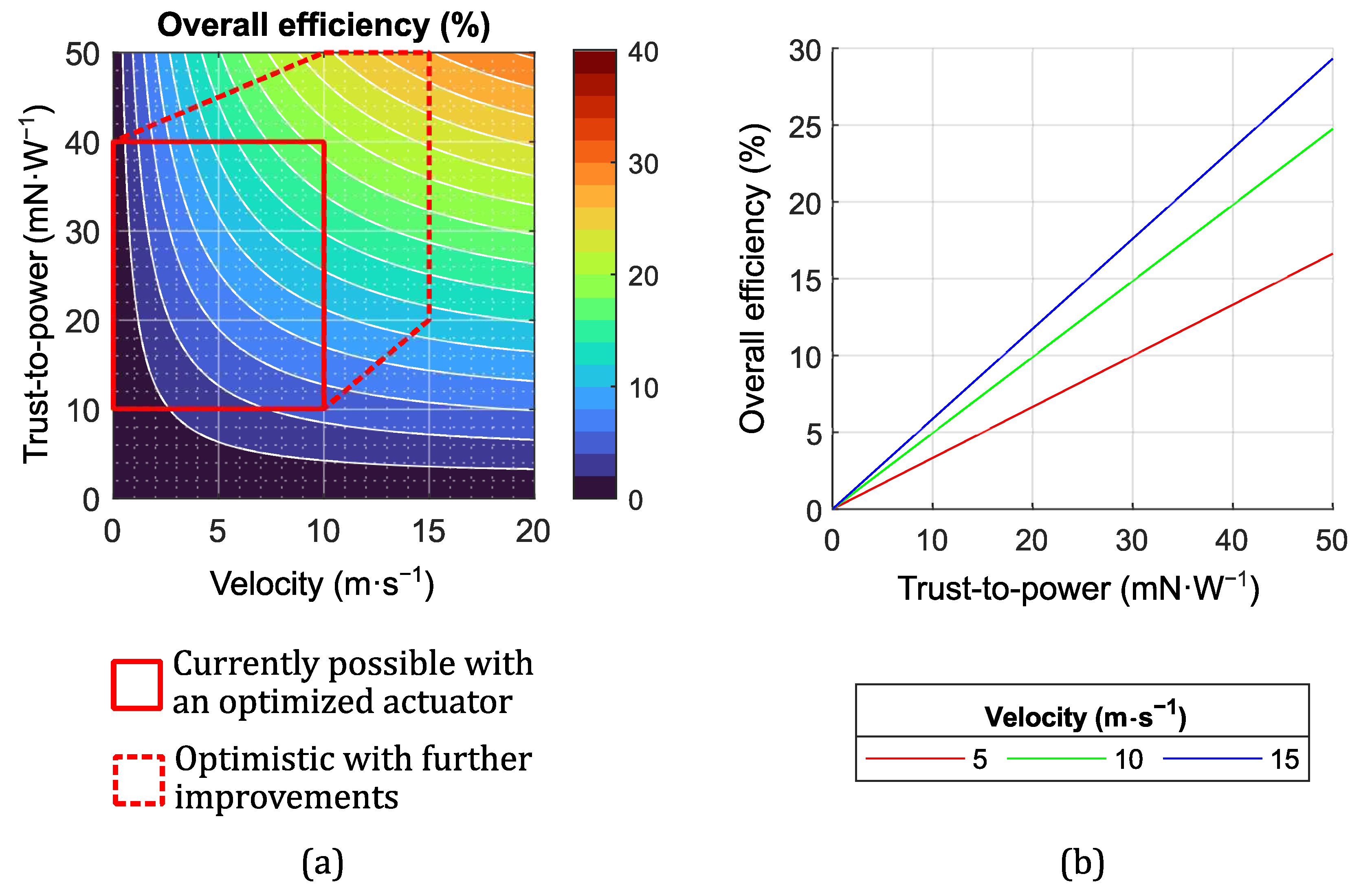
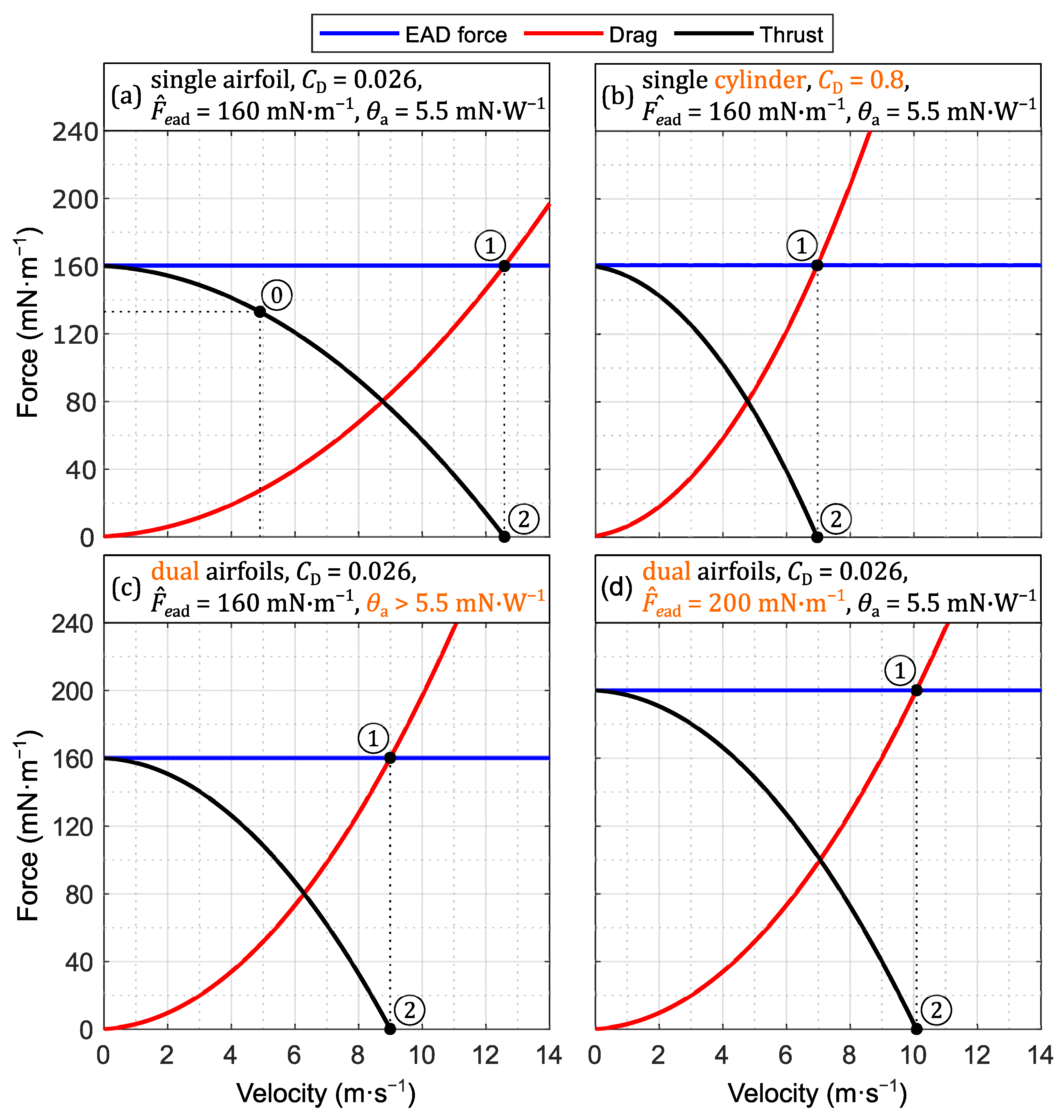
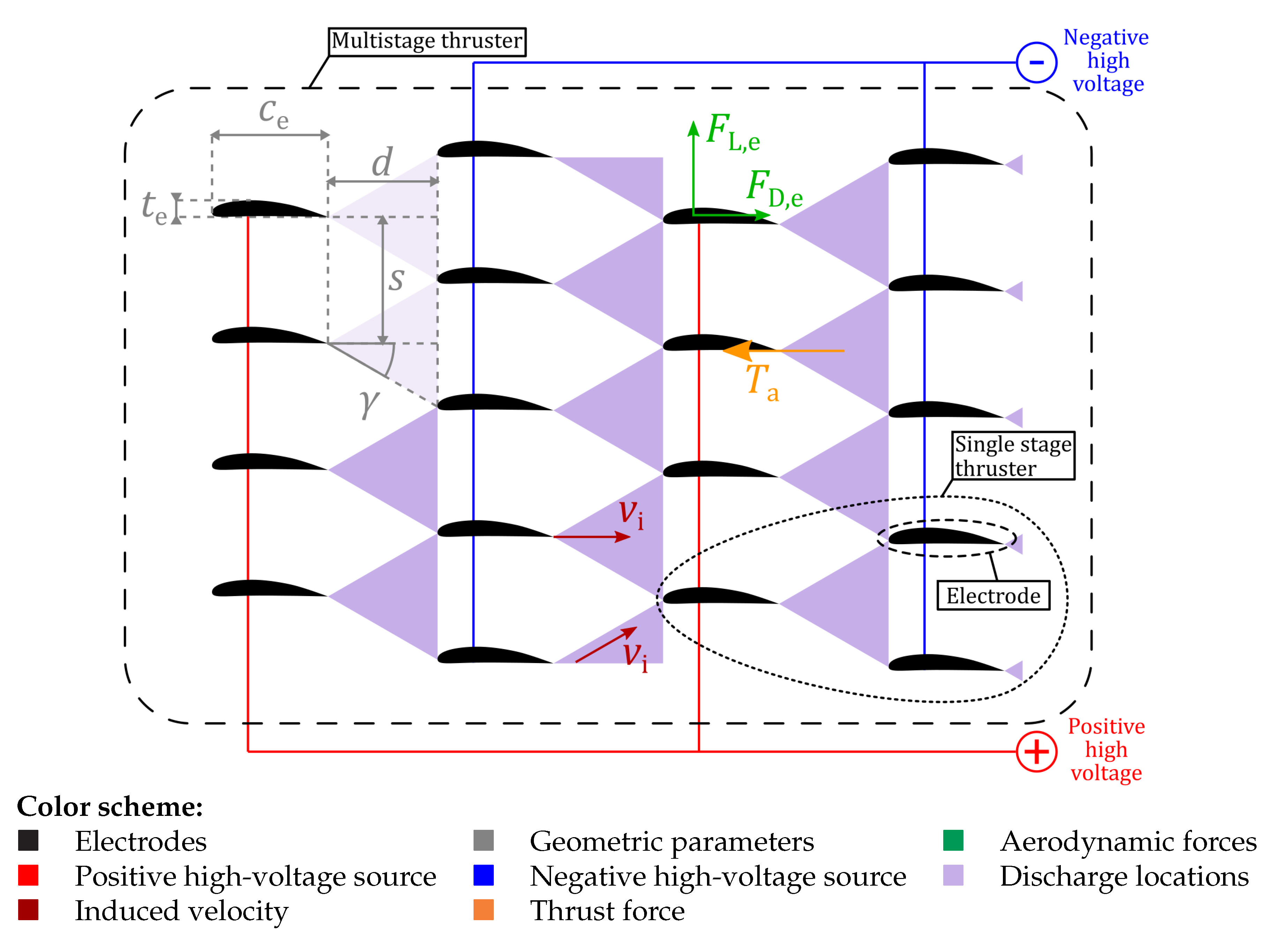
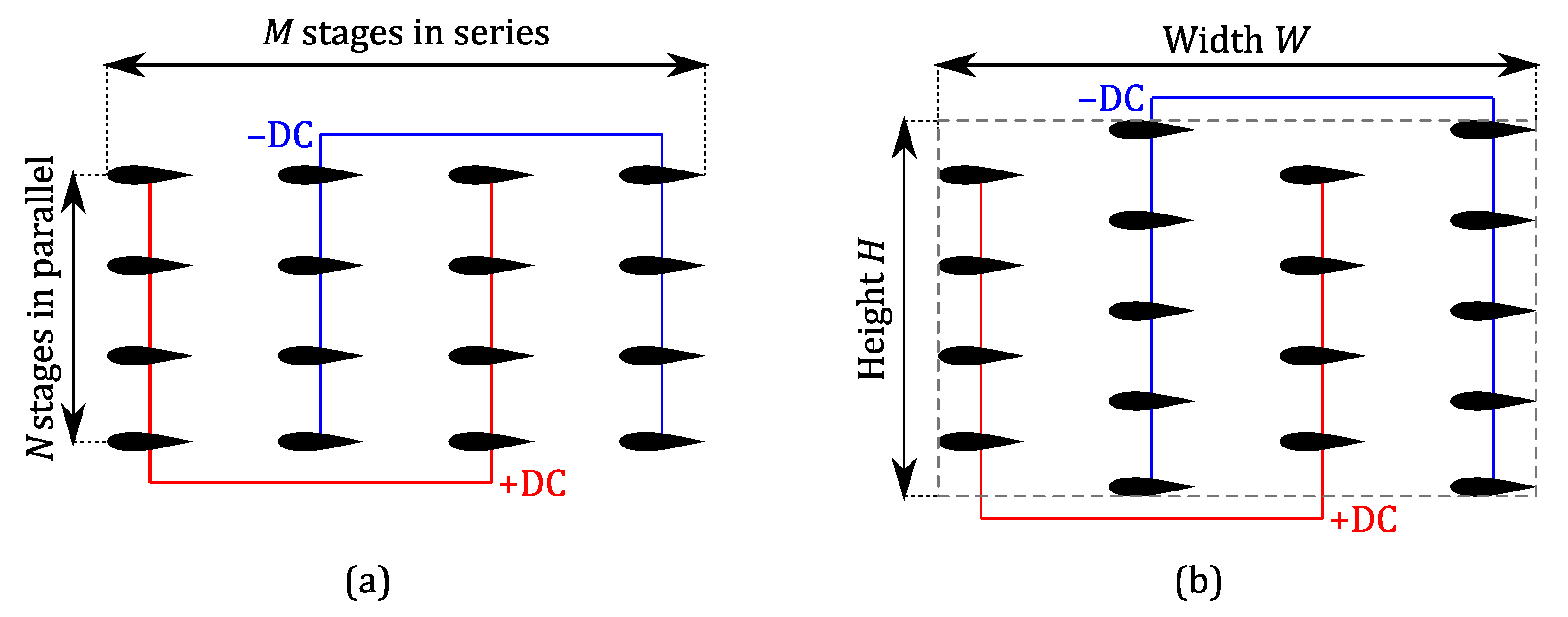
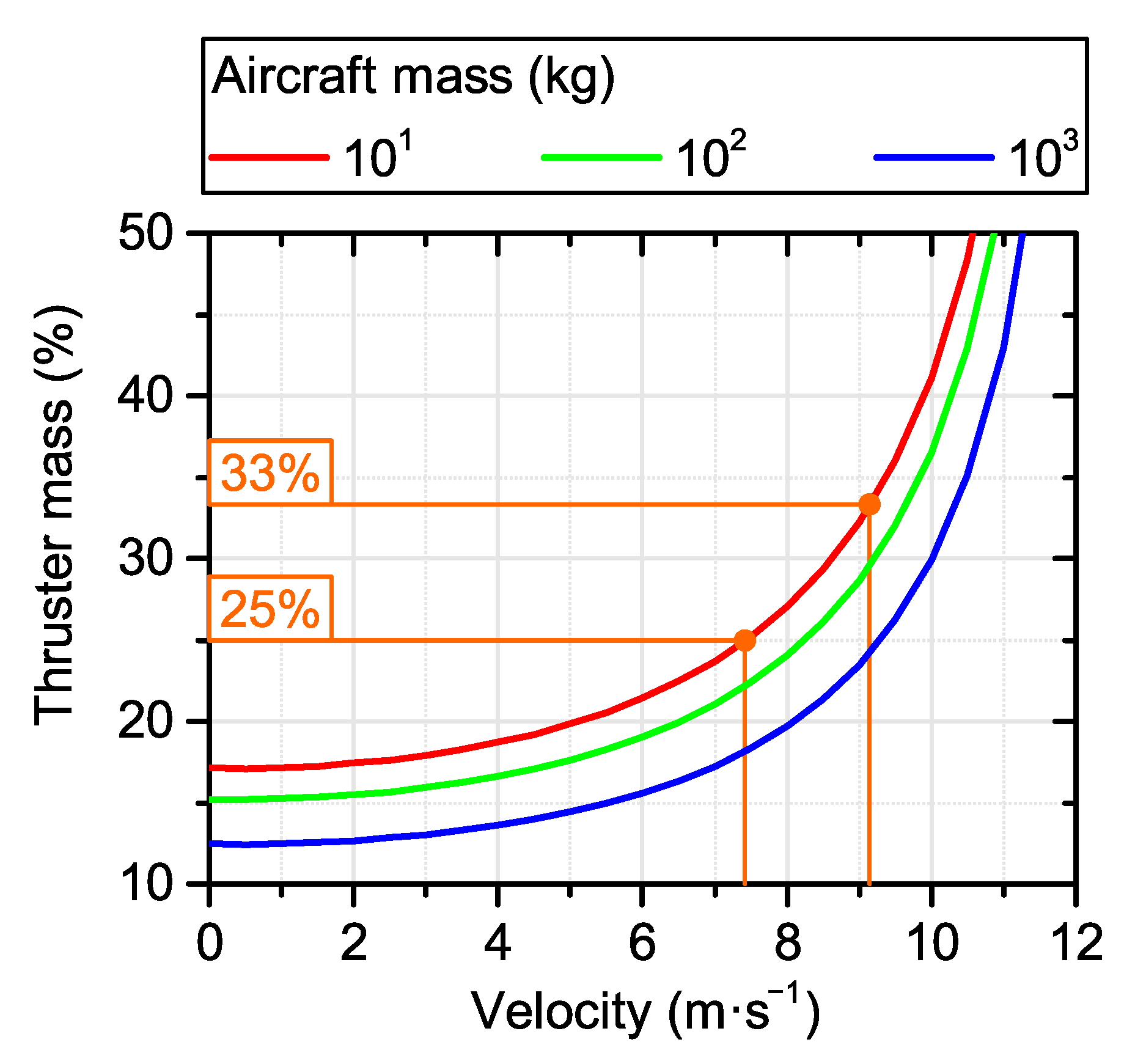
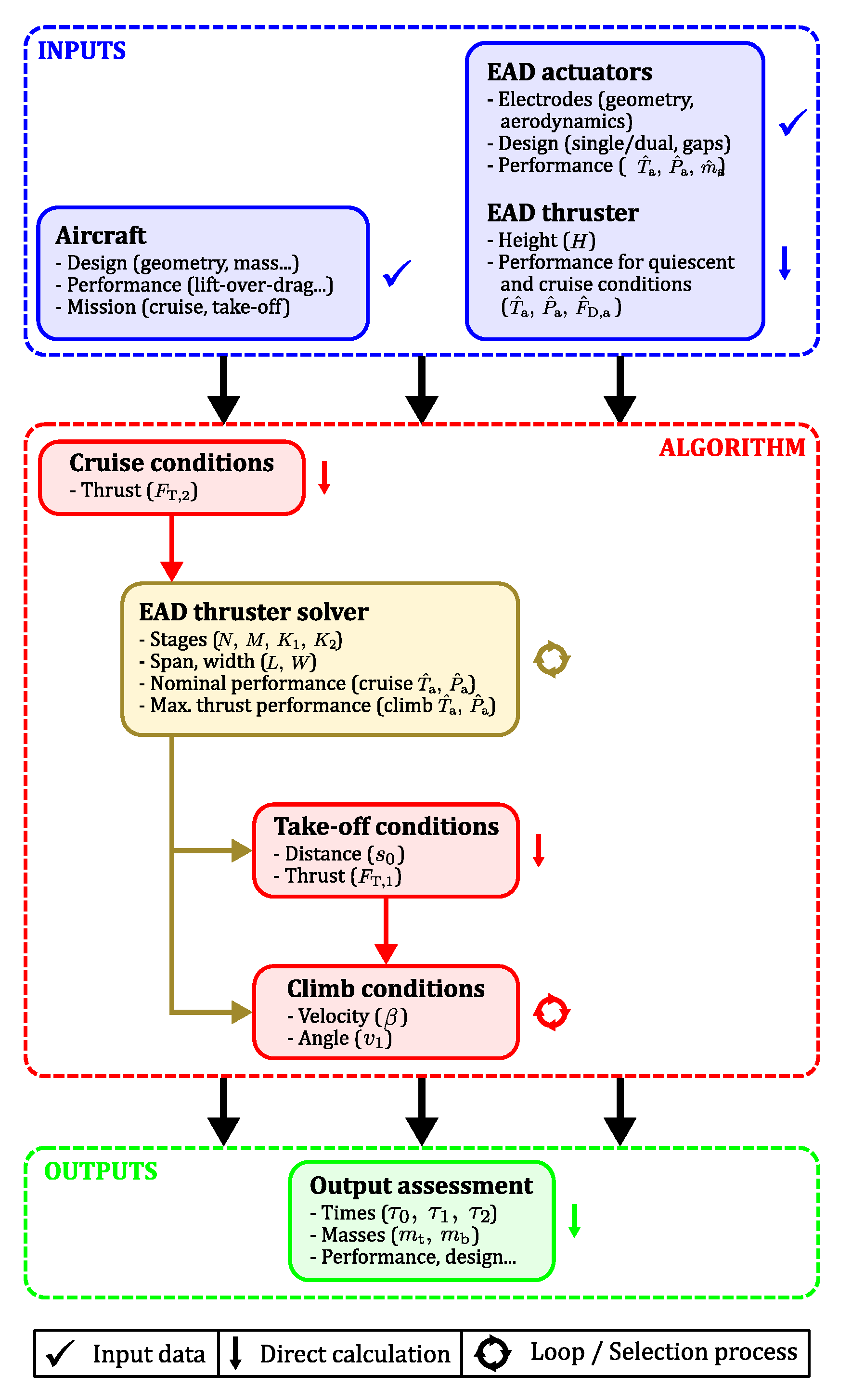
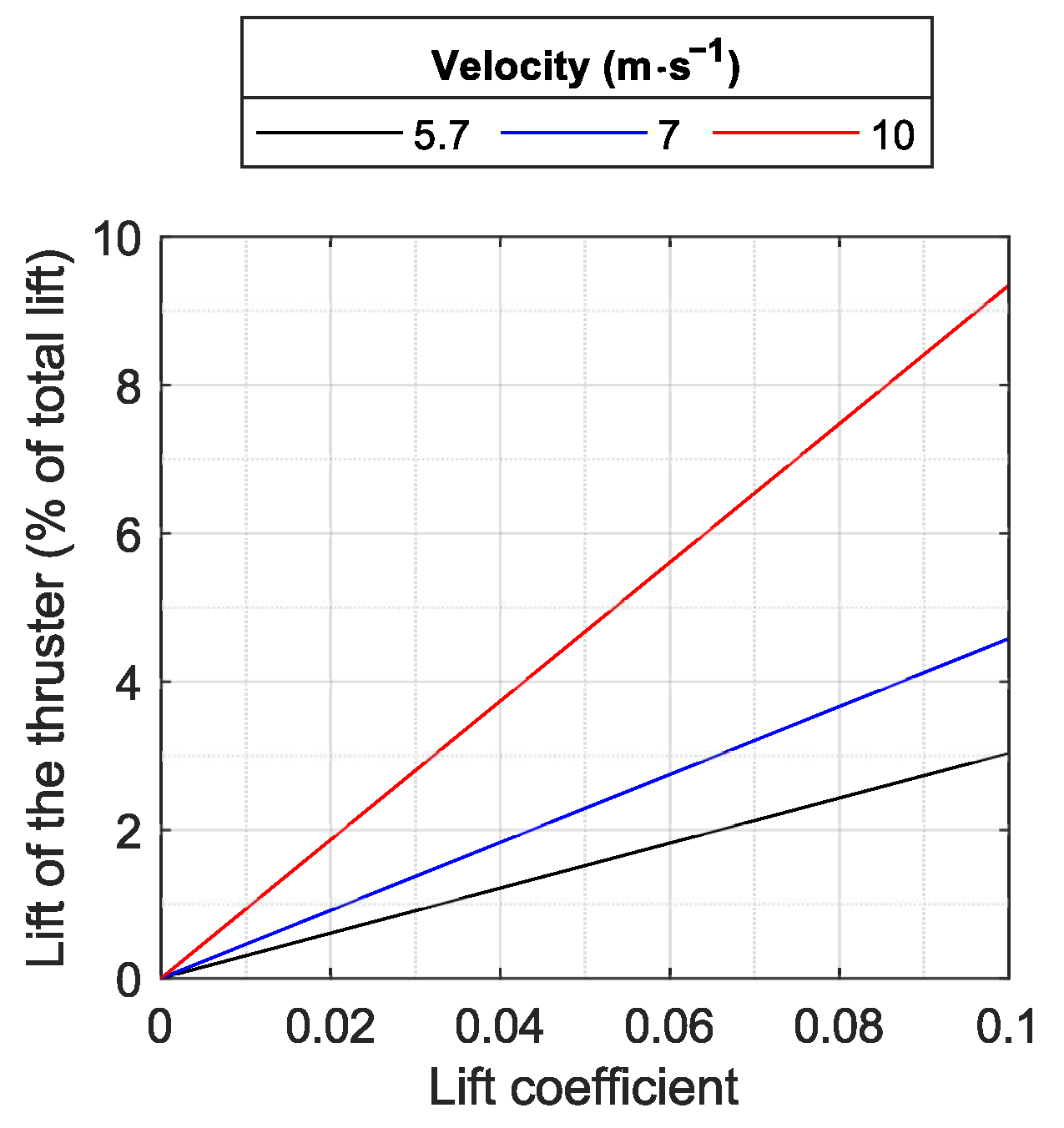
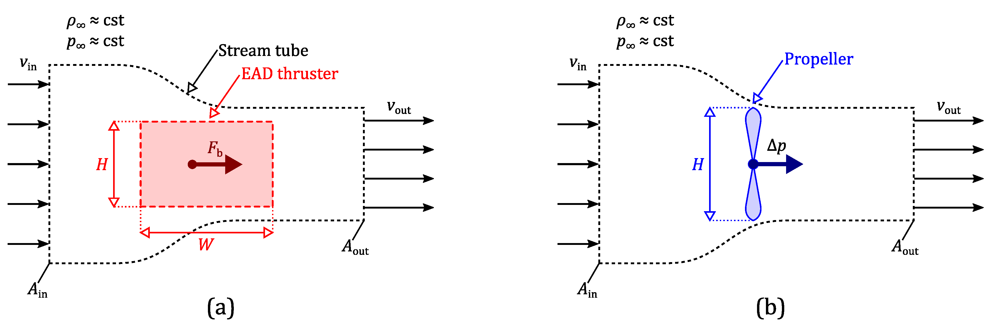
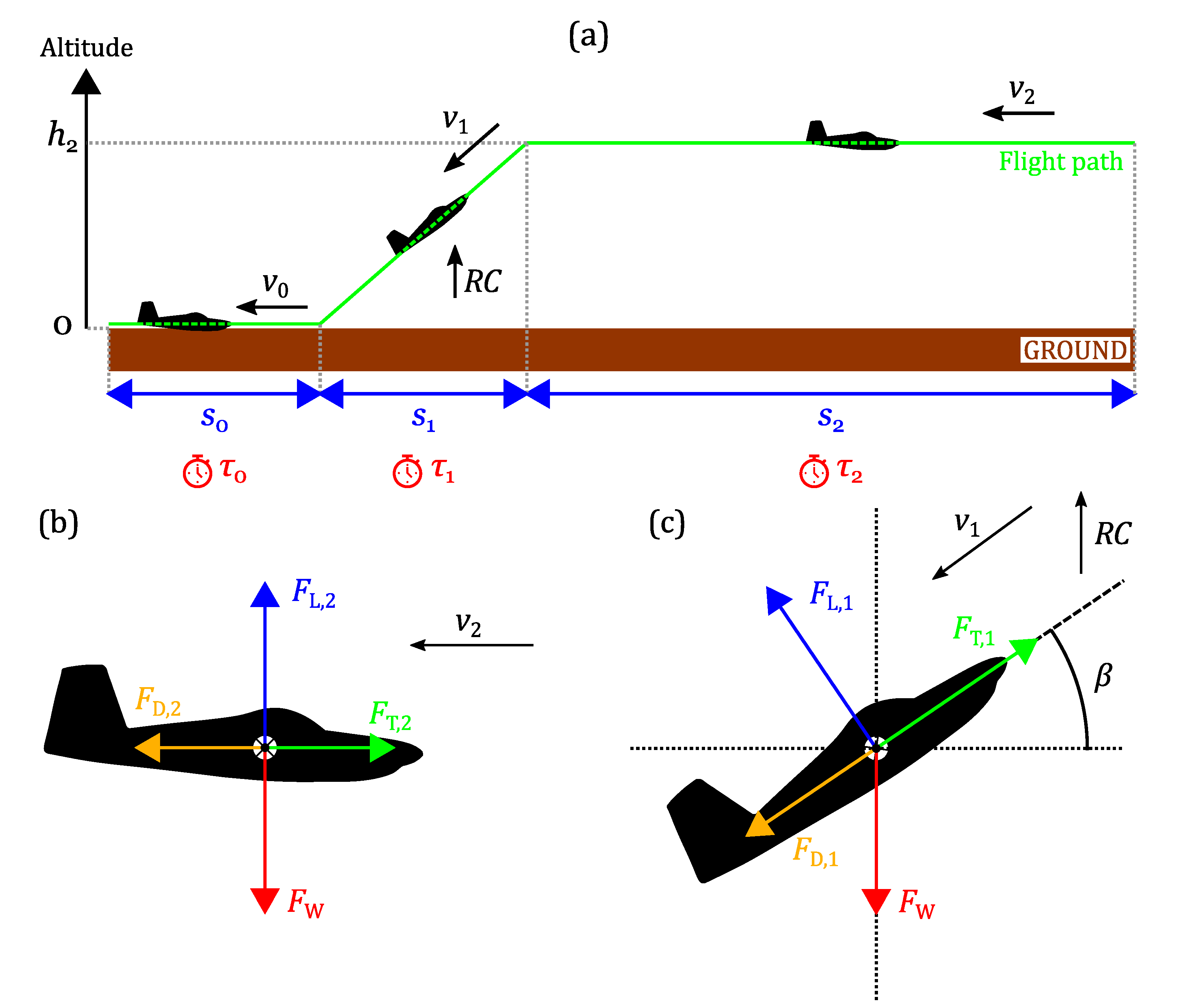
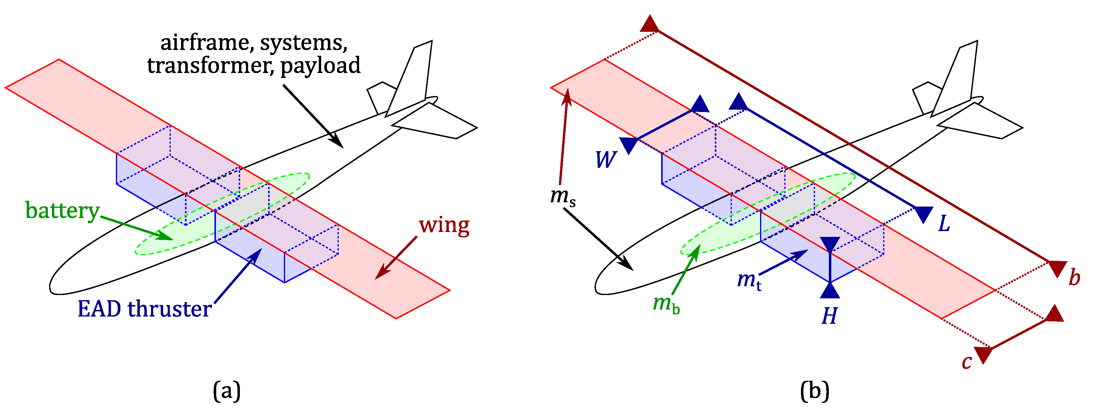
Table 1.
Principal characteristics of the two reference UAVs.
| Aircraft Model: | MIT | Albatross | |||
|---|---|---|---|---|---|
| Aircraft | Mass | (kg) | 2.45 | 10 | |
| Span | b | (m) | 5 | 3 | |
| Aspect ratio | 17.9 | 13.6 | |||
| Lift-over-drag | f | 8 | 28 to 30 | ||
| Battery | Mass | (kg) | 0.23 | 1.2 | |
| Energy density | (Wh) | 130 | 223 | ||
| Mission | Cruise velocity | (m) | 4.8 | 18.9 | |
| Endurance | (h) | - | 4 | ||
| Take-off | Catapulted | Catapulted or 100 m | |||
| Engine | Type | EAD, single collectors | Electric with propeller | ||
| Frontal dimensions | (m) | Diameter of 0.38 | |||
| Mass | (kg) | 0.41 | 0.29 | ||
| Thrust | (mN) | 133 (in cruise) | - | ||
| Power | (W) | 25.8 (in cruise) | - |
Table 2.
Results for EAD-propelled versions of the Albatross UAV (size of the thruster = height × total chord × span).
Table 2.
Results for EAD-propelled versions of the Albatross UAV (size of the thruster = height × total chord × span).
| Aircraft | Albatross UAV (Reference) | EAD-Propelled | ||
|---|---|---|---|---|
| EAD Albatross 1 | EAD Albatross 2 | EAD Albatross 3 | ||
| Thruster size | - | 0.28 × 0.3 × 4.3 | 0.28 × 0.3 × 2.1 | 0.28 × 0.18 × 0.9 |
| Configuration | - | dual | dual | dual |
| Thrust scaling | - | ×1 | ×2 | ×10 |
| Cruise velocity | 18.9 m | 4.5 m | 6.6 m | 18.9 m |
| Endurance | 4 h | 6 min | 42 min | 4 h |
| Ceiling | 120 m | 10 m | 10 m | 120 m |
| Available mass | 8.5 kg | 8.5 kg | 8.5 kg | 8.5 kg |
| Wingspan | 3 m | 4.3 m | 3 m | 3 m |
| Aspect ratio | 13.6 | 19.5 | 13.6 | 13.6 |
Table 3.
Results for EAD-propelled UAVs with a similar take-off mass (10 kg) and lift-over-drag ratio (28) as the Albatross UAV.
Table 3.
Results for EAD-propelled UAVs with a similar take-off mass (10 kg) and lift-over-drag ratio (28) as the Albatross UAV.
| Aircraft | Albatross (Reference) | EAD-Propelled | |||||
|---|---|---|---|---|---|---|---|
| UAV 1 | UAV 2 | UAV 3 | UAV 4 | UAV 5 | UAV 6 | ||
| Thruster size | - | 0.28 × 0.3 × 3.6 | 0.28 × 0.3 × 2.8 | 0.28 × 0.3 × 2.8 | 0.28 × 0.3 × 3.8 | 0.28 × 0.3 × 2.7 | 0.28 × 0.18 × 3.5 |
| Configuration | - | single | dual | dual | dual | dual | dual |
| Thrust scaling | - | ×1.28 | ×1.55 | ×1.55 | ×1.55 | ×3.1 | ×3.1 |
| Cruise velocity | 18.9 m | 4.8 m | 5.7 m | 5.7 m | 4.8 m | 5.7 m | 7.3 m |
| Endurance | 4 h | 46 min | 6 min | 1 h 33 min | 1 h 42 min | 4 h 10 min | 2 h 20 min |
| Ceiling | 120 m | 30 m | 30 m | 30 m | 30 m | 120 m | 30 m |
| Available mass | 8.5 kg | 6.5 kg | 8.5 kg | 6.5 kg | 6.5 kg | 6.5 kg | 6.5 kg |
| Wingspan | 3 m | 5 m | 5 m | 5 m | 5 m | 5 m | 5 m |
| Aspect ratio | 13.6 | 20 | 20 | 20 | 20 | 20 | 20 |
| Conceivable aircraft | Optimistic aircraft | ||||||
Disclaimer/Publisher’s Note: The statements, opinions and data contained in all publications are solely those of the individual author(s) and contributor(s) and not of MDPI and/or the editor(s). MDPI and/or the editor(s) disclaim responsibility for any injury to people or property resulting from any ideas, methods, instructions or products referred to in the content. |
© 2024 by the authors. Licensee MDPI, Basel, Switzerland. This article is an open access article distributed under the terms and conditions of the Creative Commons Attribution (CC BY) license (https://creativecommons.org/licenses/by/4.0/).
Share and Cite
MDPI and ACS Style
Grosse, S.; Moreau, E.; Binder, N. Modeling of the Flight Performance of a Plasma-Propelled Drone: Limitations and Prospects. Drones 2024, 8, 114. https://0-doi-org.brum.beds.ac.uk/10.3390/drones8030114
AMA Style
Grosse S, Moreau E, Binder N. Modeling of the Flight Performance of a Plasma-Propelled Drone: Limitations and Prospects. Drones. 2024; 8(3):114. https://0-doi-org.brum.beds.ac.uk/10.3390/drones8030114
Chicago/Turabian StyleGrosse, Sylvain, Eric Moreau, and Nicolas Binder. 2024. "Modeling of the Flight Performance of a Plasma-Propelled Drone: Limitations and Prospects" Drones 8, no. 3: 114. https://0-doi-org.brum.beds.ac.uk/10.3390/drones8030114