Research on A Global Path-Planning Algorithm for Unmanned Arial Vehicle Swarm in Three-Dimensional Space Based on Theta*–Artificial Potential Field Method

Abstract

The current challenge in drone swarm technology is three-dimensional path planning and adaptive formation changes. The traditional A* algorithm has limitations, such as low efficiency, difficulty in handling obstacles, and numerous turning points, which make it unsuitable for complex three-dimensional environments. Additionally, the robustness of drone formations under the leader–follower mode is low, and effectively handling obstacles within the environment is challenging. To address these issues, this study proposes a virtual leader mode for drone formation flight and introduces a new Theta*–APF method for three-dimensional space drone swarm path planning. This algorithm optimizes the A* algorithm by transforming it into an omnidirectional forward Theta* algorithm. It also enhances the heuristic function by incorporating artificial potential field methods in a three-dimensional environment. Formation organization and control of UAVs is achieved using speed-control modes. Compared to the conventional A* algorithm, the Theta*–APF algorithm reduces the search time by about 60% and the trip length by 10%, in addition to the safer flight of the UAV formation, which is subject to artificial potential field repulsion by about 42%.

1. Introduction

Currently, single UAVs are widely used in industrial production, logistics transportation, and other fields. In comparison to single-UAV systems, multi-UAV systems operating in formation can significantly enhance the flexibility of individual UAVs and greatly compensate for their limitations [1,2]. At the same time, the diversity of UAV mission environments poses challenges for safe flights in complex 3D spaces. An excellent path-planning algorithm can guide UAVs to reach their designated locations safely and quickly, thereby improving mission efficiency. Several algorithms, such as the artificial potential field method, the dynamic window method, the random trees algorithm, and the Dijkstra algorithm, etc. [3,4,5,6,7,8,9], have been applied in 2D path planning. Based on the existing related 2D path-planning algorithms, the development of a path-planning algorithm that can meet the needs of UAV formations to navigate in 3D environments will be able to be of great practical significance in the execution of UAV formation missions, such as performances, disaster relief, exploration, and so on.

The key technology for multi-UAVs formation flight lies in various control algorithms, including the flight-control algorithm for each individual UAV within the formation, the local path-planning algorithm, and the information communication and formation-control algorithm among multiple UAVs. Multi-UAV systems can bring numerous advantages by operating in formation. During the execution of multi-UAV missions, UAVs must possess good obstacle perception and avoidance capabilities due to the complexity and uncertainty of the surrounding environment. It is necessary to coordinate the trajectories of a single UAV and multiple UAVs to ensure that obstacles are avoided while handling the scheduled tasks. In the field of multi-UAVs formation flight and path navigation, numerous scholars have conducted extensive research [2,10,11,12,13,14,15,16,17,18,19,20,21]. Among them, Shao et al. [2] proposed an improved particle swarm optimization (PSO) algorithm that enhances the speed and optimality of path planning. They achieve this by accelerating the convergence rate of the algorithm through a strategy. Pan et al. [12] proposed an improved artificial potential field method for UAV formation path planning and adopted a leader–follower mode to ensure that the following UAV maintains the desired angle and distance. Liu et al. [13] proposed an improved RRT* formation path-planning algorithm that optimizes the speed of UAV formation in complex environments. Hoang et al. [14] proposed an angle-encoded particle swarm optimization (θ-PSO) algorithm that accelerates the convergence of the particle swarm and confirmed its validity and feasibility in formation path planning. Chen H et al. [15] improved the traditional artificial potential field method for path planning by introducing a local minimum value judgment mechanism to break out of local minimum values. Chen Q et al. [16] proposed a trajectory-planning method that fuses Dubins trajectory with particle swarm optimization (PSO), generating feasible trajectories in real time during formation transformations. Wu et al. [17] proposed a method to calculate the collision probability of drones while considering task space and UAV number constraints, implementing automatic tracking and prediction of UAV cluster trajectories to prevent path conflicts in clusters. Carlos et al. from the University of Toronto [18] implemented a multi-UAV trajectory-planning and obstacle-avoidance algorithm based on DMPC distributed model predictive control, utilizing “on-demand control” to optimize the scalability of the system; this significantly reduces the computational time compared to traditional algorithms. Palossi et al. [19] achieved parallel real-time path planning for UAVs using the Dijkstra algorithm through a parallel algorithm of UAV real-time path planning. Yao J et al. [20] enhanced the A* algorithm by reducing the search time and search compensation, enabling it to avoid specific obstacles. Zhang et al. [21] introduced the branch-selection fast-exploration random tree (BS-RRT) algorithm to address the issue of UAV path planning in narrow urban channels.

Currently, common path-planning algorithms include the artificial potential field method, the dynamic window method, the random number algorithm, Dijkstra’s algorithm, etc. However, these algorithms all have some drawbacks. Due to the three-dimensional (3D) nature of UAV flight, the applicability of these algorithms is still relatively limited. For instance, the artificial potential field method frequently fails to identify the optimal path when the gravitational force is too weak, and it readily becomes trapped in local optima when the gravitational force is too strong, resulting in increased performance overheads [22], p. 2. The dynamic window method also faces the problem of being prone to falling into local optima [23], pp. 1–2. The Dijkstra algorithm suffers from significant performance overheads and cannot be executed in a 3D environment [24], p. 1. The A* algorithm, which is an improvement on the Dijkstra algorithm, often fails to plan the optimal path due to limited movement directions [25], p. 1. In addition, current research on path planning often simplifies the flight environment, and the flight scenarios do not accurately represent the complex situations found in both indoor and outdoor environments. As a result, there is a significant discrepancy between the simulation results and the actual conditions. Some studies do not take into account the 3D flight characteristics of UAVs, and their path planning is limited to two dimensions. Some algorithms also lack sufficient obstacle avoidance processing for obstacles in the environment, which makes it challenging for UAVs to navigate around them [26].

There are several organizational models for drone formations, including the leader–follower mode and the virtual pilot mode. The leader–follower mode was first proposed by Desai J P [27] and is a widely used algorithm, but the model relies too much on the navigator and is difficult to deal with navigator crashes and lacks sufficient robustness. Weitzenfeld A et al. [28] proposed an algorithm with a backup navigator to improve the leader–follower model’s robustness. Lewis M A [29] et al. proposed the virtual navigator concept, in which there is no real navigating UAV, but a virtual navigator instead, which further improves the stability compared to the leader–follower model.

To address the aforementioned issues, this paper proposes a path-planning algorithm called the Theta*–APF method. Compared to the traditional A* algorithm [30], this algorithm reduces the path search time by approximately 60% and the total length of the planned path by approximately 10%. The algorithm also works well in environments with complex obstacles, such as indoors where various objects are placed, between urban complexes, etc. In addition, we utilize the virtual leader–follower model to coordinate the formation flight of drones. We combine this model with a global artificial potential field method to enable local obstacle avoidance for the drone formation.

2. Theta*–Artificial Potential Field Method Path-Planning Algorithm

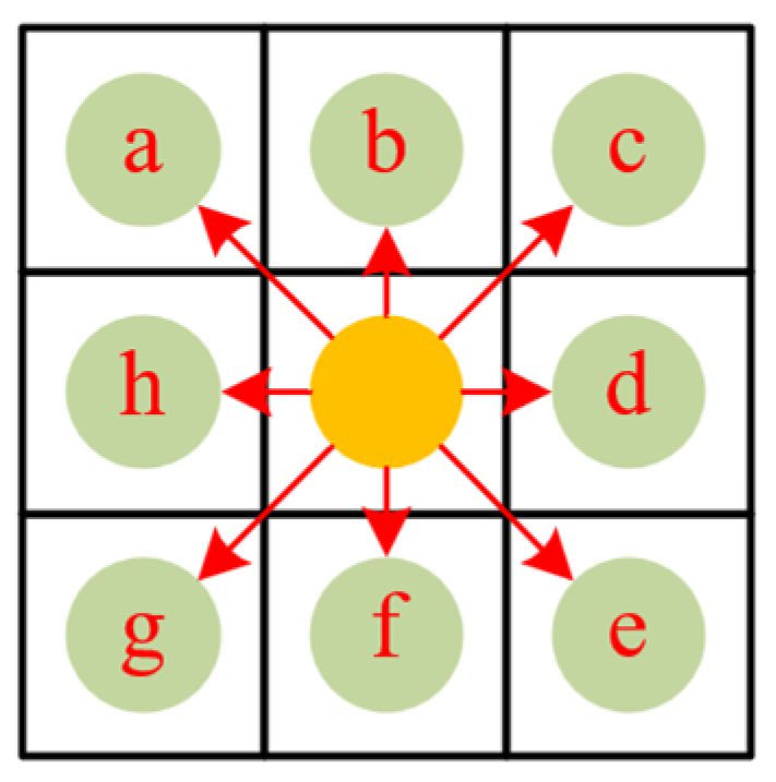
2.1. A* Algorithm

As a heuristic search algorithm, the A* algorithm combines the advantages of Dijkstra’s algorithm with the greedy algorithm strategy [31]. It is commonly used for solving point-to-point optimal path-planning problems in known static maps. The A* algorithm performs path planning in grid maps by starting from the initial node and expanding outward step by step. At each expansion, it uses an evaluation function to calculate the total movement cost of the newly searched nodes and selects the node with the lowest movement cost for the next expansion. The A* algorithm continuously selects new nodes for expansion and iterates until the destination node is reached. The core of the algorithm is the evaluation function, as shown in Equation (1).

$$f\left(n\right)=g\left(n\right)+h\left(n\right),$$

(1)

In the above equation, $g\left(n\right)$ denotes the cost of moving from the starting point to the current node. It refers to the length of the path from the starting point to the current node. $h\left(n\right)$ denotes the expected cost from the current node to the end point, i.e., it is the heuristic function of the A* algorithm. $f\left(n\right)$ denotes the integrated cost of the current node’s movement, i.e., it is the integrated priority of the next move.

The choice of the heuristic function $h\left(n\right)$ in the A* algorithm is especially critical as it can control the search speed and accuracy of the algorithm. The smaller the value of $h\left(n\right)$, the more nodes are searched by the A* algorithm, making it easier to select the globally optimal path but slowing down the search speed. On the other hand, a larger value of $h\left(n\right)$ results in fewer nodes being searched by the A* algorithm, making the search faster but increasing the risk of falling into a local optimal path. When the value of $h\left(n\right)$ is 0, the A* algorithm no longer utilizes the heuristic function, and instead degrades to the Dijkstra algorithm. If the value of $h\left(n\right)$ is much larger than the value of $g\left(n\right)$, at this time, the role of $g\left(n\right)$ will be ignored. The A* algorithm’s search speed is greatly improved, but it may not be able to find the optimal path. It is generally recognized that, when $g\left(n\right)$ and $h\left(n\right)$ are equal, the A* algorithm will be able to find the optimal path without any additional node searches, making the search time relatively efficient.

The most commonly used methods for calculating the main heuristic function are Manhattan distance calculation, Euclidean distance, and Chebyshev distance. In these methods, the current node is set as $({\mathrm{x}}_{\mathrm{n}},{\mathrm{y}}_{\mathrm{n}})$ and the end point is set as $({\mathrm{x}}_{\mathrm{e}},{\mathrm{y}}_{\mathrm{e}})$.

2.1.1. Manhattan Distance

Manhattan distance is the sum of the horizontal and vertical distances between two points. The formula for Manhattan distance is shown in Equation (2).

$$\mathrm{h}\left(\mathrm{x}\right)=\left|{\mathrm{x}}_{\mathrm{n}}-{\mathrm{x}}_{\mathrm{e}}\right|+\left|{\mathrm{y}}_{\mathrm{n}}-{\mathrm{y}}_{\mathrm{e}}\right| ,$$

(2)

2.1.2. Euclidean Distance

The Euclidean distance is the straight-line distance between two points, as shown in Equation (3).

$$\mathrm{h}(\mathrm{x})=\sqrt{{\left({\mathrm{x}}_{\mathrm{n}}-{\mathrm{x}}_{\mathrm{e}}\right)}^2+{\left({\mathrm{y}}_{\mathrm{n}}-{\mathrm{y}}_{\mathrm{e}}\right)}^2} ,$$

(3)

2.1.3. Chebyshev Distance

The Chebyshev distance is defined as the maximum absolute difference between the coordinates of two points on the x and y axes, as represented by Equation (4).

$$\mathrm{h}\left(\mathrm{x}\right)=\mathrm{m}\mathrm{a}\mathrm{x}\left\{\left|{\mathrm{x}}_{\mathrm{n}}-{\mathrm{x}}_{\mathrm{e}}\right|,\left|{\mathrm{y}}_{\mathrm{n}}-{\mathrm{y}}_{\mathrm{e}}\right|\right\} ,$$

(4)

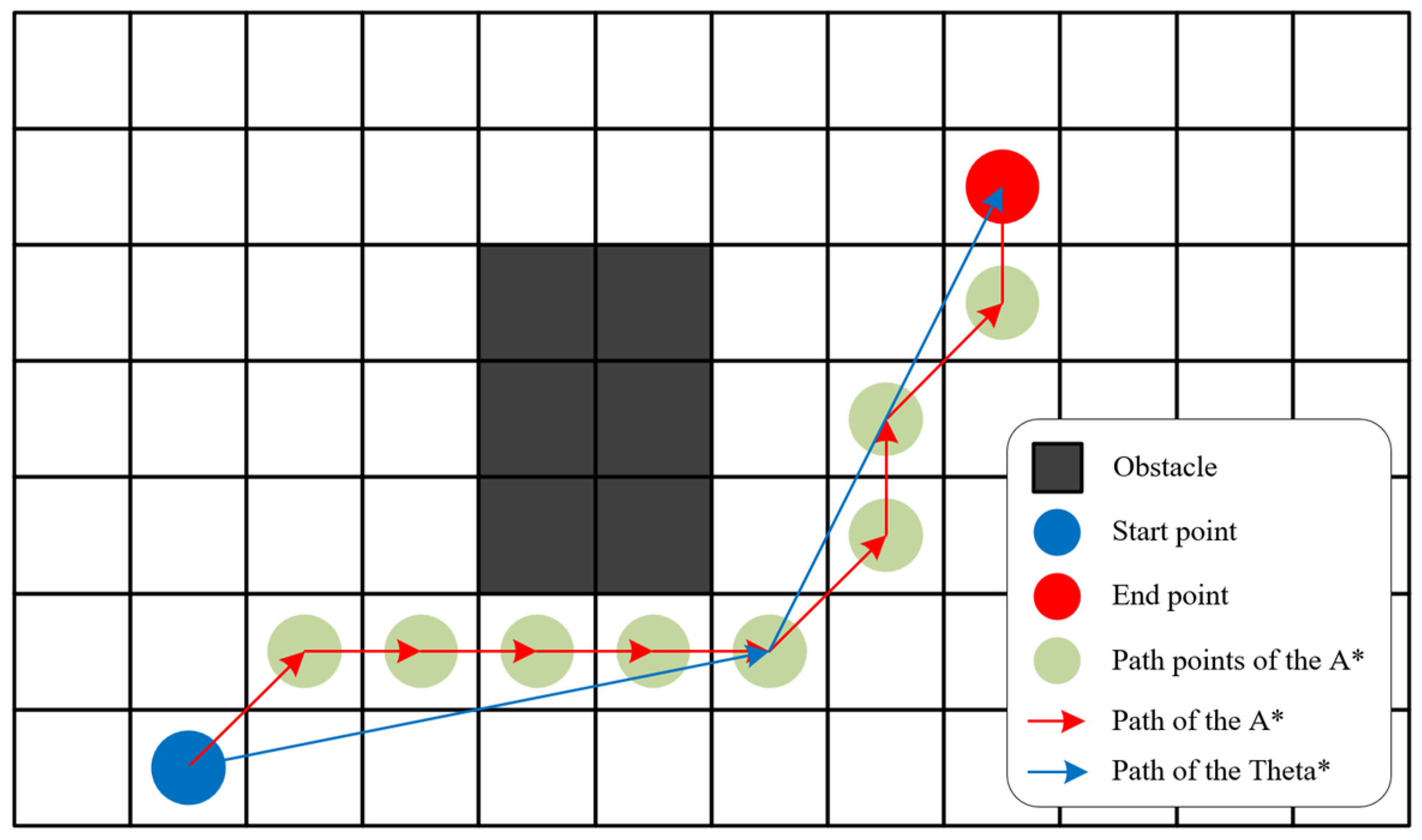
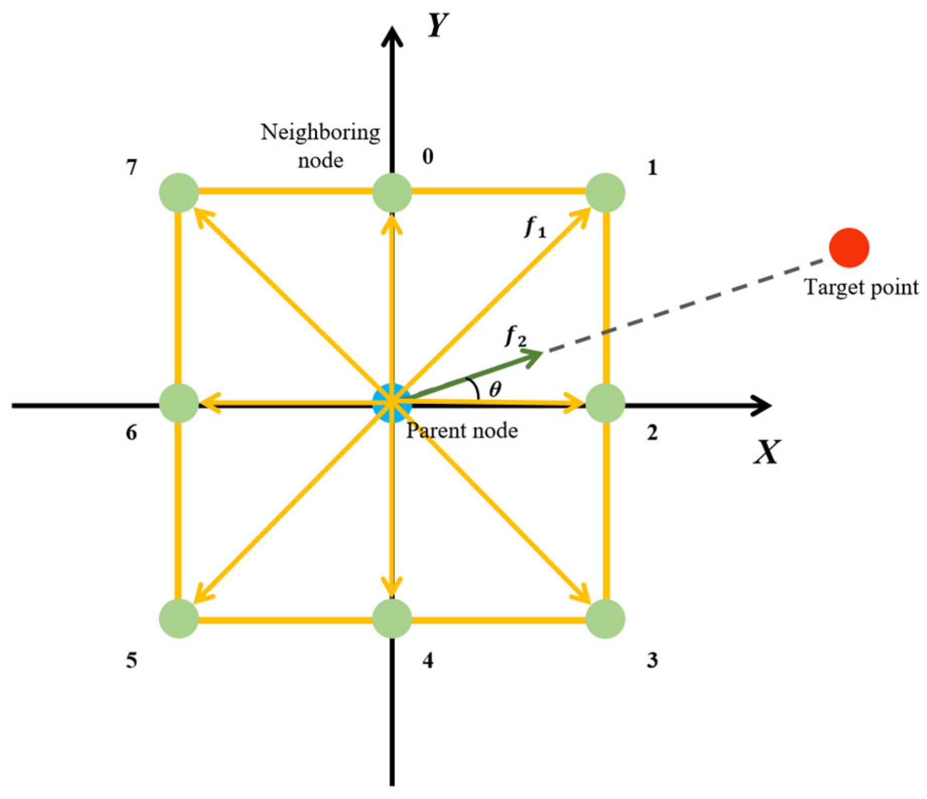
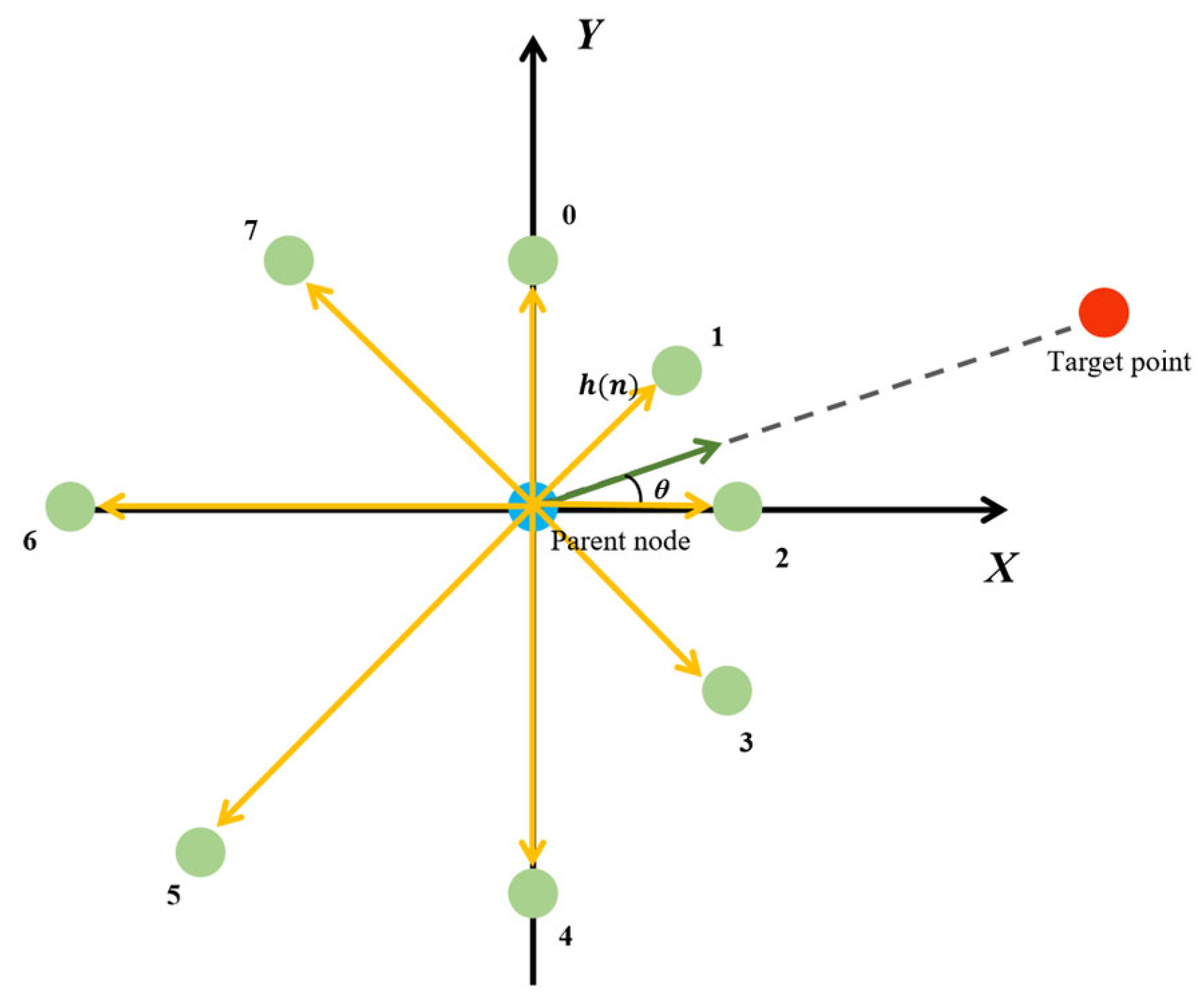
2.2. Theta* Algorithm

The traditional A* algorithm can only move between neighboring nodes each time. It can only move one cell at a time with eight fixed directions: a~h. This algorithm uses the 8-neighborhood search method, as shown in Figure 1. The traditional 8-neighborhood search method restricts the robot’s moving distance and direction, which does not reflect the reality that the robot can move any distance in any direction. Therefore, the optimal path found by the traditional A* algorithm can often be further optimized to achieve a better distance. Therefore, the A* algorithm is extended to optimize it into an omnidirectional A* algorithm. This algorithm can advance any distance in any direction using reverse reasoning. At this point, the A* algorithm evolves into the Theta* algorithm [32]. The advancement of the robot is no longer limited by angle and distance, as shown in Figure 2. The path of the Theta* algorithm is significantly better compared to the A* algorithm, which reduces the redundant turning points in the path of the A* algorithm and reduces the length of the journey.

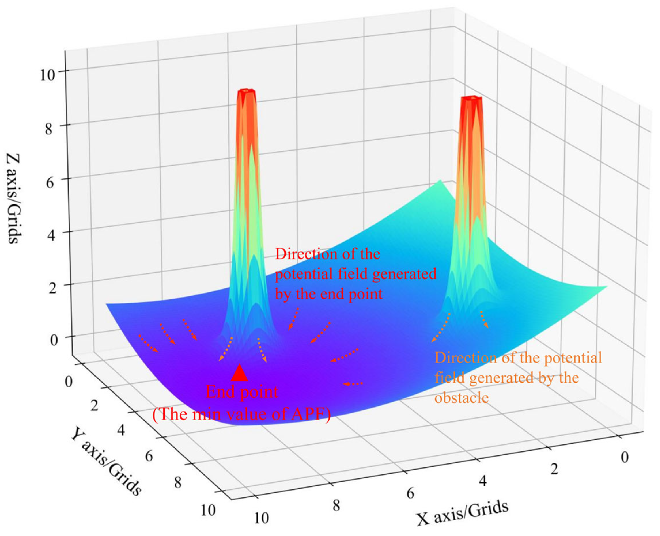
2.3. Heuristic Functions for the Artificial Potential Field Method

The artificial potential field method was proposed by Khatib in [18]. The basic idea is to artificially introduce a virtual potential field into the environment. In path-planning problems, as depicted in Figure 3, the destination is located at the lowest point of the potential field, while obstacles are situated at the highest points. The strength of the potential field for other points in the environment gradually increases as the distance from the destination decreases.

At any given point within the artificial potential field, the robot experiences both the gravitational force exerted by the endpoint and the repulsive force exerted by the obstacle. As the robot moves closer to the endpoint, the gravitational force decreases, while the repulsive force increases as the robot moves closer to the obstacle. Eventually, under the combined influence of gravitational force and repulsive force, the robot moves forward spontaneously, avoiding obstacles, reaching the endpoint. The forces on the robot are shown in Figure 4.

The strength of the potential field at the robot’s location is represented by Equation (5), and it is influenced by a combined force as depicted in Equation (6).

$$\mathrm{U}={\mathrm{U}}_{\mathrm{a}\mathrm{t}\mathrm{t}}+{\mathrm{U}}_{\mathrm{r}\mathrm{e}\mathrm{p}} ,$$

(5)

$$\mathrm{F}={\mathrm{F}}_{\mathrm{a}\mathrm{t}\mathrm{t}}+{\mathrm{F}}_{\mathrm{r}\mathrm{e}\mathrm{p}} ,$$

(6)

where $\mathrm{U}$ is the potential field at the current position of the robot. ${\mathrm{U}}_{\mathrm{a}\mathrm{t}\mathrm{t}}$ represents the gravitational potential field at the current position, while ${\mathrm{U}}_{\mathrm{r}\mathrm{e}\mathrm{p}}$ represents the repulsive potential field at the current position. $\mathrm{F}$ is the total force on the current robot, ${\mathrm{F}}_{\mathrm{a}\mathrm{t}\mathrm{t}}$ represents the gravitational force acting on the robot, and ${\mathrm{F}}_{\mathrm{r}\mathrm{e}\mathrm{p}}$ denotes the repulsive force acting on the robot. The gravitational potential field ${\mathrm{U}}_{\mathrm{a}\mathrm{t}\mathrm{t}}$ at the current position is determined by the distance between the robot’s current position and the endpoint, as illustrated in Equation (7).

$${\mathrm{U}}_{\mathrm{att}}=\frac{1}{2}\lambda {({\mathrm{X}}_{\mathrm{i}}-\mathrm{X})}^2 ,$$

(7)

where $\lambda$ is the gravitational field constant, and ${\mathrm{X}}_{\mathrm{i}}$ and $\mathrm{X}$ are the robot’s current position vector and desired position vector, respectively. The gravitational force ${\mathrm{F}}_{\mathrm{a}\mathrm{t}\mathrm{t}}$, is the negative derivative of ${\mathrm{U}}_{\mathrm{a}\mathrm{t}\mathrm{t}}$, as shown in Equation (8). As the robot approaches the end point, the gravitational force it receives becomes smaller.

$${\mathrm{F}}_{\mathrm{a}\mathrm{t}\mathrm{t}}=-\mathrm{g}\mathrm{r}\mathrm{a}\mathrm{d}\left({\mathrm{U}}_{\mathrm{a}\mathrm{t}\mathrm{t}}\right)=\lambda (\mathrm{X}-{\mathrm{X}}_{\mathrm{i}}) ,$$

(8)

The robot’s current position repulsive force field ${\mathrm{U}}_{\mathrm{r}\mathrm{e}\mathrm{p}}$, is the sum of the repulsive force fields ${\mathrm{U}}_{\mathrm{r}\mathrm{e}\mathrm{p}}^{\mathrm{i}}$, generated by any obstacle at the robot’s current position, as shown in Equation (9). ${\mathrm{U}}_{\mathrm{r}\mathrm{e}\mathrm{p}}^{\mathrm{i}}$ is a function of the distance between the robot’s current position and the obstacle, as shown in Equation (10).

$${\mathrm{U}}_{\mathrm{r}\mathrm{e}\mathrm{p}}=\sum {\mathrm{U}}_{\mathrm{r}\mathrm{e}\mathrm{p}}^{\mathrm{i}} ,$$

(9)

$$U_{rep}^i=\left\{\begin{array}{ll}{\displaystyle \frac{1}{2}}\mu ({\displaystyle \frac{1}{p_i}}-{\displaystyle \frac{1}{p_0}}{)}^2& , p_i\le p_0\\ 0& , p_i>p_0\end{array}\right. ,$$

(10)

where μ is the constant for the repulsive force field, $p_i$ represents the distance between the current position of the robot and the obstacle, and $p_0$ is the maximum distance at which the obstacle generates the repulsive force. When ${ p}_i>p_0$, the robot is considered to be too far away from the obstacle, and the obstacle no longer exerts a repulsive effect on the robot. As a result, the obstacle does not affect the robot’s movement. Similarly, the current position of the robot is influenced by the repulsive force, ${\mathrm{F}}_{\mathrm{r}\mathrm{e}\mathrm{p}}$, exerted by obstacles. This force is the sum of the repulsive forces, ${\mathrm{F}}_{\mathrm{r}\mathrm{e}\mathrm{p}}^{\mathrm{i}}$, generated by each obstacle at the robot’s current position, as depicted in Equation (11). The repulsive force ${\mathrm{F}}_{\mathrm{r}\mathrm{e}\mathrm{p}}^{\mathrm{i}}$ is the negative derivative of ${\mathrm{U}}_{\mathrm{r}\mathrm{e}\mathrm{p}}^{\mathrm{i}}$, as illustrated in Equation (12).

$${\mathrm{F}}_{\mathrm{r}\mathrm{e}\mathrm{p}}=\sum {\mathrm{F}}_{\mathrm{r}\mathrm{e}\mathrm{p}}^{\mathrm{i}} ,$$

(11)

$${\mathrm{F}}_{\mathrm{rep}}^{\mathrm{i}}=-grad({\mathrm{U}}_{\mathrm{rep}})=\left\{\begin{array}{ll}\mu ({\displaystyle \frac{1}{p_i}}-{\displaystyle \frac{1}{p_0}}){\displaystyle \frac{1}{{p_i}^2}}{\displaystyle \frac{\partial p_i}{\partial {\mathrm{X}}_{\mathrm{i}}}}& , p_i\le p_0\\ 0& , p_i>p_0\end{array}\right. ,$$

(12)

Based on the characteristics of artificial potential field [3,12,15,22], a heuristic function for the A* algorithm is proposed. This function utilizes the artificial potential field method to calculate the expected cost of neighboring nodes for the parent node of the A* algorithm. The cost is adjusted based on the proximity to the end point, with nodes in the low-potential-field region being reduced and the nodes in the high-potential-field region being increased. Additionally, the positional relationship between the end point and the current parent node influences the calculation of the expected cost for the neighboring nodes.

As shown in Figure 5, the neighboring nodes of the parent node are numbered from the positive direction of the y-axis as 0, 1, 2, …, 7, respectively; the series is taken as the set i, as shown in Equation (13).

$$i=\left\{1,2,3,4,5,6,7\right\},$$

(13)

The facing angle $\alpha$ of the neighboring nodes of the parent node $\mathrm{n}$ (e.g., points 0 to 7 in Figure 5) is a function of $\mathrm{i}$, as shown in Equation (14).

$$\alpha =\left\{\begin{array}{ll}{\displaystyle \frac{\pi }{2}}-{\displaystyle \frac{\pi }{4}}i& , i\le 2\\ 2\pi -{\displaystyle \frac{\pi }{4}}(i-2)& , i>2\end{array}\right. ,$$

(14)

Since the path-planning algorithm can become unstable if the heuristic function is set to be too large, i.e., when the expected cost exceeds the move cost, it is possible to get stuck in a local optimum and ignore the global optimal path. Therefore, the expected cost calculated by the optimized heuristic function should not exceed the move cost. The move cost $f_i$ is a function of $i$, as shown in Equation (15).

$$f_1=\left\{\begin{array}{ll}1 & , i\%2=0\\ \sqrt{2}& , i\%2=1\end{array}\right. ,$$

(15)

That is, nodes adjacent to the parent node $\mathrm{n}$ in the positive direction move at a cost of 1, and nodes adjacent to the diagonal move at a cost of $\sqrt{2}$. The strength of the artificial potential field at the current parent node $\mathrm{n}$ is determined by the distance between the parent node $\mathrm{n}$ and the end point $\mathrm{e}$. This strength is represented by Equation (16), ${\mathrm{X}}_{\mathrm{n}}$ and ${\mathrm{X}}_{\mathrm{e}}$ are the parent node $\mathrm{n}$’s position vector and the end point $\mathrm{e}$’s vector respectively.

$$\mathrm{U}=\frac{1}{2}\lambda {({\mathrm{X}}_{\mathrm{n}}-{\mathrm{X}}_{\mathrm{e}})}^2 ,$$

(16)

As

$$\mathrm{U}=\frac{1}{2}\lambda {{\mathrm{p}}_{\mathrm{n}}}^2 ,$$

(17)

$${\mathrm{p}}_{\mathrm{n}}=\sqrt{{\left({\mathrm{x}}_{\mathrm{n}}-{\mathrm{x}}_{\mathrm{e}}\right)}^2+{\left({\mathrm{y}}_{\mathrm{n}}-{\mathrm{y}}_{\mathrm{e}}\right)}^2} ,$$

(18)

The gravitational force, i.e., the expected cost factor, is the negative inverse of the strength of the potential field, as demonstrated in Equation (19).

$$\mathrm{F}=-\mathrm{g}\mathrm{r}\mathrm{a}\mathrm{d}\left(\mathrm{U}\right)=-\lambda {\mathrm{p}}_{\mathrm{n}} ,$$

(19)

The distance of each parent node from the endpoint is stored in the array, as shown in Equation (20).

$$\mathrm{P}=\left\{p_1 , p_{2 },{ p}_3 , \dots , p_n\right\} ,$$

(20)

$\lambda$ is no longer a constant in the optimized heuristic function, but rather a function of $f_1$ and $\mathrm{P}$, as shown in Equation (21).

$$\lambda =\frac{f_1}{\max (\mathrm{P})} ,$$

(21)

Finally, the optimized heuristic function $\mathrm{h}\left(\mathrm{n}\right)$ is shown in Equation (22). As shown in Figure 6, $\theta$ is the angle pointing to the target point from the parent node.

$$\mathrm{h}\left(\mathrm{n}\right)=\mathrm{F} \mathrm{c}\mathrm{o}\mathrm{s}(\alpha -\theta ) ,$$

(22)

As

$$\mathrm{h}\left(\mathrm{n}\right)=-\left|\frac{f_1(i)\sqrt{{{(\mathrm{x}}_{\mathrm{n}}-{\mathrm{x}}_{\mathrm{e}})}^2+{{(\mathrm{y}}_{\mathrm{n}}-{\mathrm{y}}_{\mathrm{e}})}^2}\cos \left(\alpha -\theta \right)}{\max \left\{p_1,p_2,p_3,\cdots ,p_n\right\}}\right| ,$$

(23)

Under the influence of the artificial potential field, the anticipated cost between adjacent nodes will no longer be uniform and will decrease as the distance to the endpoint decreases, as illustrated in Figure 6.

In this way, under the influence of an artificial potential field, the next parent node is selected from the neighboring nodes, giving preference to the neighboring nodes that are closer to the end point. Since the expected cost is never more than the actual cost of each move, the algorithm is less likely to fall into local optimality. This ensures the robustness of the algorithm.

3. Drone Formation Organization

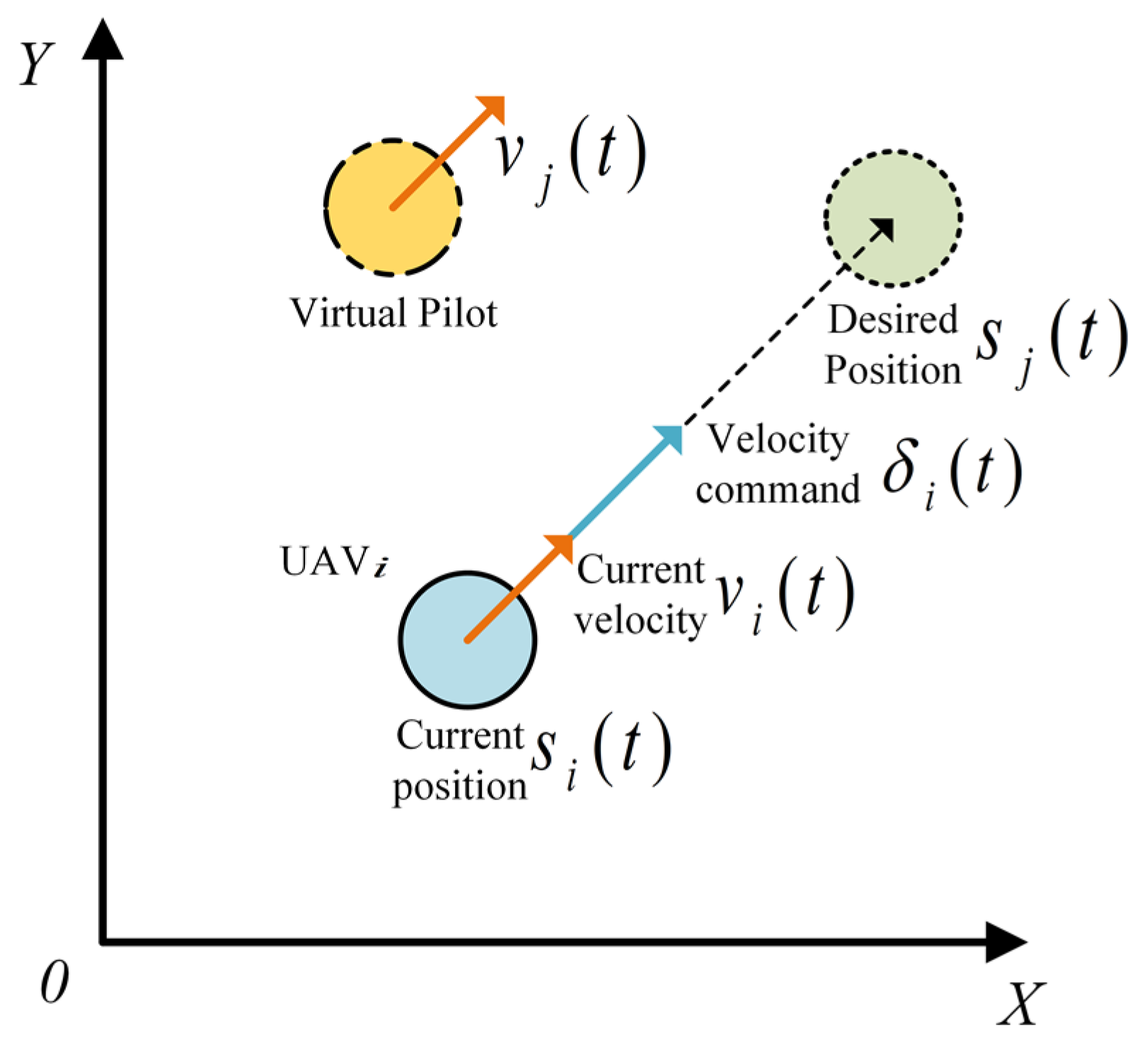
3.1. Virtual Pilot Formation-Control Algorithm

The UAV formation constructed in this study includes five drones, which is a relatively small number. The mathematical model of the leader–follower mode is easy to construct and has a simple structure. Therefore, the virtual pilot mode is considered for organizing the formation of UAVs. In this mode, all physical drones in the formation act as followers, while a virtual leading UAV is created through the control system and positioned at the center of formation. This virtual lead UAV is responsible for organizing the formation shape, navigation, obstacle avoidance, and target tracking. The UAVs are responsible for tracking the flight state and trajectory of the virtual lead UAV and maintaining their relative positions within the formation.

The objective of the UAV formation is for all UAVs to reach the desired position and desired velocity of the formation flight, as depicted in Equation (24).

$$\left\{\begin{array}{l}\underset{\mathrm{t}\to \infty }{\lim }(v_i\left(\mathrm{t}\right)-v_j\left(\mathrm{t}\right))=\overrightarrow{0} \\ \underset{\mathrm{t}\to \infty }{\lim }(s_i\left(\mathrm{t}\right)-s_j\left(\mathrm{t}\right))=\overrightarrow{0} \end{array}\right. ,$$

(24)

where $v_i\left(t\right)$ and $s_i\left(t\right)$ denote the current velocity vector and position vector of ${UAV}_i$ respectively, and $v_j\left(t\right)$ and $s_j\left(t\right)$ denote the desired velocity vector and position vector of ${UAV}_j$ respectively; $v_j\left(t\right)$ is also the current velocity vector of the virtual navigator. During the formation flight, the virtual navigator continuously sends its desired position to each UAV. Each UAV then acquires its own positional status and continuously adjusts itself to follow the desired position. The schematic diagram is shown in Figure 7.

The UAV control adopts the velocity command mode, i.e., the UAV can follow the input desired velocity and automatically adjust its own attitude using a proportional control strategy. The tracking of the virtual navigator’s position by the UAV is also introduced, as shown in Equation (25).

$${\delta }_i\left(\mathrm{t}\right)=v_j\left(\mathrm{t}\right)+\kappa \left(s_j\right(\mathrm{t})-s_i(\mathrm{t}\left)\right),$$

(25)

where ${\delta }_i\left(\mathrm{t}\right)$ represents the speed-control command sent to the ${UAV}_i$, $\kappa$ is a coefficient. In this way, the velocity of ${UAV}_i$ is not only affected by the difference between its desired position and its current position, but also by the current position of the virtual navigator. This allows the UAV to track its position while also tracking the velocity of the virtual navigator.

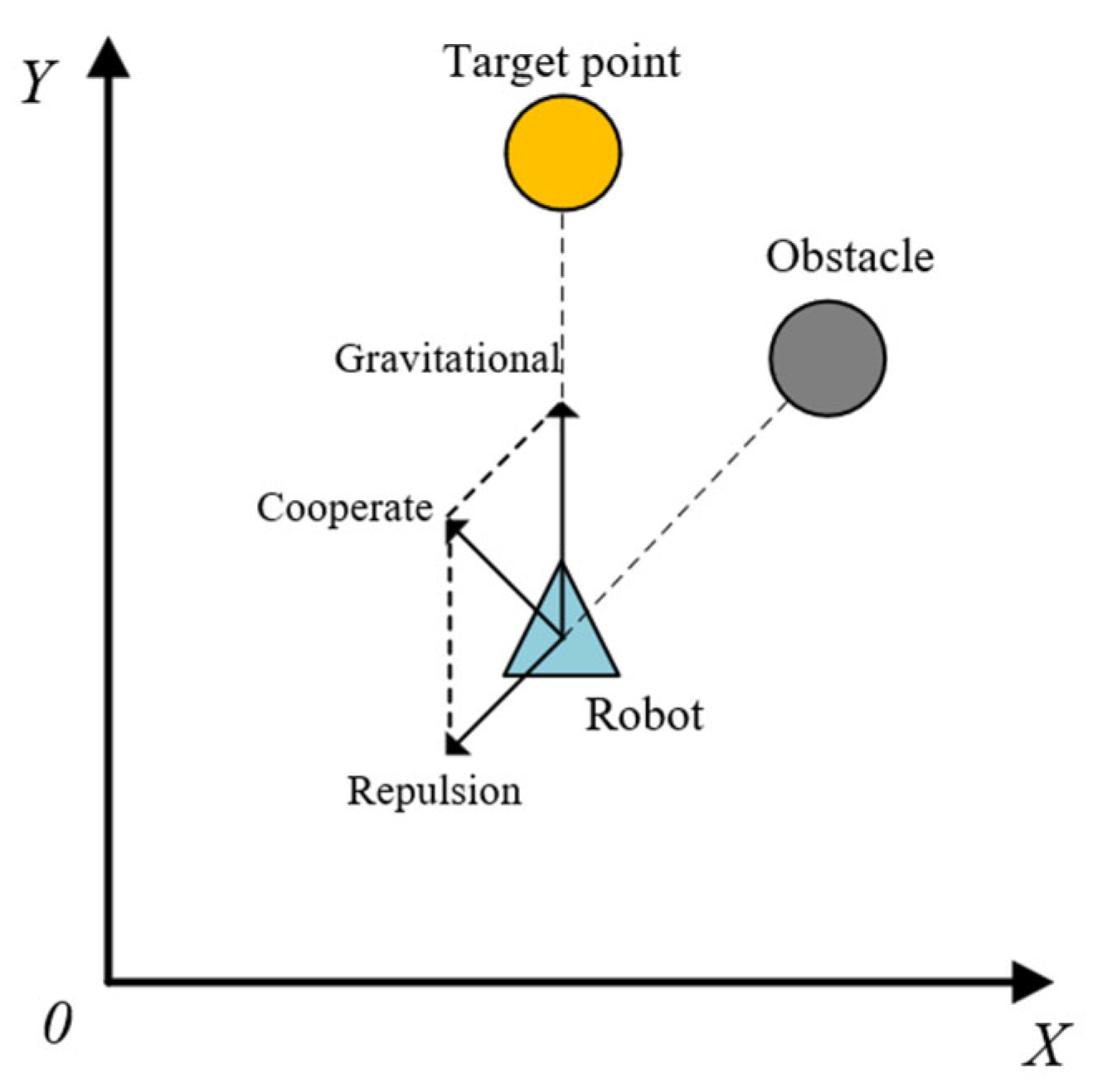
3.2. Global Artificial Potential Field Method

In this paper, a formation-control algorithm based on a virtual navigator is used to achieve multi-UAV formation organization and mission execution. During the formation flight, each UAV obtains its own position information and desired position information through local communication. It then adjusts its speed in real time to achieve the formation and control of multiple UAVs. In the given algorithm, the UAVs do not acquire or respond to the position information of other UAVs. Additionally, the UAVs are unable to perform evasive maneuvers to avoid obstacles in the environment. If no corresponding measures are taken, the UAVs may collide with obstacles and other UAVs during flight and formation switching.

This paper utilizes the artificial potential field method to address them. As mentioned earlier, the artificial potential field method can be utilized for path planning to avoid obstacles and impassable regions. It is also a widely adopted and effective approach for resolving collision issues. Therefore, the plan is to implement a multi-UAV collision-avoidance strategy based on the artificial potential field method.

Obstacles in the map are set to be saved as a priori information in a raster map, and UAV formations can read the location of the obstacles from the map between them during flight. The UAV calculates its own positional relationship with the obstacle in real time. When the distance from the obstacle is less than the obstacle repulsive field threshold, $p_{01}$, the UAV experiences an obstacle repulsive force. The repulsive force increases as the distance from the obstacle decreases. The obstacle potential field function is shown in Equation (26).

$$U_{iq}=\left\{\begin{array}{ll}{\displaystyle \frac{1}{2}}{\mu }_1({\displaystyle \frac{1}{p_{iq}}}-{\displaystyle \frac{1}{p_{01}}}{)}^2& , p_{iq}\le p_{01}\\ 0& , p_{iq}>p_{01}\end{array}\right. ,$$

(26)

where ${\mu }_1$ is a constant, $p_{iq}$ represents the distance between ${UAV}_i$ and obstacle $\mathrm{q}$, and ${\mathrm{p}}_{01}$ is a constant distance indicating the upper limit at which the obstacle generates a repulsive force. When $p_{iq}>p_{01}$, ${UAV}_i$ is not affected by the repulsive force from obstacle $q$. Therefore, the repulsive force of ${UAV}_i$ caused by obstacle $q$ is the negative derivative of ${\mathrm{U}}_{\mathrm{i}\mathrm{q}}$, which is ${\mathrm{F}}_{\mathrm{i}\mathrm{q}}$, as shown in Equation (27), where ${\mathrm{X}}_{\mathrm{i}}$ represents the current position vector of ${UAV}_i$.

$${\mathrm{F}}_{\mathrm{iq}}=-{\mathrm{grad}(\mathrm{U}}_{\mathrm{iq}})=\left\{\begin{array}{ll}{\mu }_1({\displaystyle \frac{1}{p_{iq}}}-{\displaystyle \frac{1}{p_{01}}}){\displaystyle \frac{1}{{p_{iq}}^2}}{\displaystyle \frac{\partial p_{iq}}{\partial {\mathrm{X}}_{\mathrm{i}}}}& , p_{iq}\le p_{01}\\ 0& , p_{iq}>p_{01}\end{array}\right. ,$$

(27)

All UAVs use broadcasting to transmit their own state information at a specific frequency. Additionally, all UAVs are capable of receiving the state information released by other UAVs. Therefore, with little network latency (millisecond latency), it can be assumed that each UAV in the UAV formation has access to the real-time positions of the other UAVs. When the distance between two UAVs is less than the threshold for the UAV repulsive field, both UAVs will experience a repulsive force on each other. The closer the distance, the stronger the repulsive force. Let UAV be subjected to the repulsive force field generated by other UAVs besides itself, and let the repulsive force field of UAV be as shown in Equation (28).

$$U_{iw}=\left\{\begin{array}{ll}{\displaystyle \frac{1}{2}}{\mu }_2({\displaystyle \frac{1}{p_{iw}}}-{\displaystyle \frac{1}{p_{02}}}{)}^2& , p_{iw}\le p_{02}\\ 0& , p_{iw}>p_{02}\end{array}\right. ,$$

(28)

where ${\mu }_2$ is a constant, $p_{iw}$ is the distance between ${UAV}_i$ and ${UAV}_w$, and $p_{02}$ is a distance constant indicating the upper limit of the distance at which the UAV generates a repulsive force. ${UAV}_i$ is not subjected to the repulsive force of ${UAV}_w$ when $p_{iw}>p_{02}$. Therefore, the repulsive force ${\mathrm{F}}_{\mathrm{i}\mathrm{w}}$ of ${UAV}_i$ by ${UAV}_w$ is the negative derivative of ${\mathrm{U}}_{\mathrm{i}\mathrm{w}}$, as shown in Equation (29).

$${\mathrm{F}}_{\mathrm{iw}}=-{\mathrm{grad}(\mathrm{U}}_{\mathrm{iw}})=\left\{\begin{array}{ll}{\mu }_2({\displaystyle \frac{1}{p_{iw}}}-{\displaystyle \frac{1}{p_{02}}}){\displaystyle \frac{1}{{p_{iw}}^2}}{\displaystyle \frac{\partial p_{iw}}{\partial {\mathrm{X}}_{\mathrm{i}}}}& , p_{iw}\le p_{02}\\ 0& , p_{iw}>p_{02}\end{array}\right. ,$$

(29)

Therefore, the total repulsive force field on the UAV is given by Equation (30).

$${\mathrm{U}}_{\mathrm{i}}=\sum {\mathrm{U}}_{\mathrm{i}\mathrm{q}}+\sum {\mathrm{U}}_{\mathrm{i}\mathrm{w}} ,$$

(30)

$${\mathrm{F}}_{\mathrm{i}}=\sum {\mathrm{F}}_{\mathrm{i}\mathrm{q}}+\sum {\mathrm{F}}_{\mathrm{i}\mathrm{w}} ,$$

(31)

The total repulsive force on UAV is in Equation (31).

4. Algorithm Validation

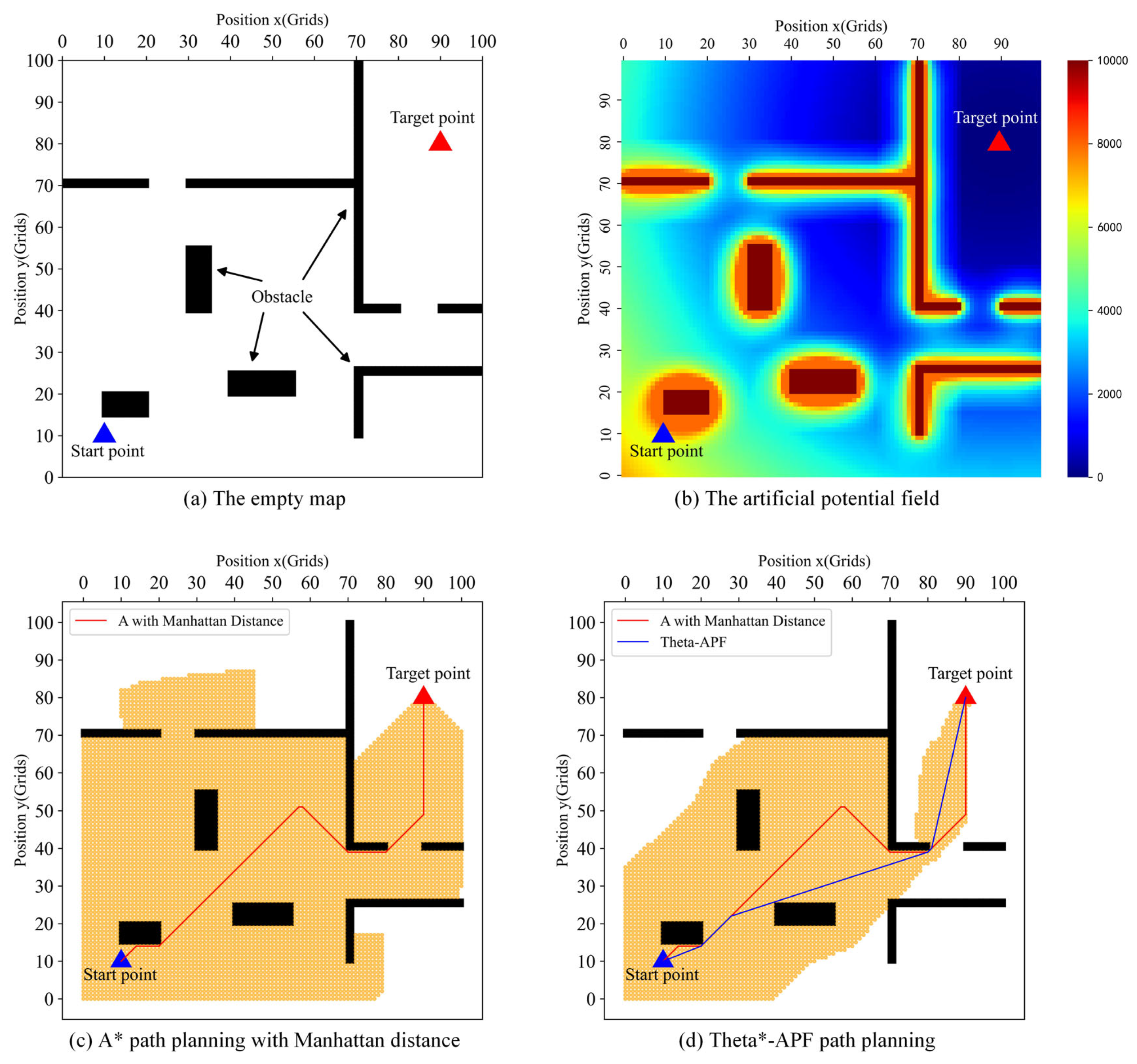
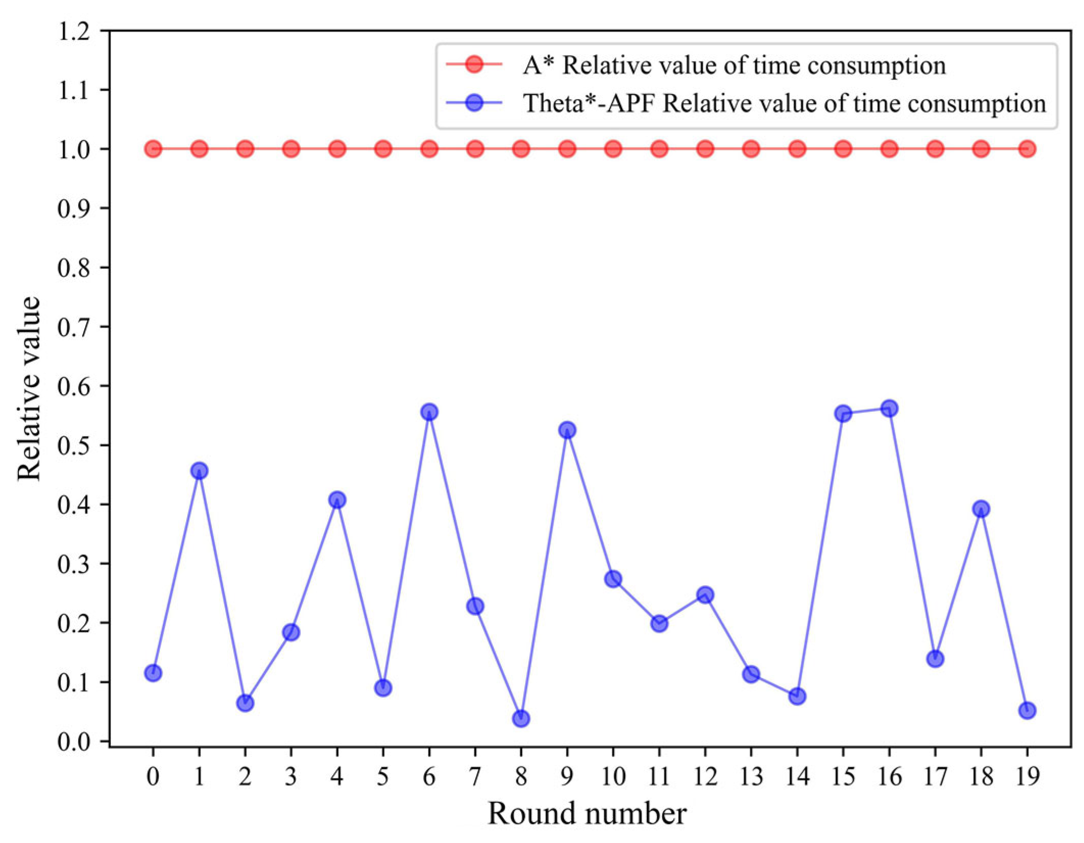
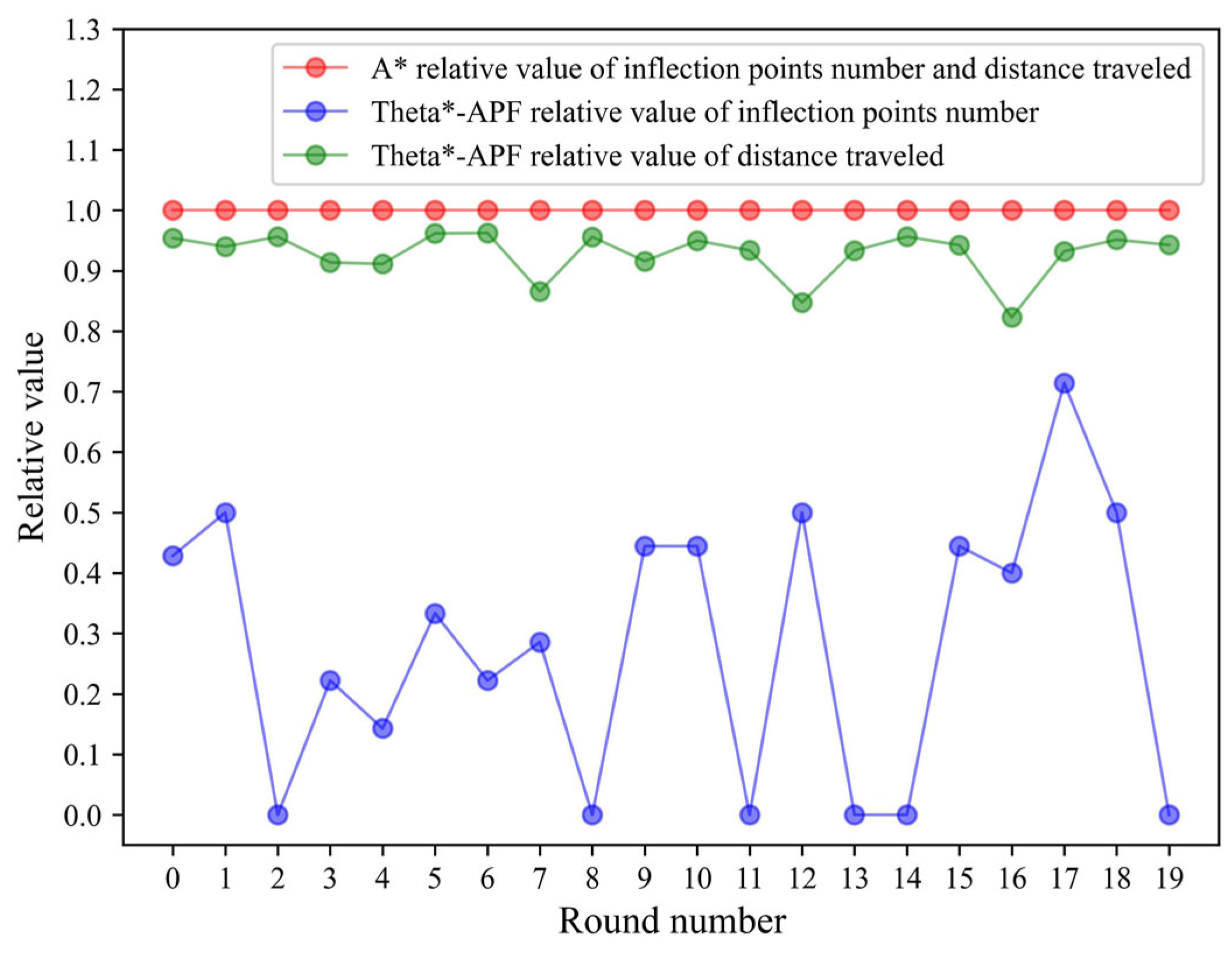
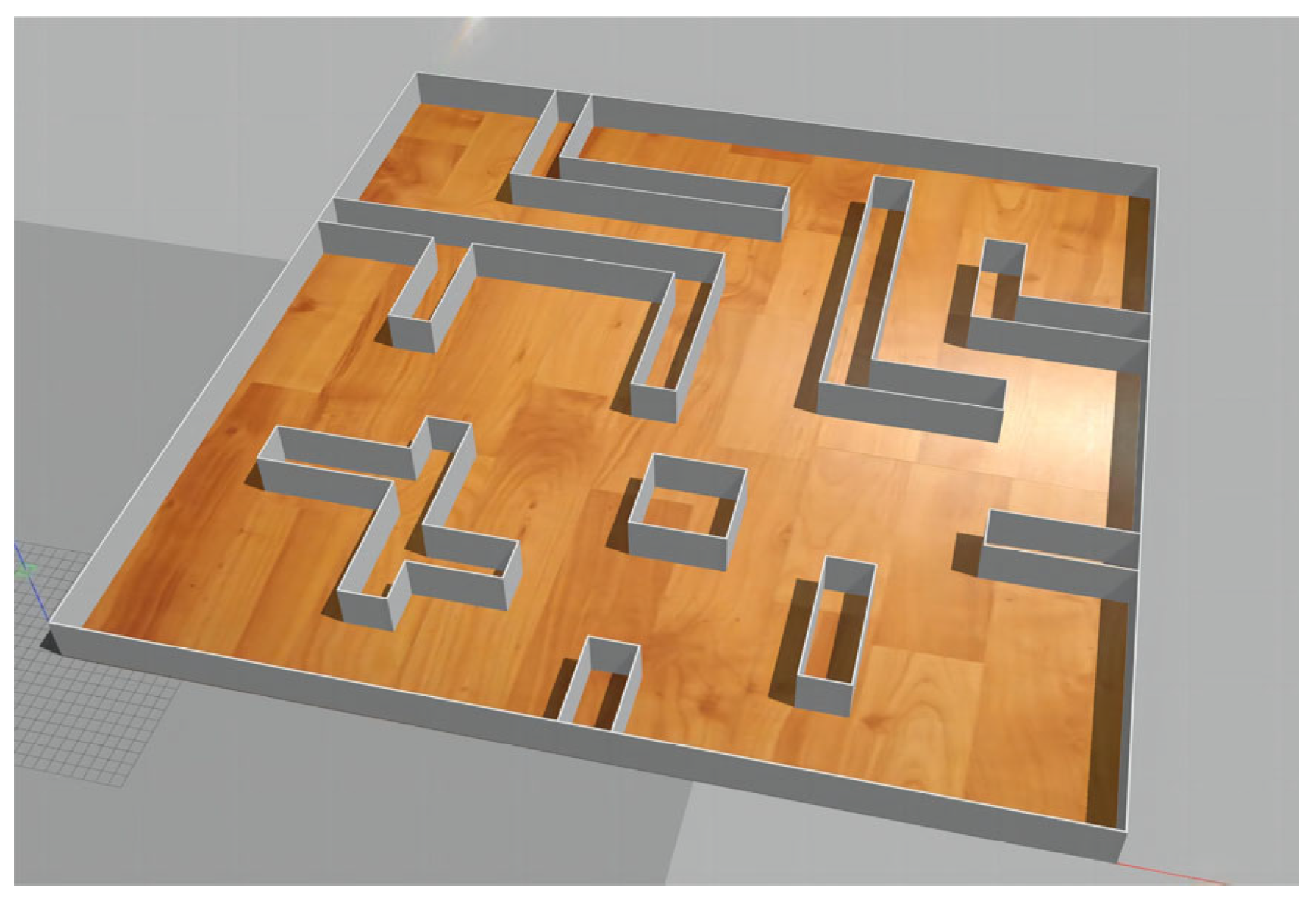
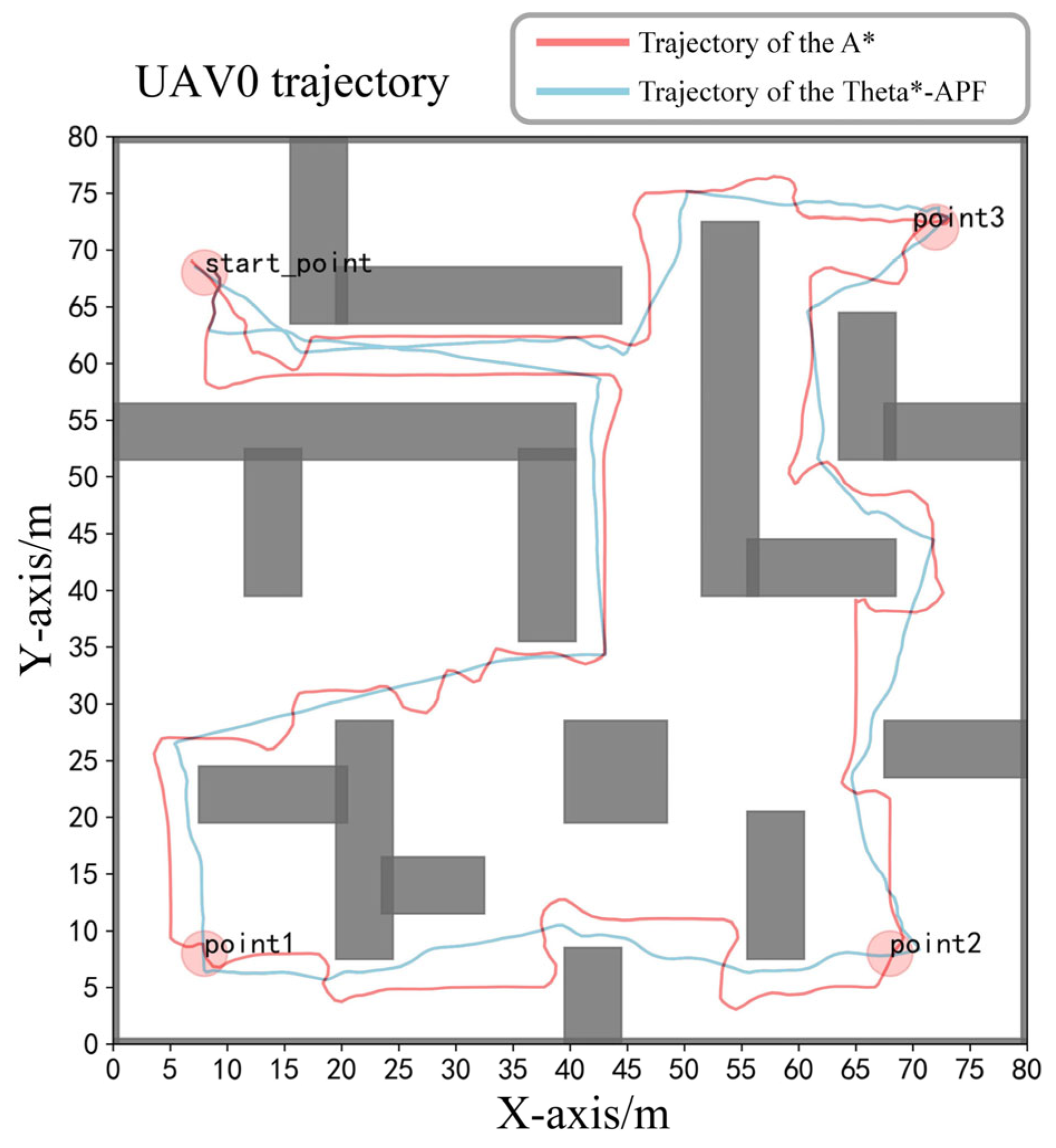
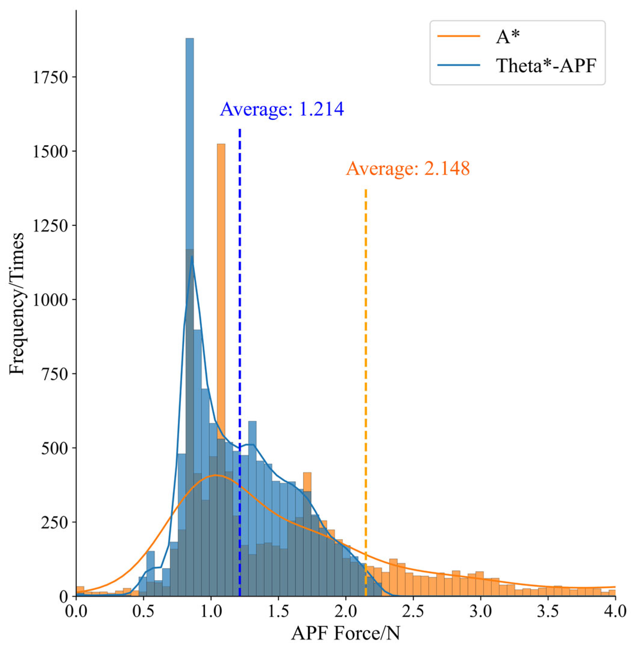
4.1. Simulation of Theta*–APF Algorithm Path Planning

In order to show the path-planning effect of the different algorithms more clearly and realize the comparison between different algorithms, we first carry out simulation experiments under the 2D raster map. In a 2D raster map with $100\times 100$ grid numbers, the starting point and the end point are selected, and the simulation experiments are performed for A* algorithm and Theta*–APF algorithm, respectively; the results are shown in Figure 8. Subfigure (a) is a blank map, the black part is the area of impassable obstacles, the blue triangles indicate the starting point, and the red triangles indicate the target point. Subfigure (b) shows the distribution of the artificial potential field strength throughout the map, where the obstacle region has the highest artificial potential field strength, the target point has the lowest artificial potential field strength, and the rest of the nodes have a corresponding increase in artificial potential field strength with the increase in distance from the target point. The strength distribution of the artificial potential field can be plotted more intuitively in a two-dimensional environment (the strength of the artificial potential field in a three-dimensional scenario is actually four-dimensional data, which is difficult to represent), which is the reason why a two-dimensional scenario is chosen for simulation in the first place. Subfigure (c) illustrates path planning using the traditional A* algorithm (using the Manhattan distance calculator as a heuristic function), where the yellow areas indicate the nodes that were processed during the path-search process, and the red line indicates the final planned path. Subfigure (d) shows the path planning results using the Theta*–APF algorithm for the same case, the planned paths are shown as blue lines in the figure, where the planning results of the A* algorithm are also plotted (red lines, consistent with subfigure (c)). Comparing subgraph (c) and subgraph (d) it can be clearly seen that the number of search nodes (yellow part) in the case of path planning using Theta*–APF algorithm is significantly smaller than that of path planning using A* algorithm.

The same results can be seen in

Table 1. Performance parameters of the A* algorithm and the Theta*–artificial potential field method algorithm.

Path-Planning Algorithm	Number of Search Nodes (Grids)	Path Length (Grids)	Inflection Number	Search Time
A* Manhattan distance calculation method	6679	137.095	6	21.666 s
Theta*–APF	4222	119.207	3	10.380 s

, which shows the specific data in the case of path planning using both algorithms, from which it can be seen that the Theta*–APF algorithm outperforms the traditional A* algorithm in all relevant metrics.

We conduct 20 rounds of round robin testing of the traditional A* neighborhood search algorithm and the Theta*–artificial potential field method path-planning algorithm. The A* algorithm chooses the Manhattan distance calculation method as the heuristic function. The A* algorithm and the Theta*–APF algorithm use the same start and end points in each round of testing. Figure 9 and Figure 10 show the test results, where the data of the A* algorithm are used as references (setting the data of the A* algorithm to 1), and the data are presented by the ratio of the data of the Theta*–artificial potential field method algorithm with respect to the data of the A* algorithm. Figure 9 shows the comparison of computational time consumption, in all rounds of testing, the Theta*–artificial potential field method algorithm computational time consumption is all less than the A* algorithm computational time consumption, distributed in the range of 10–60% of the A* algorithm; Figure 10 demonstrates the number of inflection points of the Theta*–artificial potential field method algorithm planning paths and the relative value of the length of paths compared with the A* algorithm, the blue line in the figure is the Theta*–artificial potential field method algorithm inflection point number and path length relative to the A* algorithm. The artificial potential field method algorithm inflection point length relative value, the green line is the Theta*–artificial potential field method algorithm journey length relative value; the Theta*–artificial potential field method algorithm journey length compared to the A* algorithm is reduced by about 10; the Theta*–artificial potential field method algorithm number of inflection points relative to the A* algorithm is reduced by 40–90%. Although the Theta*–APF algorithm is not stable enough in terms of optimization on all indicators (the variation of optimization effect is large), all indicators are much better than the A* algorithm.

We extend this 2D map in 3D and perform path planning with the same starting and ending points as Figure 8 (with the same coordinates mapped to the x–y plane), as shown in Figure 11. Moreover, when the map is expanded from a two-dimensional raster map to a three-dimensional voxel map, the increase in dimensionality will result in a geometric increase in the number of grids. This, in turn, will lead to an increase in the number of domains that need to be searched by each node. This increase is particularly problematic for the on-board computers of UAVs. As shown in Figure 12, when the map is expanded from 2D to 3D (assuming a height of 20 grids), the total number of grids will be expanded by 1900%, and if the traditional A* algorithm is used for path planning, its search time will be expanded from 21.666 s to 863.096 s, which is an increase of 3884%, whereas the path planning using the Theta*–APF algorithm for the same case will be expanded only from 10.380 s to 30.456 s, an increase of only 193.4%. The increase in computational time consumed by the Theta*–APF algorithm is significantly smaller than that using the traditional A* algorithm, which is due to the fact that the Theta*–APF algorithm employs the heuristic function of the artificial potential field method; its search will be more purposeful, and therefore exhibits higher efficiency in path planning in a three-dimensional environment.

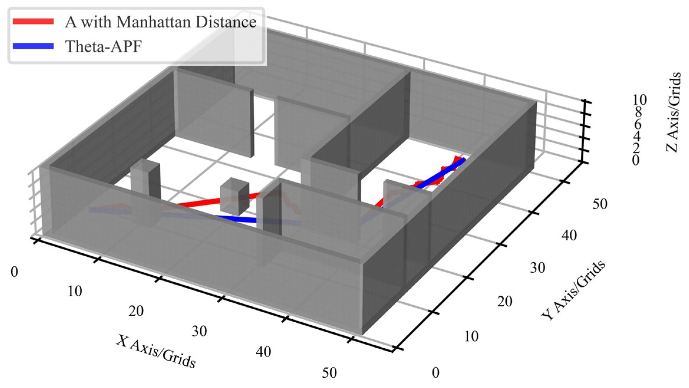
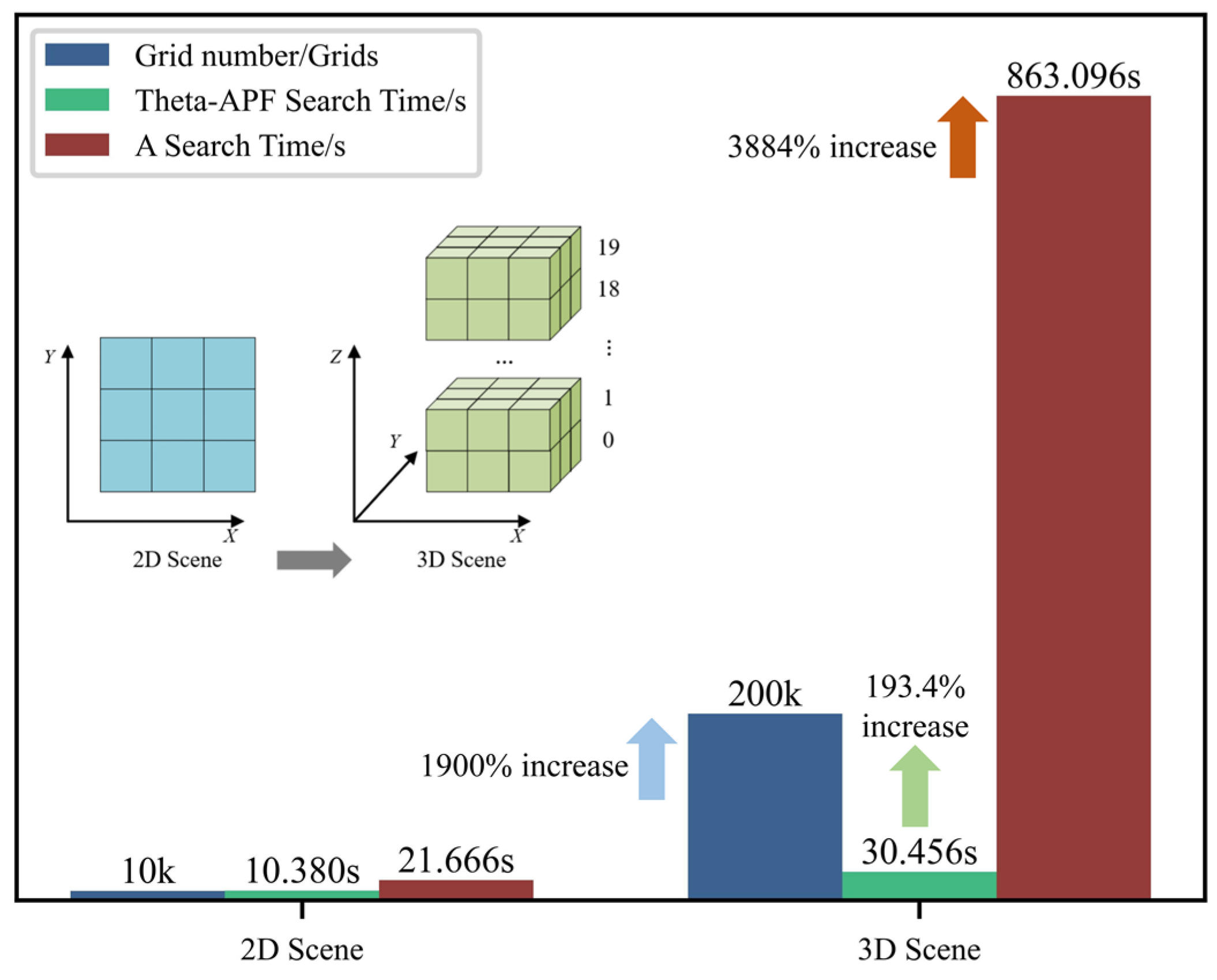
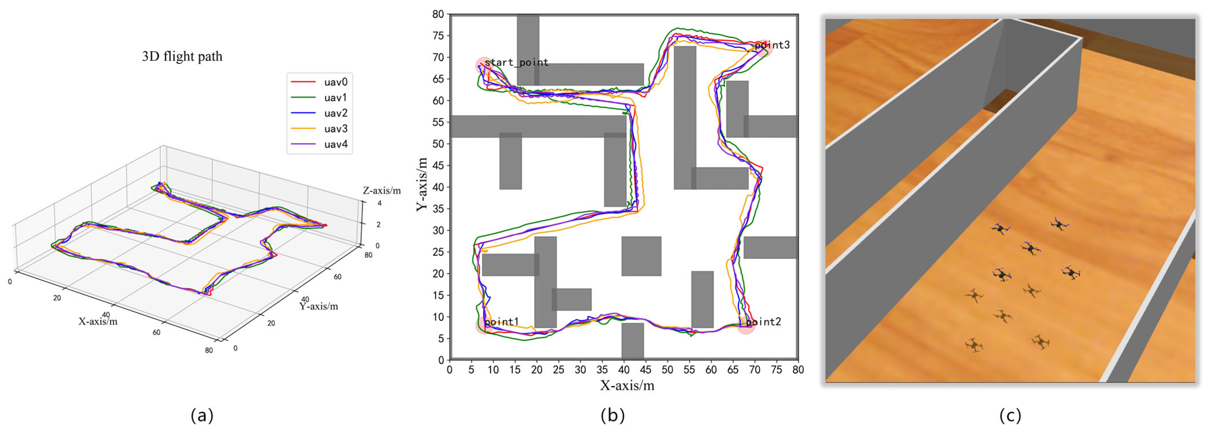
4.2. Simulation of UAV Formation Flight in 3D Environment

The simulation scenario used has dimensions of 80 m × 80 m × 4 m, and the obstacle setting is complex. The scenario simulates a large 3D indoor scene in which a formation of UAVs can fly in formation, with obstacles (gray part) set up to simulate items placed in an actual indoor environment. The simulation scenario is shown in Figure 13.

The formation of UAVs in the 3D simulation is achieved through the successive planning of multiple path points. This planning ultimately results in the formation of a loop, and the flight trajectory of the UAV is output and plotted in real time. This process is used to evaluate the efficiency and reliability of the Theta*–APF method for the 3D path-planning algorithm. Although our tests were conducted in a 3D simulation environment, most of the plots below are top views due to the difficulty in accurately comparing the strengths and weaknesses between multiple paths in 3D plots.

Figure 14 shows the flight trajectory of UAV0 (one of the aircrafts in the formation) under different path-planning algorithms. The red path is the flight trajectory under the A* algorithm and the blue path is the flight trajectory under the Theta*–APF algorithm.

As can be seen from the above trajectory diagrams, both algorithms are able to avoid obstacles and fly safely to the predefined target point when performing path planning. However, when the A* algorithm performs path planning, due to the limitation of the forward direction, the UAV’s trajectory is more like a zigzag in the vicinity of obstacles, turns, and diagonal movements, and does not find the shortest path; on the contrary, when the Theta*–APF algorithm performs path planning, the overall trajectory is smoother, and a shorter path is found. As shown in

Table 2. UAV0 flight distance for different path-planning algorithms.

Path-Planning Algorithm	Path Length (m)
A* algorithm	370.711
Theta*–APF	325.321

, the distance traveled by the UAV0 flight trajectory varies with different algorithms, and the distance traveled by the Theta*–APF algorithm decreases by about 12% compared to the A* algorithm when planning the path.

During flight, UAVs are continuously affected by artificial potential field forces generated by the surrounding obstacles, which leads to spontaneous obstacle avoidance. The closer the UAV is to the obstacle, the greater the repulsive force effect by the obstacle is; therefore, we use the size of the artificial potential field repulsive force of the obstacle to which no UAV formation is subjected to measure the distance and proximity of the UAV to the surrounding obstacles during the UAV formation flight process, and then compare the ability of the Theta*–APF algorithm and the A* algorithm to guide the safe flight of the UAV formation under the environment of complex obstacles. As shown in Figure 15, we plot the histograms of the magnitude of the artificial potential field force on the UAV formation during UAV formation flight under the A* algorithm and the Theta*–APF algorithm, respectively. The x-axis data represent the magnitude of the artificial potential field force, and the y-axis represents the frequency of occurrence of this value throughout the flight (cumulative number of times). It is shown that, when using the Theta*–APF algorithm, the UAV is subjected to less force from the obstacle artificial potential field for most of the flight compared to that using the A* algorithm (the peaks of the data frequencies are closer to the zero point); the peaks of the force using the A* algorithm are much larger than those using the Theta*–APF algorithm (extending over a wider range of the x-axis). We have also plotted the average value of the artificial potential field force for the different algorithms, where the force decreases by about 42.039% (from 2.148 to 1.245) using the Theta*–APF algorithm compared to the traditional A* algorithm. This indicates that using the Theta*–APF algorithm to guide the UAV formation flight will have higher safety than using the A* algorithm.

Based on the above simulations and comparative experiments, we have basically verified that the Theta*–APF algorithm has significant advantages over the traditional A* algorithm in terms of path planning time, distance traveled, path smoothing, and the safety of guiding UAV formations to fly in an obstacle environment. Figure 16a,b illustrate the 3D and 2D images of the flight trajectory of each UAV during formation flight, respectively. Figure 16c shows the formation (diamond-shaped formation) maintained by the UAV formation at any moment of the flight, which always flies in such a formation to achieve obstacle avoidance as well as to avoid collisions between UAVs through localized squeezing and deformation of the formation. The UAV formation successfully maintains formation safe flight in complex obstacle environments, which further validates the effectiveness and reliability of our proposed algorithm.

5. Conclusions and Future Works

In this paper, a new point-to-point path-planning algorithm, the Theta*–APF algorithm, is proposed and applied to UAV formation flying in obstacle environments. The Theta*–APF algorithm has been improved compared to the A* algorithm mainly in the heuristic function and forward direction, which is based on the principle of the artificial potential field algorithm, which is used as a heuristic function to improve the A* algorithm, and introduces the widely used inverse reasoning strategy to optimize the A* algorithm into the Theta* algorithm, resulting in the Theta*–APF algorithm. The simulation and comparison experiments basically verified that the Theta*–APF algorithm has significant advantages over the A* algorithm in terms of search time, path superiority and inferiority, and safety of UAV formation flight.

Due to various limitations, this study did not utilize physical drones for experiments. Therefore, further research and validation are needed to assess the reliability and robustness of the proposed algorithm in real-world settings. In future work, we also plan to deploy the algorithm into specific UAVs for formation flight experiments. The Theta*–APF algorithm proposed in this paper can be easily adapted to UAV formation path planning situations in 3D environments. In addition, we will conduct further research on the organization of UAV formations and apply the algorithm to larger scale formation flights and more complex environments.

References

1. Zhang, J.; Yan, J.; Zhang, P. Multi-UAV Formation Control Based on a Novel Back-Stepping Approach. IEEE Trans. Veh. Technol. 2020, 69, 2437–2448. [Google Scholar] [CrossRef]
2. Shao, S.; Peng, Y.; He, C.; Du, Y. Efficient Path Planning for UAV Formation via Comprehensively Improved Particle Swarm Optimization. ISA Trans. 2020, 97, 415–430. [Google Scholar] [CrossRef] [PubMed]
3. Warren, C.W. Global Path Planning Using Artificial Potential Fields. In Proceedings of the 1989 IEEE International Conference on Robotics and Automation, Scottsdale, AZ, USA, 14–19 May 1989; IEEE Computer Society: Washington, DC, USA, 1989; pp. 316–317. [Google Scholar]
4. Chang, L.; Shan, L.; Jiang, C.; Dai, Y. Reinforcement Based Mobile Robot Path Planning with Improved Dynamic Window Approach in Unknown Environment. Auton. Robot. 2021, 45, 51–76. [Google Scholar] [CrossRef]
5. Zhu, Z.; Xie, J.; Wang, Z. Global Dynamic Path Planning Based on Fusion of A* Algorithm and Dynamic Window Approach. In Proceedings of the 2019 Chinese Automation Congress (CAC), Hangzhou, China, 22–24 November 2019; IEEE: Piscataway, NJ, USA, 2019; pp. 5572–5576. [Google Scholar]
6. Jin, Q.; Tang, C.; Cai, W. Research on Dynamic Path Planning Based on the Fusion Algorithm of Improved Ant Colony Optimization and Rolling Window Method. IEEE Access 2021, 10, 28322–28332. [Google Scholar] [CrossRef]
7. Kothari, M.; Postlethwaite, I. A Probabilistically Robust Path Planning Algorithm for UAVs Using Rapidly-Exploring Random Trees. J. Intell. Robot. Syst. 2013, 71, 231–253. [Google Scholar] [CrossRef]
8. Janoš, J.; Vonásek, V.; Pěnička, R. Multi-Goal Path Planning Using Multiple Random Trees. IEEE Robot. Autom. Lett. 2021, 6, 4201–4208. [Google Scholar] [CrossRef]
9. Wang, H.; Yu, Y.; Yuan, Q. Application of Dijkstra Algorithm in Robot Path-Planning. In Proceedings of the 2011 Second International Conference on Mechanic Automation and Control Engineering, Hohhot, China, 15–17 July 2011; IEEE: Piscataway, NJ, USA, 2011; pp. 1067–1069. [Google Scholar]
10. Mesquita, R.; Gaspar, P.D. A Path Planning Optimization Algorithm Based on Particle Swarm Optimization for UAVs for Bird Monitoring and Repelling–Simulation Results. In Proceedings of the 2020 International Conference on Decision Aid Sciences and Application (DASA), Sakheer, Bahrain, 8–9 November 2020; IEEE: Piscataway, NJ, USA, 2020; pp. 1144–1148. [Google Scholar]
11. Sharma, A.; Shoval, S.; Sharma, A.; Pandey, J.K. Path Planning for Multiple Targets Interception by the Swarm of UAVs Based on Swarm Intelligence Algorithms: A Review. IETE Tech. Rev. 2022, 39, 675–697. [Google Scholar] [CrossRef]
12. Pan, Z.; Zhang, C.; Xia, Y.; Xiong, H.; Shao, X. An Improved Artificial Potential Field Method for Path Planning and Formation Control of the Multi-UAV Systems. IEEE Trans. Circuits Syst. II Express Briefs 2021, 69, 1129–1133. [Google Scholar] [CrossRef]
13. Liu, H.; Chen, J.; Feng, J.; Zhao, H. An Improved RRT* UAV Formation Path Planning Algorithm Based on Goal Bias and Node Rejection Strategy. Unmanned Syst. 2023, 11, 317–326. [Google Scholar] [CrossRef]
14. Hoang, V.; Phung, M.D.; Dinh, T.H.; Ha, Q.P. Angle-Encoded Swarm Optimization for Uav Formation Path Planning. In Proceedings of the 2018 IEEE/RSJ International Conference on Intelligent Robots and Systems (IROS), Madrid, Spain, 1–5 October 2018; IEEE: Piscataway, NJ, USA, 2018; pp. 5239–5244. [Google Scholar]
15. Chen, H.; Chen, H.; Qiang, L. Multi-UAV 3D Formation Path Planning Based on Improved Artificial Potential Field. J. Syst. Simul. 2020, 32, 414–420. [Google Scholar]
16. Chen, Q.; Lu, Y.; Jia, G.; Li, Y.; Zhu, B.; Lin, J. Path Planning for UAVs Formation Reconfiguration Based on Dubins Trajectory. J. Cent. South Univ. 2018, 25, 2664–2676. [Google Scholar] [CrossRef]
17. Wu, Z.; Li, J.; Zuo, J.; Li, S. Path Planning of UAVs Based on Collision Probability and Kalman Filter. IEEE Access 2018, 6, 34237–34245. [Google Scholar] [CrossRef]
18. Luis, C.E.; Schoellig, A.P. Trajectory Generation for Multiagent Point-to-Point Transitions via Distributed Model Predictive Control. IEEE Robot. Autom. Lett. 2019, 4, 375–382. [Google Scholar] [CrossRef]
19. Palossi, D.; Furci, M.; Naldi, R.; Marongiu, A.; Marconi, L.; Benini, L. An Energy-Efficient Parallel Algorithm for Real-Time near-Optimal Uav Path Planning. In Proceedings of the ACM International Conference on Computing Frontiers, Como, Italy, 16–19 May 2016; pp. 392–397. [Google Scholar]
20. Yao, J.; Lin, C.; Xie, X.; Wang, A.J.; Hung, C.-C. Path Planning for Virtual Human Motion Using Improved A* Star Algorithm. In Proceedings of the 2010 Seventh International Conference on Information Technology: New Generations, Las Vegas, NV, USA, 12–14 April 2010; IEEE: Piscataway, NJ, USA, 2010; pp. 1154–1158. [Google Scholar]
21. Zhang, J.; Li, J.; Yang, H.; Feng, X.; Sun, G. Complex Environment Path Planning for Unmanned Aerial Vehicles. Sensors 2021, 21, 5250. [Google Scholar] [CrossRef] [PubMed]
22. Zhou, Z.; Wang, J.; Zhu, Z.; Yang, D.; Wu, J. Tangent Navigated Robot Path Planning Strategy Using Particle Swarm Optimized Artificial Potential Field. Optik 2018, 158, 639–651. [Google Scholar] [CrossRef]
23. Mai, X.; Li, D.; Ouyang, J.; Luo, Y. An Improved Dynamic Window Approach for Local Trajectory Planning in the Environment with Dense Objects. In Journal of Physics: Conference Series; IOP Publishing: Bristol, UK, 2021; Volume 1884, p. 012003. [Google Scholar] [CrossRef]
24. Fan, D.; Shi, P. Improvement of Dijkstra’s Algorithm and Its Application in Route Planning. In Proceedings of the 2010 Seventh International Conference on Fuzzy Systems and Knowledge Discovery, Yantai, China, 10–12 August 2010; IEEE: Piscataway, NJ, USA, 2010; Volume 4, pp. 1901–1904. [Google Scholar]
25. Chen, J.; Li, M.; Yuan, Z.; Gu, Q. An Improved A* Algorithm for UAV Path Planning Problems. In Proceedings of the 2020 IEEE 4th Information Technology, Networking, Electronic and Automation Control Conference (ITNEC), Chongqing, China, 12–14 June 2020; IEEE: Piscataway, NJ, USA, 2020; Volume 1, pp. 958–962. [Google Scholar]
26. Sánchez-Ibáñez, J.R.; Pérez-del-Pulgar, C.J.; García-Cerezo, A. Path Planning for Autonomous Mobile Robots: A Review. Sensors 2021, 21, 7898. [Google Scholar] [CrossRef] [PubMed]
27. Desai, J.P.; Ostrowski, J.; Kumar, V. Controlling Formations of Multiple Mobile Robots. In Proceedings of the 1998 IEEE International Conference on Robotics and Automation (Cat. No. 98CH36146), Leuven, Belgium, 20–20 May 1998; IEEE: Piscataway, NJ, USA, 1998; Volume 4, pp. 2864–2869. [Google Scholar]
28. Weitzenfeld, A.; Vallesa, A.; Flores, H. A Biologically-Inspired Wolf Pack Multiple Robot Hunting Model. In Proceedings of the 2006 IEEE 3rd Latin American Robotics Symposium, Santiago, Chile, 26–27 October 2006; IEEE: Piscataway, NJ, USA, 2006; pp. 120–127. [Google Scholar]
29. Lewis, M.A.; Tan, K.-H. High Precision Formation Control of Mobile Robots Using Virtual Structures. Auton. Robot. 1997, 4, 387–403. [Google Scholar] [CrossRef]
30. Persson, S.M.; Sharf, I. Sampling-Based A* Algorithm for Robot Path-Planning. Int. J. Robot. Res. 2014, 33, 1683–1708. [Google Scholar] [CrossRef]
31. Souissi, O.; Benatitallah, R.; Duvivier, D.; Artiba, A.; Belanger, N.; Feyzeau, P. Path Planning: A 2013 Survey. In Proceedings of the 2013 International Conference on Industrial Engineering and Systems Management (IESM), Rabat, Morocco, 28–30 October 2013; IEEE: Piscataway, NJ, USA, 2013; pp. 1–8. [Google Scholar]
32. Daniel, K.; Nash, A.; Koenig, S.; Felner, A. Theta*: Any-Angle Path Planning on Grids. J. Artif. Intell. Res. 2010, 39, 533–579. [Google Scholar] [CrossRef]
Figure 1. Traditional A* algorithm with 8-neighborhood search.
Drones 08 00125 g001
Figure 2. Optimization of the Theta* algorithm for the A* algorithm.
Drones 08 00125 g002
Figure 3. Schematic diagram of an artificial potential field, the change in color from blue to red represents an increase in the strength of the artificial potential field.
Drones 08 00125 g003
Figure 4. Schematic representation of the forces on the robot under an artificial potential field.
Drones 08 00125 g004
Figure 5. Schematic of mobile costing.
Drones 08 00125 g005
Figure 6. Schematic diagram illustrating the action of the heuristic function h (n) using the artificial potential field.
Drones 08 00125 g006
Figure 7. Schematic diagram of the drone-control method.
Drones 08 00125 g007
Figure 8. Simulation of Theta*–APF algorithm path planning.
Drones 08 00125 g008
Figure 9. Comparison of computational time consumption between A* and Theta*–artificial potential field method algorithm.
Drones 08 00125 g009
Figure 10. Comparison of the number of inflection points and distance traveled between the A* and the Theta*–APF algorithm.
Drones 08 00125 g010
Figure 11. Path planning in a 3D environment.
Drones 08 00125 g011
Figure 12. Changes in the number of search grids and search time from 2D to 3D maps.
Drones 08 00125 g012
Figure 13. Gazebo simulation scene.
Drones 08 00125 g013
Figure 14. UAV0 flight trajectory under A* algorithm and Theta*–APF algorithm.
Drones 08 00125 g014
Figure 15. Histogram of forces in the artificial potential field.
Drones 08 00125 g015
Figure 16. UAV formation flight trajectories in (a) 3D and (b) 2D environment and UAV formation schema (c).
Drones 08 00125 g016