Article

Comparative Analysis of the Impact of Additively Manufactured Polymer Tools on the Fiber Configuration of Injection Molded Long-Fiber-Reinforced Thermoplastics

1
Institute of Polymer Technology, University of Erlangen-Nuremberg, 91058 Erlangen, Germany
2
Department of Additive Manufacturing, BMW Group, 85764 Oberschleissheim, Germany
3
Department of Mechanical Engineering, Professorship of Laser-Based Additive Manufacturing, Technical University of Munich, 85748 Munich, Germany
4
Mechanical Engineering Department, Polymer Engineering Center, University of Wisconsin-Madison, Madison, WI 53706, USA
*
Author to whom correspondence should be addressed.
Contributed equally to this work.
J. Compos. Sci. 2020, 4(3), 136; https://0-doi-org.brum.beds.ac.uk/10.3390/jcs4030136
Submission received: 7 August 2020 / Revised: 7 September 2020 / Accepted: 11 September 2020 / Published: 15 September 2020
(This article belongs to the Special Issue Discontinuous Fiber Composites, Volume II)

Abstract

:
Additive tooling (AT) utilizes the advantages of rapid tooling development while minimizing geometrical limitations of conventional tool manufacturing such as complex design of cooling channels. This investigation presents a comparative experimental analysis of long-fiber-reinforced thermoplastic parts (LFTs), which are produced through additively manufactured injection molding polymer tools. After giving a review on the state of the art of AT and LFTs, additive manufacturing (AM) plastic tools are compared to conventionally manufactured steel and aluminum tools toward their qualification for spare part and small series production as well as functional validation. The assessment of the polymer tools focuses on three quality criteria concerning the LFT parts: geometrical accuracy, mechanical properties, and fiber configuration. The analysis of the fiber configuration includes fiber length, fiber concentration, and fiber orientation. The results show that polymer tools are fully capable of manufacturing LFTs with a cycle number within hundreds before showing critical signs of deterioration or tool failure. The produced LFTs moldings provide sufficient quality in geometrical accuracy, mechanical properties, and fiber configuration. Further, specific anomalies of the fiber configuration can be detected for all tool types, which include the occurrence of characteristic zones dependent on the nominal fiber content and melt flow distance. Conclusions toward the improvement of additively manufactured polymer tool life cycles are drawn based on the detected deteriorations and failure modes.

1. Introduction

1.1. Motivation

In the most recent decades, the ease of processability of long-fiber-reinforced thermoplastics (LFT) has enabled their use as advanced lightweight engineering materials, particularly within the automotive sector [1,2]. As a key technology, the injection molding process is expected to take a major role in terms of value and volume [3]. With an estimated market volume percentage of 65%, polypropylene (PP) is the material with the biggest market volume of LFTs in this field [4]. Material glass is predominantly used for reinforcement due to its low cost and superior mechanical properties [5].
Additive manufacturing (AM) is becoming increasingly important in industry in general and is becoming especially important in the automotive sector [6]. Although a lot of research and development is carried out, AM is still very limited in its available range of materials, which prevents its widespread entry into large-scale industry [7]. Due to its generative layer structure, most of the materials show lower molecular cohesion in one or more load directions [8]. Consequently, anisotropic material properties that deviate from those of the injection molded (IM) pedant must be expected [9]. This counts particularly for polymers; therefore, commodity construction materials such as PP, PU, PA, PC, blends, and other compounds can only be substituted to a very limited amount [10].
Additive tooling (AT) describes a process which combines the potential of AM with the material spectrum of a traditional manufacturing process, such as IM, by replacing the molding tool unit by an additive one and keeping the existing equipment of the traditional manufacturing technology alive. In this way, it is possible to produce moldings with series properties, to reduce the cost and time-consuming tool manufacturing process, and to increase the tooling complexity and the resulting part design freedom at the same time [11,12]. For this procedure, polymer molds are currently preferred due to their superior surface quality, lower production time, and lower costs in comparison to its metal pedant [13]. For AT, the most important production method is stereolithography (SL), which provides supreme surfaces with a high geometrical accuracy and the access to cross-linked and reinforced polymers. These composites are based on a high-temperature resistant polymer matrix which is enhanced with fillers such as aluminum or ceramics particles to improve the thermal conductivity, heat deflection point, and mechanical properties [14,15]. In general, plastic molds show a significant deviation from the conventional steel tools in points of heat capacity as well as in their temperature and thermal conductivity around a factor of 10 to 100 [16]. As the properties and behavior of plastic components are mainly defined by their thermal history, the cooling process of the polymer tools is crucial for the morphology and the crystallization of the moldings.
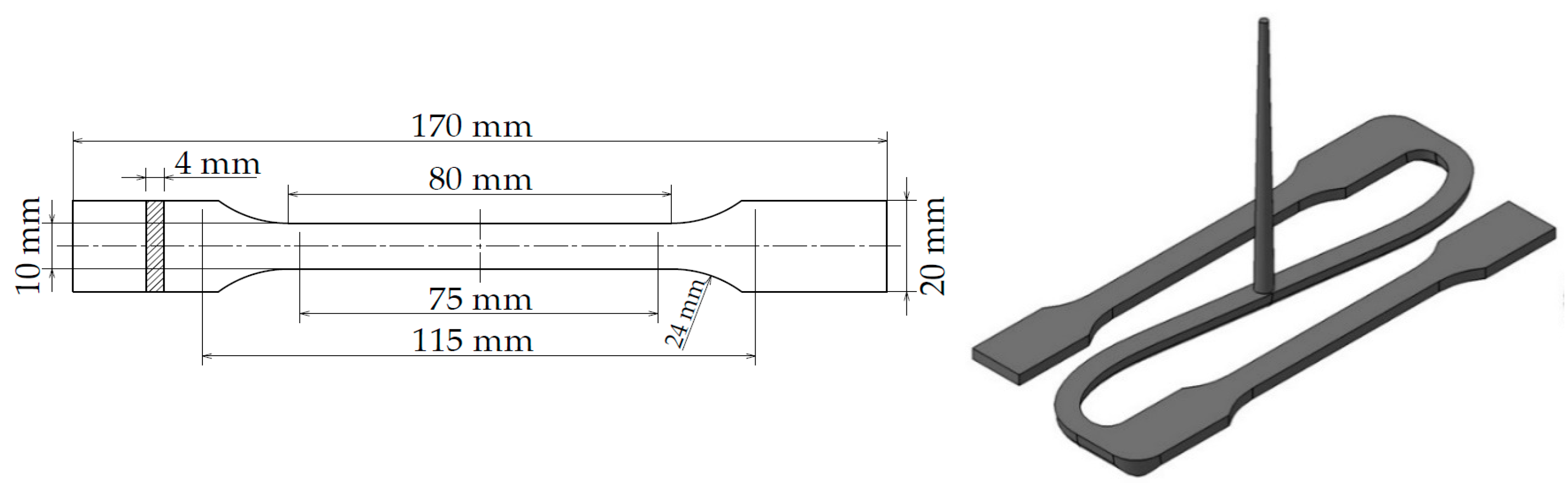
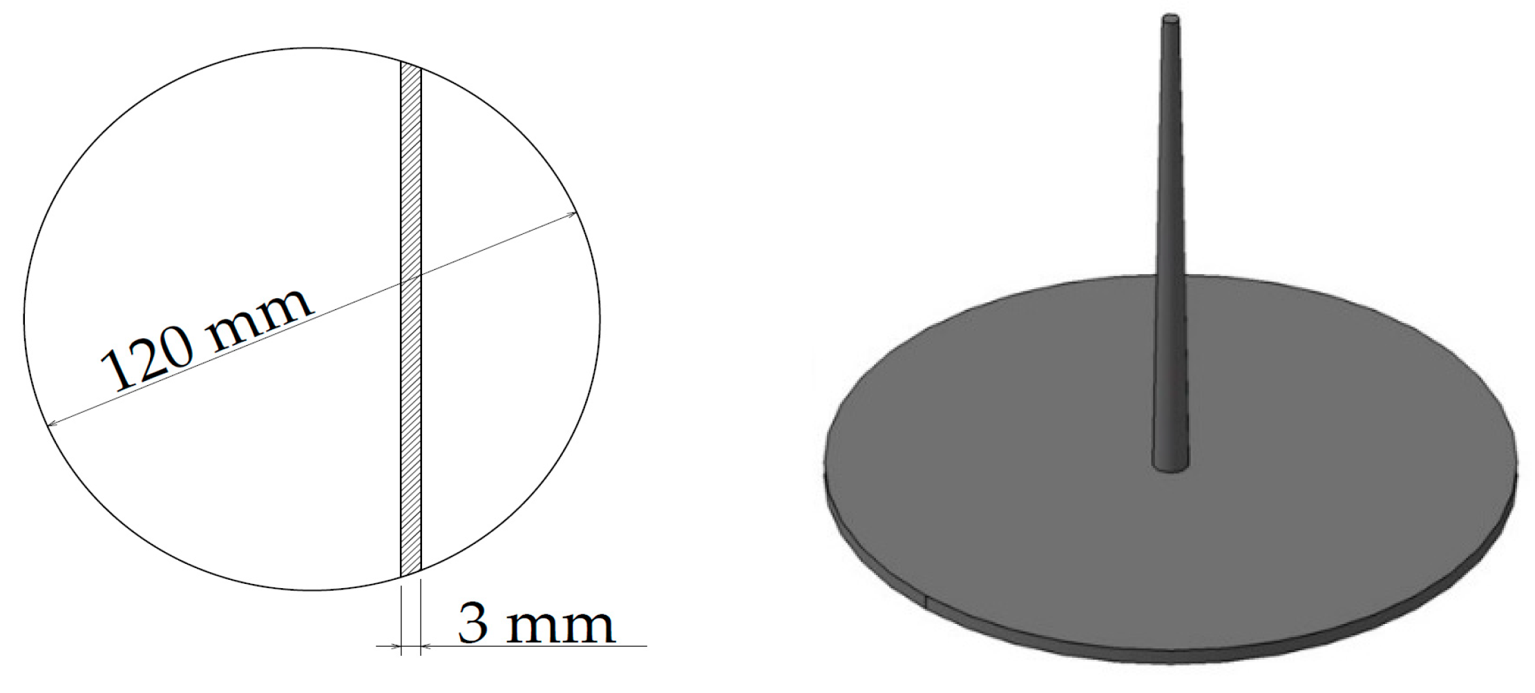
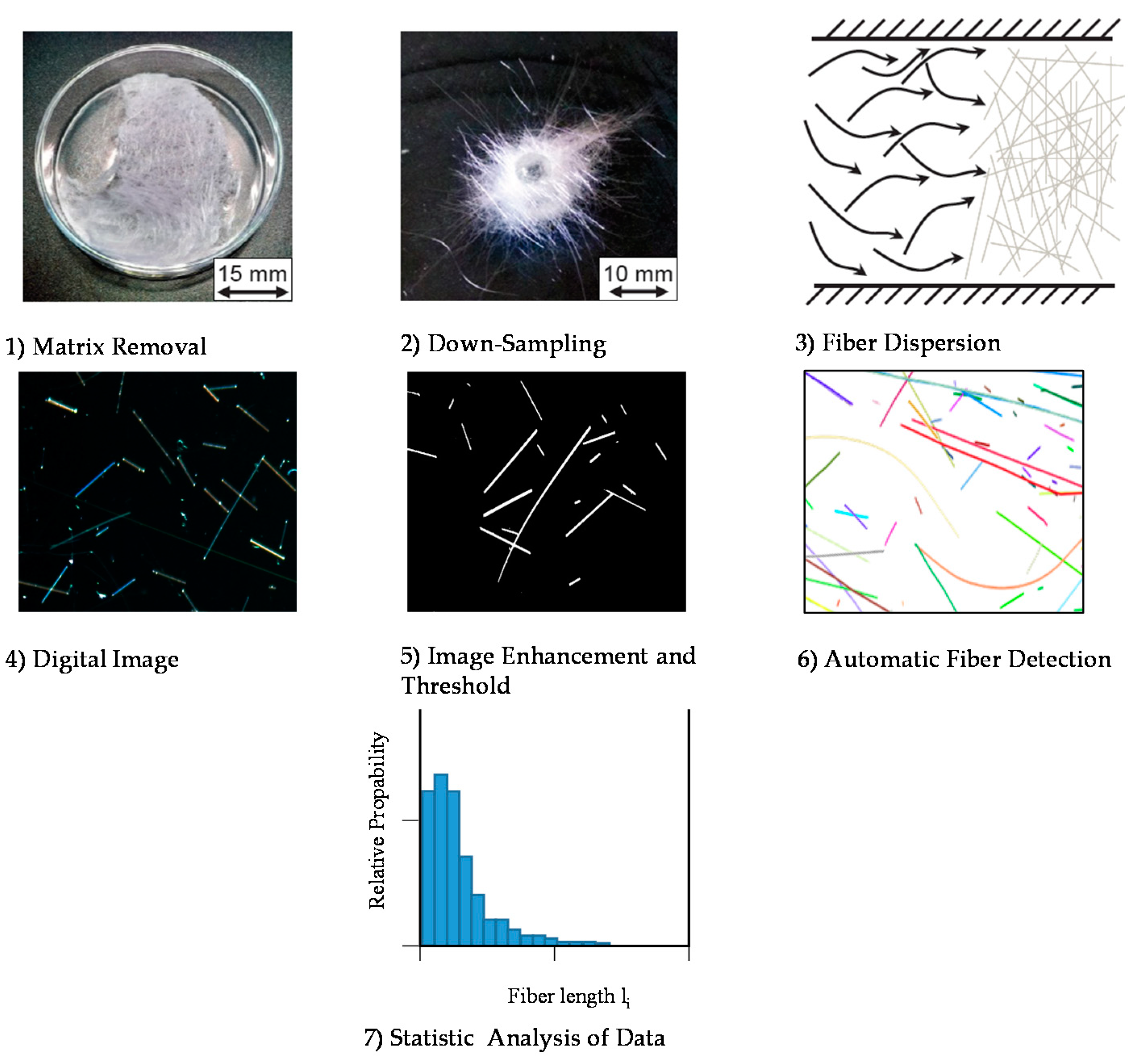
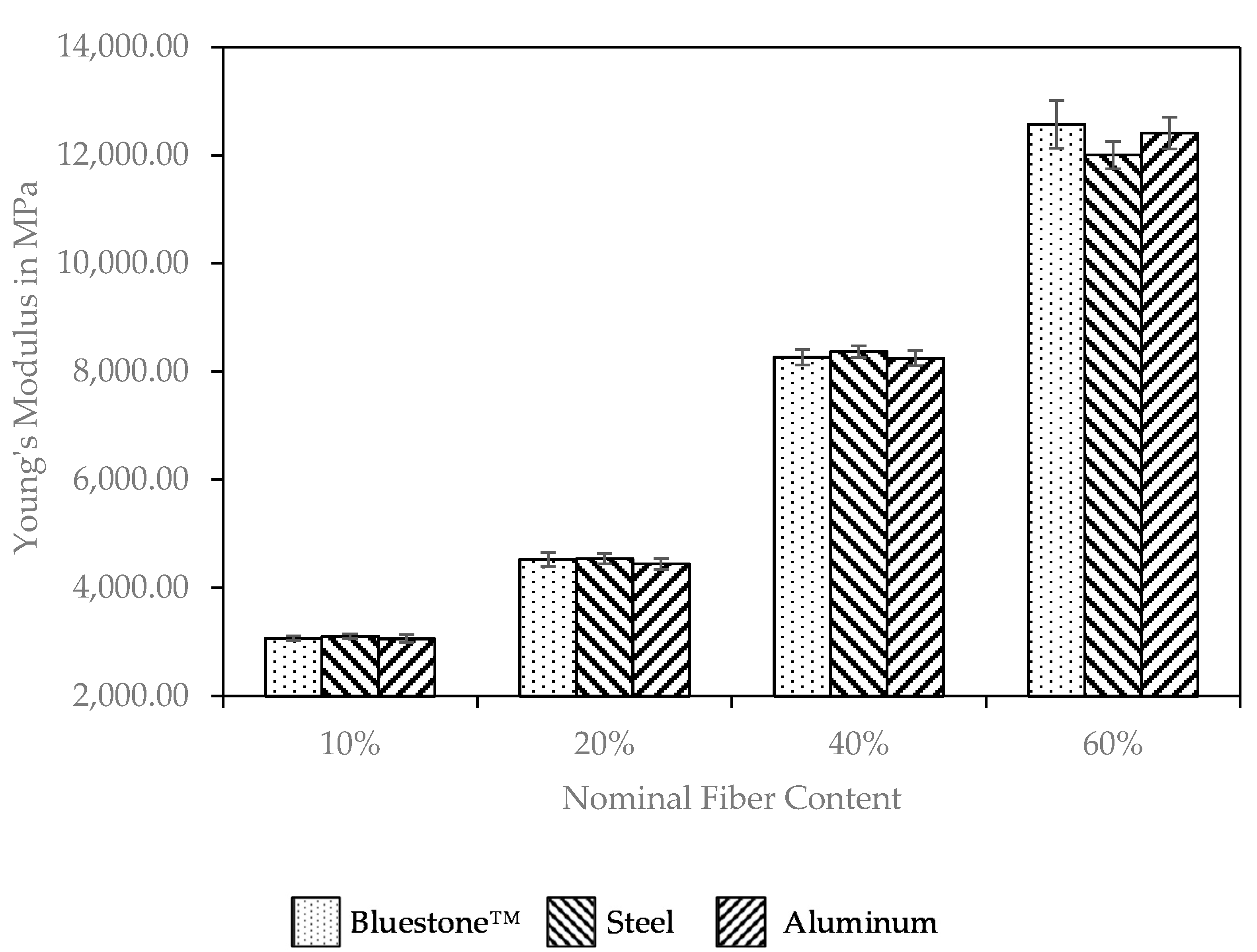
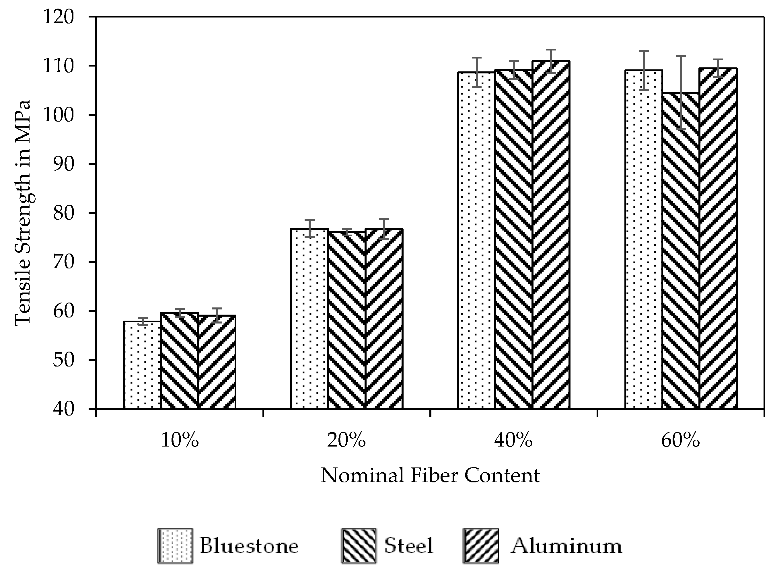
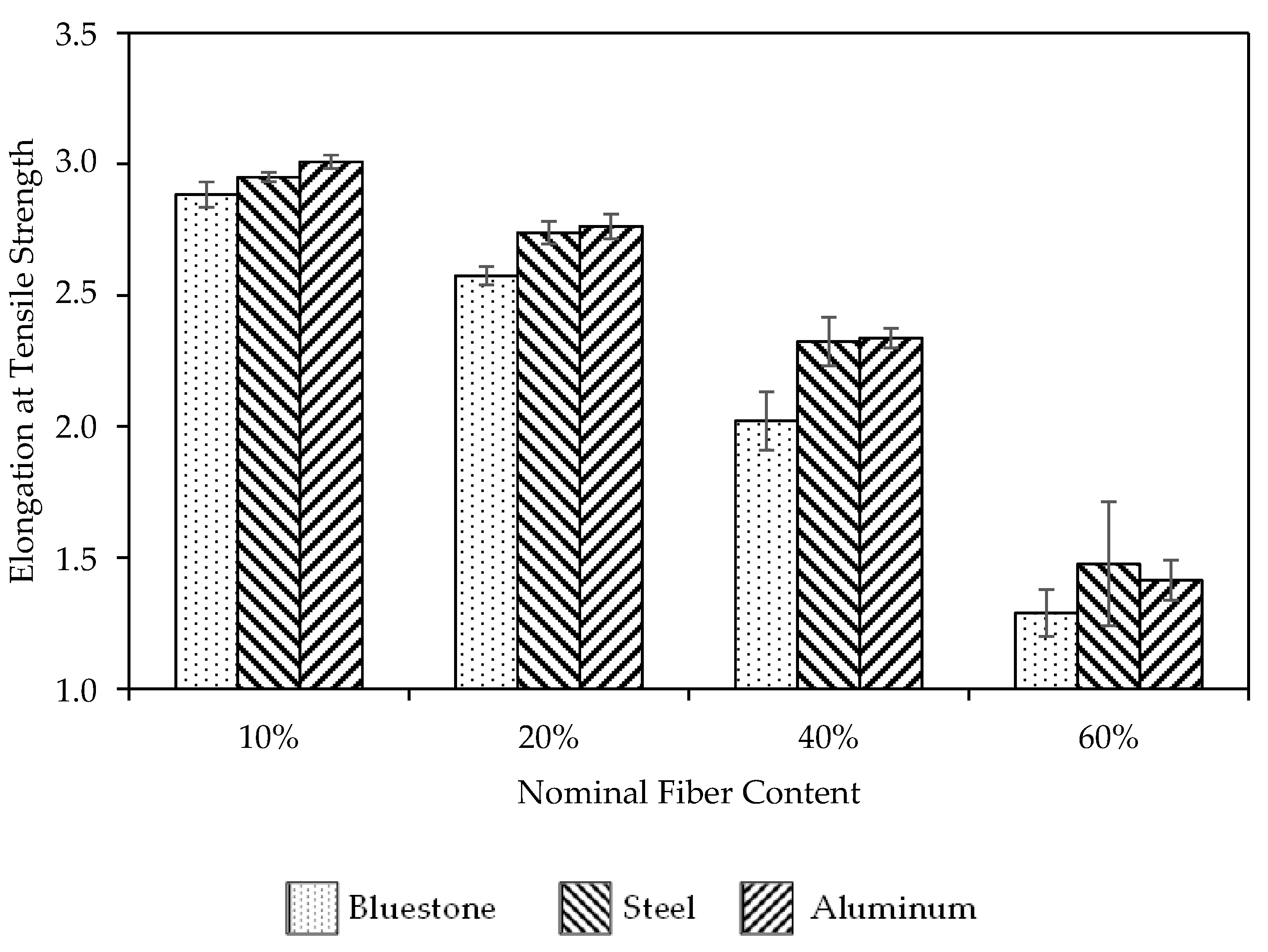
The objective of this investigation is to qualify additively manufactured polymer tools for the fabrication of LFT parts for functional validation, spare parts, and small series production. For this purpose, the effects of three different tool materials (ceramic reinforced plastic, steel, and aluminum) on the process-induced fiber configuration are investigated and compared with each other. The iterative tool design process is performed for all materials individually and is based on Moldflow simulations and basic principles of heat transfer. Especially in terms of the cooling systems, the advantages of AT are specifically implemented. Representative for the most used LFT, the glass fiber-reinforced PP injection molding material STAMAX™ from SABIC is used in different fiber weight percentages. Tensile specimens and discs are used as sample geometries to map both a linear and a radial source flow. The process-induced fiber configuration is investigated over the flow path and over the component thickness. The central injection point at the disc mold will also allow investigation of the transition from a swirling to a pointed flow. Furthermore, the impact of the different tool materials on significant mechanical properties of the fiber-reinforced moldings are analyzed. For the test methods, CT scan, pyrolysis, tensile testing, and a fiber length measurement method modeled after that of Goris et al. [
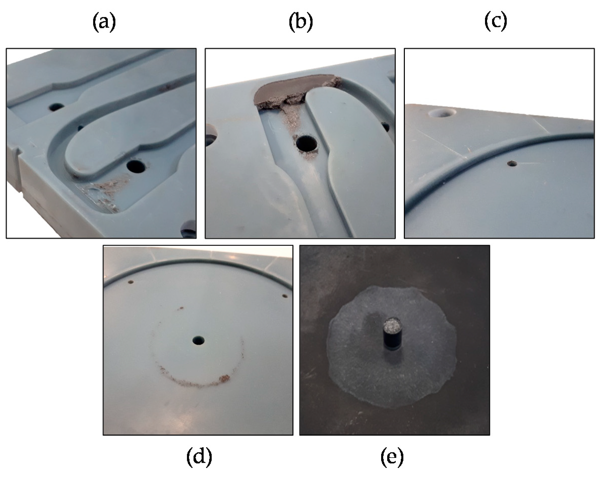
17] are carried out. To evaluate the economic efficiency, the tool life and the suitability of AT will be assessed on the degree of wear, defect patterns, and output quantity.

1.2. State of the Art

AM is ideally used to manufacture components directly without using the indirect process chain of AT. For this purpose, there are many commercially available fabrication methods (i.e., fused filament fabrication (FFF), selective laser sintering (SLS), and multi jet fusion) and materials that contain fiber reinforcements. However, their properties are not comparable with IM materials and especially not with LFTs due to their short fiber character and diverging fiber configuration. The commodity polymer PP is well known for its difficulty in processing within AM due to its shrinkage and low adhesion. Nevertheless, Sodeifian et al. [18] achieved good processing results of PP/GF with the additive POE-g-MA on a FFF platform. Still, the material is lagging behind in its mechanical properties and is deviating strongly from its compression molding pedant by 30%. To fabricate classic IM materials directly, another promising approach arose in the most recent decades. It is a modified FFF method where the filament extruder is exchanged for a granulate-fed portable extruder unit. On that base, Hertle et al. [19] achieved good results by melt extrusion of PP injection molding granulate. Though it was unlikely, the process suffers the same issue of an insufficient interlaminar bonding, which is strongly incoherent compared to the intralaminar ones and is leading into anisotropic material properties [20].
AT is the indirect process chain and a tool-bound alternative, which allows it to maintain the original manufacturing process and its material variety. Kampker et al. [21], investigated the suitability of polyjet (PJ), SL, digital light synthesis (DLS), and SLS processes for direct IM tool production. The investigations showed that the material PA 3200 GF is the most suitable for SLS, while for the SL method, composite materials such as Accura® Bluestone™ and Perform are the most promising ones. Rahmati and Dickens [22] examined the output of SL produced tools in the field of IM. They achieved an output of more than 500 parts and found that the main tool failure was due to flexural and excessive friction. Hofstätter et al. [23] achieved the same results.
For the improvement of the part properties, as well as the extension of the tool life and to decrease the cycle time, extensive research is being done on optimized cooling systems and adapted process parameters. Altaf et al. [24] demonstrate the general effectiveness of a conformal cooling system in a direct comparison with a conventional cooling design. In this example, the conformal cooling system leads to a cycle time reduction of approx. 20%. The investigations of Park et al. [25] show even better performances of up to 30%, whereby only tool areas relevant to the cycle time are replaced by SLM (Selective Laser Melting) inserts with a conformal cooling unit. However, Hopkins et al. [26] observed in a direct comparison of an aluminum and a polymer IM tool an increased cycle time and significant differences in the rheology of the injection molding material. The lower thermal conductivity of the mold materials results into longer flow paths, which in turn requires lower process pressures and melt temperatures. In earlier investigations of Martinho et al. [27], the influence on the morphology of semi-crystalline PP moldings is revealed in a direct comparison of an epoxy and steel mold material. As soon as different materials were used for core and cavity, a clear asymmetrical crystalline structure was observed. In concerns of the influence on the material properties of the moldings, the investigations of Harris et al. [28,29] should be emphasized. He states that with the aid of a modified cooling system and the adaptation of the necessary process parameters, the crystallinity can be strongly influenced, even to the extent that comparable part properties can be achieved using polymer and CNC milled steel/aluminum molds. Similar results were achieved by Fernandes et al. [30] and Volpato et al. [31]. Recent investigations by Kampkar et al. [16] proved that the materials still show a rather brittle and non-ductile fracture behavior. However, the deviations can be attributed with high probability to particle agglomeration due to the lower thermal conductivity and a greater surface roughness.
On the side of LFTs, the investigations of Kim et al. [32] show that the mechanical and the impact strength increases with the fiber length. Furthermore, they measured a reduction of the initial fiber length of 4–16 mm to a residual fiber length of about 0.5–2 mm during processing. The results are consistent with Seong et al. [33], who noted an increase in Young’s modulus, melting temperature, and viscoelastic properties, and a less uniform distribution of the fiber with an increasing fiber length. Hou et al. [
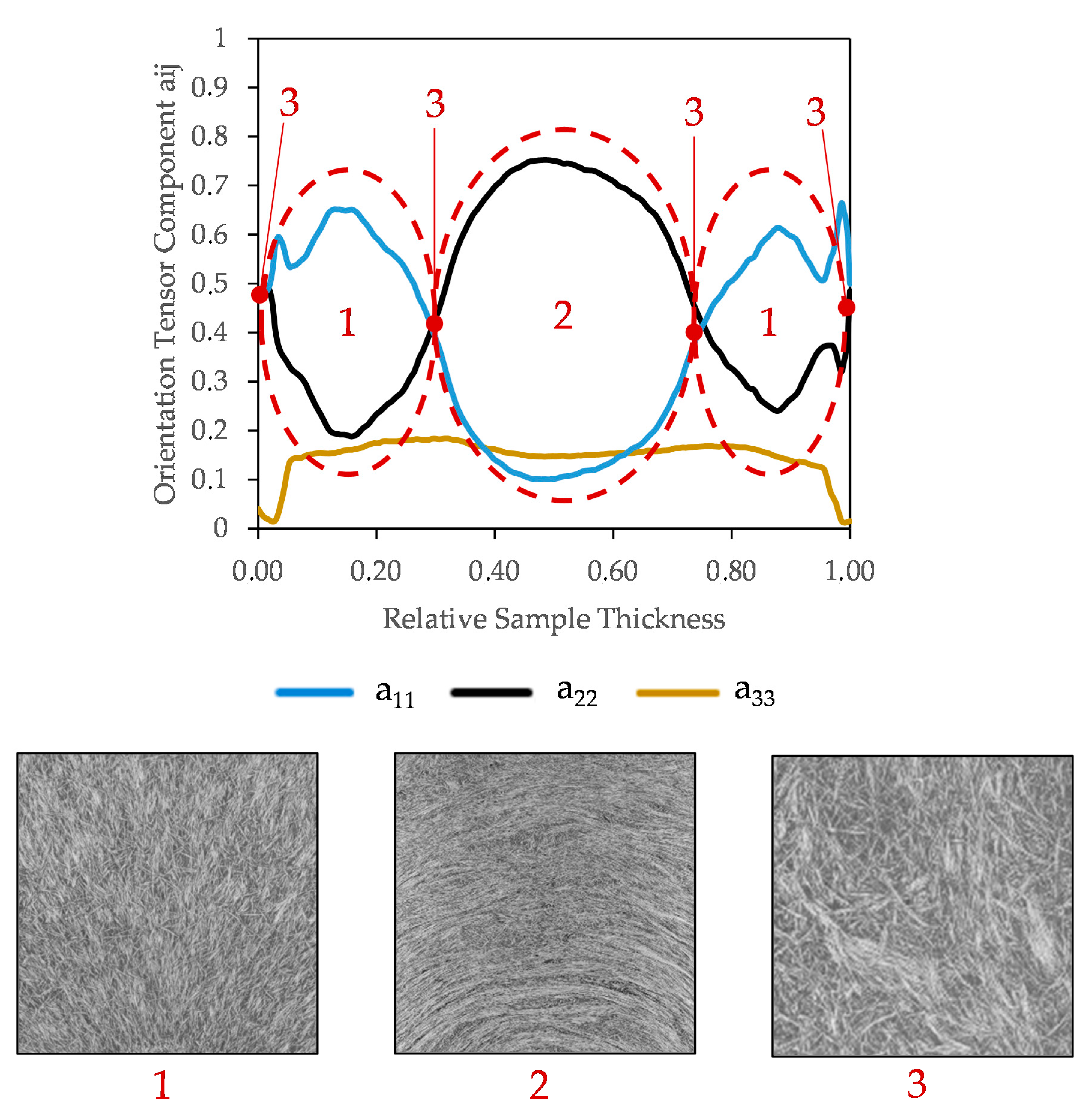
34] measured a reduction of the average fiber length with an increasing injection rate over the whole length of tensile specimens. Based on the work of Tadmor [35] as well as Osswald and Menges [36], there are seven characteristic regions that can be differentiated in injection molded parts, each with a specific fiber orientation. The two skin layers provide random fiber orientation, while the shell layers are aligned parallel to the melt flow direction. The fiber alignment of the core layer is perpendicular to the melt flow direction, with two randomly oriented transition layers between the core layer and the shell layers. This specific orientation pattern is well-known and caused by the fountain flow effect. However, the numerical predictions of Hou et al. [34] do not match with the empirical orientation in the skin layer. Parveen et al. [37] achieved comparable results to Hou et al. on a disc geometry (2 mm; 75 mm D) and stated that a higher fiber length leads to a wider core region with more fibers aligned transverse to the flow direction at the end of the flow path. Zhu et al. [38] compared a centered and an end-gated injecting model. It is found that the end-gated plate has a more defined shell area of 55%, where the fibers align along the main flow direction and a core region of 20%, with fibers aligned perpendicular to it. The shell area of the center-gated plates takes a 35% and the core area 35% at an equal density and fiber weight content. Goris et al. [17] detected a substantial increase in fiber length along the flow path, which is probably due to a fiber pullout effect. The same could be observed by Lafranche et al. [39], who detected a strong influence of the used gate type in addition. Furthermore, Goris [17] demonstrated in a comparative study that the so-called epoxy plug method, which is based on the investigations of Kunc et al. [40]. The new measurement method is especially suitable for LFTs with a large sample size and can be used to generate accurate results with a strong repeatability while minimizing the manual handling effort. It is shown that the taken measurements agree with the outcome of previously reported studies [12,39,41]. Aside from the epoxy plug method, the comparative study concentrated on two other fiber analysis methods: first, a full fiber analysis, which is a proprietary measurement system developed by SABIC (Geleen, Netherlands) and based on the work by Krasteva [42]; and second, the FASEP method, which is a commercially available analysis method proprietary to IDM Systems (Darmstadt, Germany).
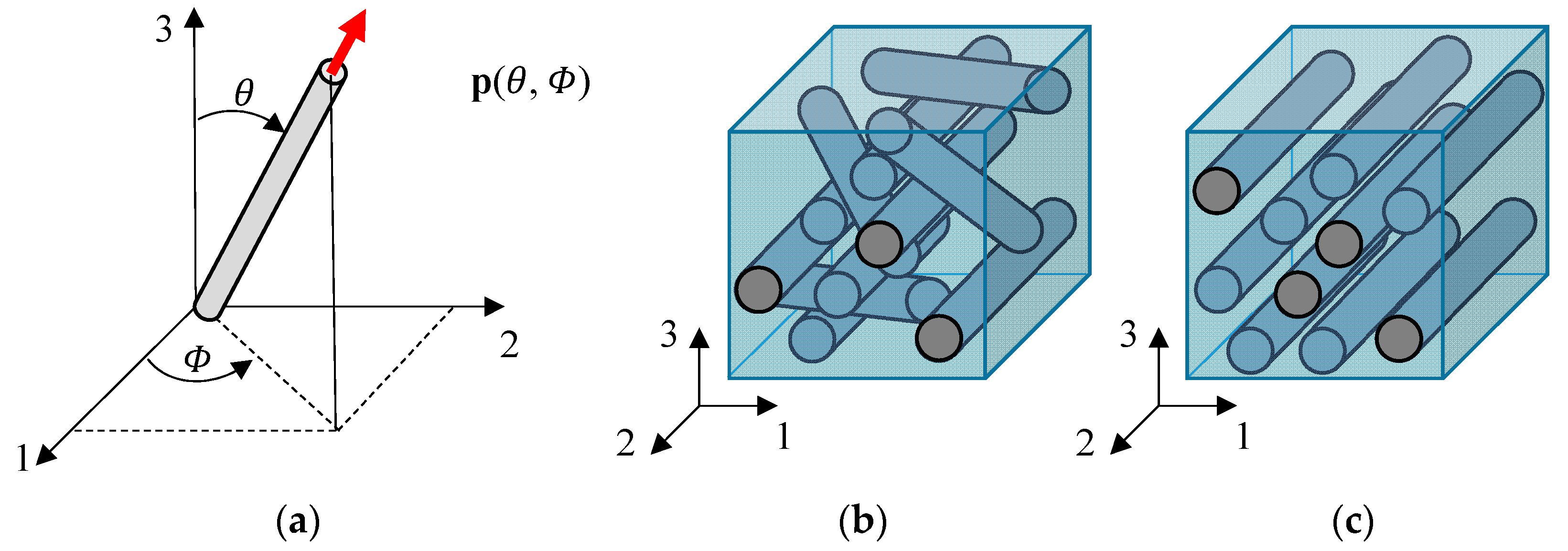
For the analysis of the fiber orientation distribution, Sharma et al. [43] achieved sufficient results with a tensor-based marker watershed method. However, the method is relatively sensitive to improper surface preparation and image processing techniques. A better application seems to be the evaluation of industrial micro-computed tomography (μCT) images. The fiber orientation is described in accordance with the work of Adavani and Tucker [44], who assume that each fiber can be represented by a unit vector p spherical coordinates. The orientation is then described in tensor form. A schematic representation can be seen in Figure 1 (left). Mathematically, the unit vector is described with the angles Φ , θ as:
p = ( p 1 p 2 p 3 ) = ( cos ( Φ ) · sin ( θ ) sin ( Φ ) · sin ( θ ) cos ( θ ) )
The orientation tensor or Advani–Tucker tensor is calculated as:
α i j = p i · p j · Ψ ( p )   d p
While p i · p j is the product of the fiber orientation vector with itself, Ψ ( p ) represents a probability function of all possible orientations. This results in the following tensor components:
a 11 = sin 2 ( Φ ) cos 2 ( θ ) a 12 = sin 2 ( Φ ) cos ( θ ) sin ( θ ) a 13 = sin ( Φ ) cos ( Φ ) cos ( θ ) a 21 = a 12 a 22 = sin 2 ( Φ ) sin 2 ( θ ) a 23 = sin ( Φ ) cos ( Φ ) sin ( θ ) a 31 = a 13 a 32 = a 23 a 33 = cos 2 ( Φ )
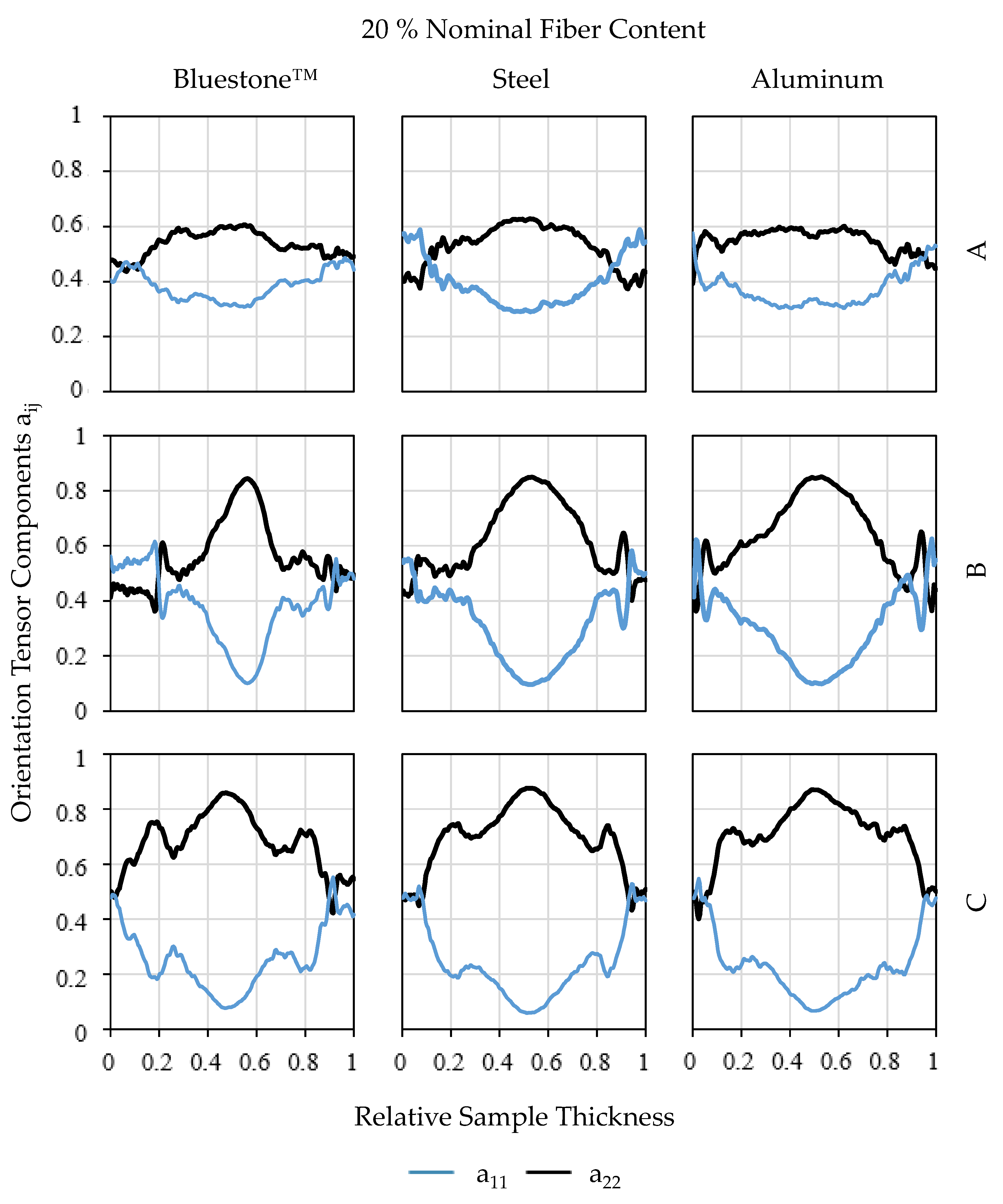
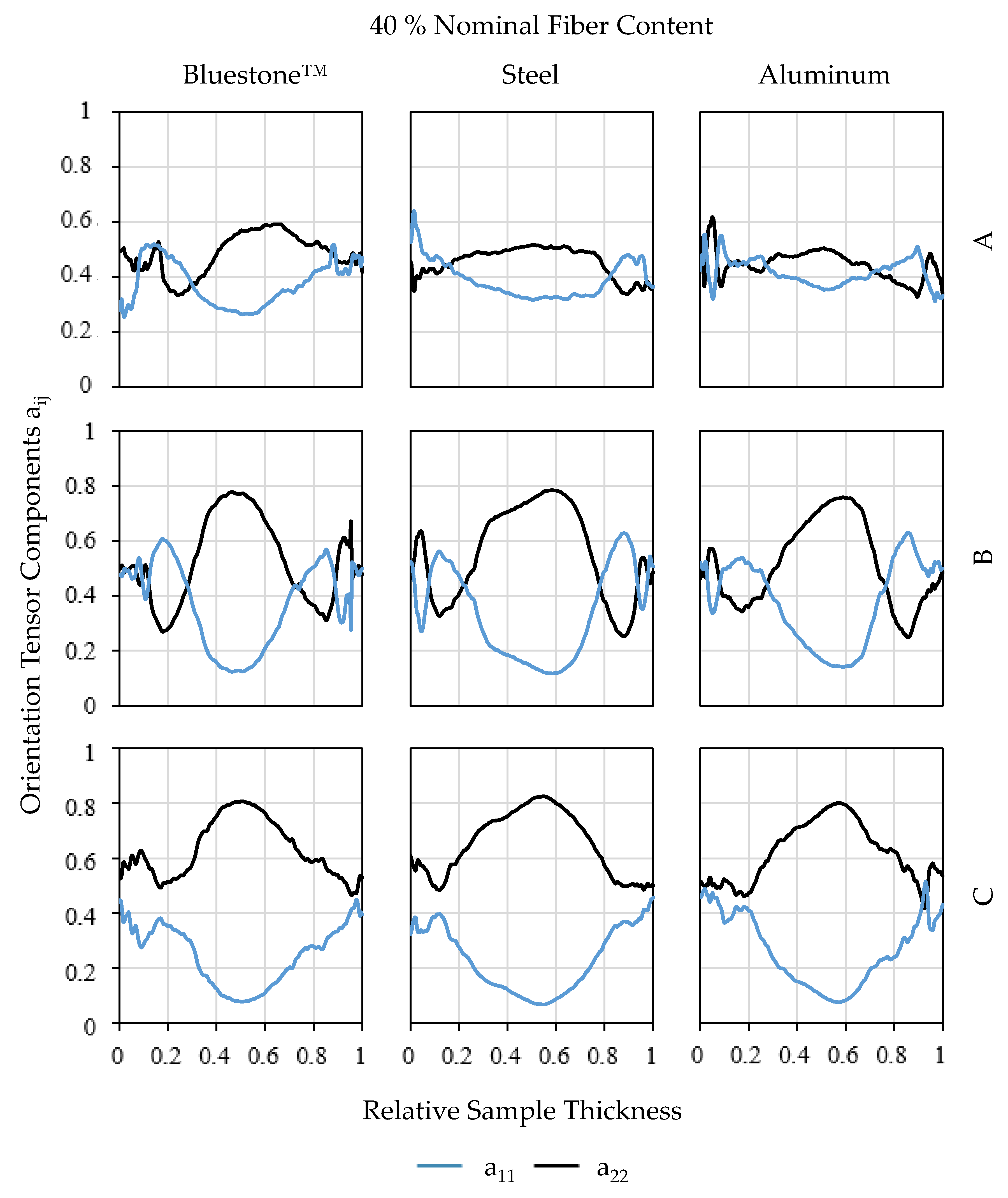
Experimental data are conventionally illustrated using the orientation tensor form. The diagonal components of the second order orientation tensor ( a 11 , a 22 , and a 33 ) describe the degree of orientation with respect to the defined coordinate system. Conventionally, the reference coordinates are defined so that the 1-direction represents the inflow direction, the 2-direction is the crossflow direction and the 3-direction is the thickness direction. The off-diagonal components of the orientation tensor show the tilt of the orientation tensor from the coordinate axes. Hence, they are zero only if the coordinate axes align with the principal directions of the orientation tensor [44]. Two examples for possible fiber alignment are given in Figure 1. If completely random orientation occurs, the diagonal elements are a 11 = a 22 = a 33 = 1/3 (middle). For fiber orientation perpendicular to in-flow direction, the tensor elements are a 11 = 0 a 22 = 1 and a 33 = 0 (right).

2. Materials and Methods

2.1. Materials and Specimens

2.1.1. Specimen Geometry and Mold Insert Design

The specimen geometries used in this work are shown in Figure 2. The test specimen geometry for tensile tests according to DIN EN ISO 527 is based on the multipurpose specimen geometry 1A according to DIN EN ISO 527-1 and DIN EN ISO 3167. For a high reproducibility of the specimen geometry, the cavity of the injection molding tool is flow-optimized in deviation to DIN ISO 294-1 to keep the wear of the AM tools as low as possible. The test specimen with its long flow path ratio is representative for a linear directed flow behavior. Due to the wall thickness of 4 mm, a good separation of a skin–shear–core–shear–skin orientation can be expected. The cavity and specimen geometry are shown in Figure 2.
For the investigation of the fiber configuration, a nonstandard disc with a thickness of 3 mm and a diameter of 120 mm is used. Due to the rotation symmetry of the disc, only a partial segment of the disc needs to be examined to draw conclusions about the entire test specimen. The central injection point at the disc mold will allow investigation of the transition from a swirling to a pointed flow. Likewise, a radial geometry provides an even pressure distribution during the IM process and thus reduces the process-induced influence on the test specimens and measurement results. This plays an important role especially for AM tools, which tend to have a high deformation and mold breathing. Furthermore, the disc geometry is frequently used in literature, so that the obtained results can be compared with existing studies of Hongyu and Baird [45]. In the cases of Rohde et al. [46] and Goris et al. [17], who focused more on a plate geometry, the results can be seen as complementary and further investigation. The cavity and specimen geometry are shown in Figure 3.

2.1.2. Materials

The AM tools are made from Accura Bluestone by the company 3D Systems®, which is processed on a Viper si2 System (SLA). Accura Bluestone is a ceramic filled epoxy composite, which is characterized by relatively high heat deflection temperature of up to 284 °C and a tensile strength about 8000 MPa [47]. Due to its material characteristics, high imaging accuracy and low surface roughness, Kampkar et al. [21] recommend Accura Bluestone as an AM tool material.
The thermal conductivity coefficient of Accura Bluestone was determined for this investigation at approximately 0.781 W/mK, which is 50 times lower than the thermal conductivity of conventional steel (34.5–49.3 W/mK) [48] and 150 of aluminum (130–160 W/mK) [49]. Aside from the cooling system, all other tools are identical in their geometry and design. Table 1 shows a brief comparison of the material properties of the different tool materials. As a reference, the same tools are conventionally milled from aluminum (EN AW-7075) and steel (C45 U).
To increase the heat deflection temperature, the Accura Bluestone mold insert is tempered with a temperature profile as recommended by 3D Systems. This is done through thermal post curing for 2 h at 120 °C, which increases the deflection temperature from 65–66 °C to 267–284 °C [47].
Representative for the most used LFT, the glass fiber-reinforced PP injection molding material STAMAX from SABIC is used in different fiber weight percentages of 10 wt.%, 20 wt.%, 40 wt.%, and 60 wt.%. The specific fiber contents are chosen in accordance with the results of Goris [50], which showed the highest contrast and a clear differentiation for interpretation. Ratios of 30 wt.% and 50 wt.% were not considered to keep the experimental volume adequate. STAMAX is a certified product series for the automotive industry and is already available pre-mixed in many different glass fiber contents. Accordingly, the mixing ratios 20 wt.%, 40 wt.%, and 60 wt.% for the investigations can be obtained directly. The mixing ratio 10 wt.% is gravimetrically prepared from STAMAX 20 wt.% (20YM240) and pure PP, which the manufacturer SABIC uses as a base matrix material. In addition to its wide industrial usage, the material is characterized by its particularly good processability. PP has a wide processing temperature range with a low melt viscosity, melt temperature, and adhesivity. This is beneficial to reduce the thermal and mechanical stress on the polymer tools and to ensure the possibility to produce enough samples for the evaluation. For the specimen fabrication, a Boy 25 E injection molding machine from Dr. Boy GmbH & Co. KG is chosen.

2.2. Experiment Methodolgy

2.2.1. Mechanical Properties

To analyze the mechanical properties, tensile testing after DIN EN ISO 527 is performed. The results are analyzed toward tensile strength, elongation, and Young’s modulus. For the calculation of the standard deviation, five samples of each specimen type are analyzed as recommended by DIN EN ISO 527. Nominal fiber contents of 10 wt.%, 20 wt.%, 40 wt.%, and 60 wt.% are analyzed. In accordance with DIN EN ISO 527, a testing speed of 1 mm/min is used for determination of the elastic properties and, more specifically, the determination of the Young’s modulus. For the deformation properties, the testing speed is increased to 50 mm/min for the practical purpose of decreasing testing time. Although not in accordance with the norm, this is a common approach in the field of tensile testing. However, this effect must be considered for the discussion of the test results.

2.2.2. Fiber Length Analysis: Epoxy Plug Method

The epoxy plug method is centered around a down-sampling step after Kunc [40], which reduces the fiber count from <1,000,000 to a representative amount around 15,000–60,000 fibers. The detailed experiments steps are depicted in Figure 4.
As can be seen in Figure 4, the matrix material of the sample is initially removed. A sample diameter of at least twice the initial fiber length must be chosen to avoid measuring fibers that crossed the cutting plane during extraction. An initial fiber length of 15 mm results in a diameter of 30 mm. The matrix removal is performed by pyrolysis at 500 °C for 8 h in an industrial oven. Rohde et al. [46] studied the impact of matrix removal by pyrolysis or chemical decomposition on the morphology of single fibers. The results show that performing pyrolysis at 500 °C for 2 h is optimal for a PP sample. However, initial test runs showed that the pyrolysis time needed to be extended to 8 h to sufficiently remove the matrix.
For this investigation, the selection of the experimental fiber analysis test method was based on two factors: to provide sufficient repeatability and comparability toward previous investigations, as well as being able to generate an adequate output with a reasonable experiment duration. Therefore, the developed method by Goris et al. [17] (compare Section 1.2) was chosen. Based on the investigations of Rohde et al. [46], a thermal matrix removal is chosen instead of a chemical removal, since the fiber length could be negatively altered. Next, the down-sampling step is performed. A defined amount of UV-activated epoxy B0027N07MM liquid-glue by the company BONDIC (Aurora, Canada) is injected in the exposed fiber bed. The diameter of the injected epoxy varies from ca. 4–7 mm. After UV-curing of the glue and careful removing of non-attached fibers, a second pyrolysis is performed at 500 °C for 8 h. The subsequent fiber dispersion step is performed within a dispersion chamber, which can be seen in Figure 5. The turbulent dispersion is performed through small amounts of pressured air, performed 3–4 times at 1 bar for around 0.5 s. The fibers are than dispersed on a 210 mm × 255 mm × 4 mm glass plate, which is positioned on an EPSON Perfection V800 Photo scanner of the company Seiko Epson (Suwa, Japan) to create a digital image at 2400 dpi. For image enhancement and threshold, Adobe® Photoshop™ is used. Threshold levels are approximately 40 at the image center and 60 at the edges. This variation is necessary due to inhomogeneous illumination. Then, a MATLAB-based algorithm is used for fiber detection, which was developed at the Polymer Engineering Center (Madison, WI, USA) [51] and is based on the work of Wang [52]. The fiber detection is automated and even detects stacked and bent fibers.
Two different averages are calculated for investigation of the fiber length: number average and length average. The number average is calculated using (compare nomenclature Table 2)
L N = i = 1 n ( N i · l i ) i = 1 n ( N i )
and the length average (compare nomenclature Table 2)
L W = i = 1 n ( N i · l i 2 ) i = 1 n ( N i · l i )
Long fibers have a more significant impact on the length average than short fibers. This effect is described as nonuniformity, of which high values are usually preferable in technical applications. Another effect that must be considered during the epoxy plug method is the preferred pickup of long fibers during the down-sampling step. This phenomenon can lead to a distorted average fiber length and is schematically represented in Figure 6. Five fibers are visible, from which only four are picked up by the down-sampling region. The fifth does not contribute to the experimental analysis aside from a similar alignment of the center of mass of each fiber. Therefore, Kunc et al. [40] introduced the so-called Kunc correction, which determines a corrected fiber frequency Ni in favor of shorter fibers. It is calculated as:
N ( L i ) = θ ( L i ) · ( 1 + 4 · L i π d )
For this investigation, the analysis of the fiber length focuses on the analysis of the fiber-reinforced discs. Three segments—A, B, and C—with a diameter of 30 mm ± 0.5 mm are therefore removed by sawing from discs as depicted in Figure 7. The diameter is chosen based on the initial fiber length of 15 mm for STAMAX pellets. For the calculation of the standard deviation, three samples were analyzed for each location. Nominal fiber contents of 10 wt.%, 20 wt.%, 40 wt.%, and 60 wt.% are analyzed.

2.2.3. Fiber Content Analysis: Pyrolysis

The analysis of the fiber content is determined gravimetrically. For this, a pyrolysis in accordance with DIN EN ISO 3451 is performed for each sample within an industrial oven. Each sample is kept at 100 °C for 30 min before the matrix is removed at 625 °C for 3 h. This represents a less gentle and therefore faster temperature program compared to the pyrolysis steps of the epoxy plug method, since the fiber quality is not important for this experiment. The fiber content is then calculated in accordance with DIN EN ISO 3451 as (compare nomenclature Table 3):
α = m F m T o t a l · 100   w t %
For this investigation, the analysis of the fiber content focuses on the analysis of the fiber-reinforced discs. The discs are therefore quartered and segmented in 33 squares with an edge length of 11.5 mm ± 0.5 mm as depicted in Figure 8. The samples were then cut out with scissors, resulting in 22 segments with identical in volume for each nominal fiber content, as well as 11 segments from the disc edges with varying volume and sample shape. The varying shape does not constitute a problem for later calculation of the fiber content, since the results are normalized by the individual total sample mass. For the calculation of the standard deviation, three samples were analyzed for each location. Nominal fiber contents of 10 wt.%, 20 wt.%, 40 wt.%, and 60 wt.% are analyzed.

2.2.4. Fiber Orientation Analysis: Micro-Computed Tomography

For fiber orientation analysis, μCT scans are used, which are performed with a GE v|tome|x m 240/180 by the company General Electric (Boston, MA, USA). The scan parameters can be seen in Table 4.
The analysis of the μCT data is performed with VGSTUDIO MAX 3.3.0 64 Bit by the company Volume graphics GmbH (Heidelberg, Germany). The software was chosen in accordance with a comparative study by Goris [17], which compared results of the conventional method of ellipses to μCT-data analyzed with three different algorithms: VGSTUDIO MAX 3.3.0 64 Bit, slit method (SM) algorithm, and Mimics (proprietary to SABIC and Materialise MV). The results showed that a minimal resolution of 19 ± 1 μm could be used to sufficiently analyze the fiber orientation using VGSTUDIO MAX. For this investigation, the analysis of isotropic fiber orientation is performed with plane projection. The direction of the normal vector is identical to the thickness direction. Table 5 shows the detailed analysis parameters. As can be seen, the fiber material is defined by specific threshold, which is identical for all samples.
For this investigation, the analysis of the fiber orientation focuses on the analysis of the fiber-reinforced discs. As depicted in Figure 9, a rectangular sample of 18 mm × 70 mm (±0.5 mm) is removed with a saw from each disc. Three squares—A, B, and C—with an edge length of 12 mm ± 0.5 mm are then analyzed within VGSTUDIO MAX. Nominal fiber contents of 10 wt.%, 20 wt.%, 40 wt.%, and 60 wt.% are analyzed. Due to limitations for the experimental amount, only one sample of each fiber content and tool type is analyzed.

2.3. Processing Parameters and Tool Design

The processing parameters for STAMAX are based on the processing guidelines [53] recommended by SABIC. Within these guidelines, a distinction is made between minimum, moderate, and maximum parameters. For this investigation, moderate parameters are targeted to generate comparability to the results of Goris [50]. In accordance with the guidelines, the injection pressure is chosen at 800 bar with linear decline down to 700 bar for steel tooling, with moderate injection speeds of 70 ccm/s to 60 ccm/s. The holding pressure is recommended at 50–80% of the injection pressure. Therefore, a holding pressure of 400 bar is chosen with a linear decline to 350 bar. Since aluminum and Bluestone provide lower mechanical properties than steel, the processing parameters including the clamping force for these tools were lowered accordingly. Table 6 gives a detailed overview of the processing parameters of each tooling type.
The melt temperature is chosen at 250 °C with a flat temperature profile within the screw cylinder. As can be seen, the mold temperature is set to 30 °C. The cooling process is accomplished through a water-cooling cycle of the same temperature. As soon as the implemented temperature sensors near the cavity reach the targeted temperature, a new cycle can be started.
As described before, geometrical limitations for the cooling channels are small due to additive manufacturing. This is represented in Figure 10, which shows the difference in possible cooling cycle alignment for ejector half metal disc tools (a) and additively manufactured disc tools (b).
As can be seen, sealing plugs were used to close the boreholes of the metal tools. For the fixed mold half, the cooling path is analogue to the ejector half. The cooling channel geometry was determined through iterative calculation steps based on fundamental theorems of heat transfer and through calculation of the divergence in mold temperature. Moldflow simulations were used to guarantee a homogenic average mold temperature of the developed concepts, to minimize the effect of different cooling channel geometries on the results. As an example, the simulative results of Bluestone tensile specimen-tools are depicted in Figure 11.
As can be seen, the average temperature ranges from approximately 30 °C up to 125 °C. The highest temperatures can be seen in the stagnation points of the melt at the tensile specimen shoulders. Since for Bluestone, a uniform temperature could not be guaranteed within the whole part, the focus lied on creating a homogenous average temperature within the functional regions, which is the gauge for tensile specimens. The stagnation points (red) were defined as critical regions, which will be discussed further in the following chapter. In case of the tensile specimens, parabolic runners with a diameter of 5 mm and a non-specified gate are used only on the ejector half. For the disc tools, the melt enters the cavity directly through the nozzle without the use of runners or a gate. The striking point of the melt also represents a critical region, especially for disc tools.

3. Results

3.1. Cycle Times Part Output and Failure-Modes

As can be seen in Figure 12, the recorded temperature near the critical region of tensile specimen Bluestone, aluminum, and steel tools are depicted. The final cycle times are determined through the critical mold temperature of 30 °C. As soon as the critical temperature is reached, a new cycle is started.
As can be seen, through the immense thermal conductivity of aluminum tools, the temperature in the depicted region fell even lower than 30 °C, close to room temperature, before a new cycle could be started. The results show that for every two Bluestone tool cycles, around seven steel cycles and eight aluminum cycles could be run. This directly translates to the increased thermal conductivity of steel and especially aluminum compared to Bluestone. In general, for every Bluestone tool type over 100 parts could be manufactured for all represented nominal fiber contents which includes tool trial runs. However, after a varying number of cycles depending on the tool type, different failure modes could be detected which were assessed as discard criteria or could be temporarily overhauled. The most prominent failure modes and deteriorations are depicted in Figure 13.
A typical challenge with additive manufactured components is the occurring staircase effect for steep geometries especially around angles of 45° paired with high temperatures. Figure 13 shows the critical regions with increased staircase effect (a), which caused demolishing of the mold especially at high fiber contents. For fiber contents of 60 wt.%, the demolishing eventually leads to clogging of channels at critical regions (Figure 13b). A typical deterioration for all nominal fiber contents is the abrasion of the mold material at the cavity edges (Figure 13c), which causes flashes on manufactured parts. This is either caused through underestimation of the clamping force, the flexibility of the mold or as an effect of repeated demolishing through material abrasion and heat exposure. A similar effect can be seen near the center of the mold and the melt entry point. After a non-specified number of cycles, these regions of high impact showed penetration of the mold through fibers and plain PP (Figure 13d). In extreme cases, the scraped mold material was found in the injected molded components (Figure 13e). Parts which showed signs of foreign particles and contamination were declared as rejects and the mold was eventually discarded. For aluminum and steel tools, none of the aforementioned failure modes or deteriorations could be detected.

3.2. Mechanical Properties

Generally, the results for the Young’s modulus (Figure 14) and the tensile strength (Figure 15) are increasing for rising nominal fiber contents, while the elongation at tensile strength (Figure 16) is declining. Typical for brittle materials, the elongation at tensile strength and the elongation at break are basically equal. The highest variation of the results is visible for nominal fiber contents of 60 wt.%.
The results of the Young’s modulus show that comparable values toward experimental data supported by the manufacturer are reached for every tool type and nominal fiber content. Furthermore, Bluestone tool specimens of 60 wt.% nominal fiber content are showing slightly higher values than steel and aluminum tools, although the increased variation of the results must be considered. An almost linear increase of the Young’s modulus can be detected with increasing nominal fiber contents, with maximum values around 12,000 MPa.
The results of the tensile strength also meet nearly identical values for each tool type and nominal fiber content. However, there is no detectable increase in tensile strength from 40 wt.% toward 60 wt.%, with maximum values around 110 MPa at 60 wt.%. As described before, the deformation analysis is performed at higher testing speeds than the analysis of the elastic behavior. This must be considered for the comparison of the tensile strength as well as the elongation at tensile strength toward the manufacturers’ data.
The elongation at tensile strength shows a constant decline toward higher nominal fiber contents since the material gets increasingly brittle. Aluminum and steel tools show almost identical results. However, test specimens of Bluestone tools show lower values than aluminum and steel tools, especially at nominal fiber contents of 40 wt.% and 60 wt.%. In further analysis, μCT data were able to show an increased number of voids for these nominal fiber contents, which are possibly caused due to limited processing conditions (Figure 17). The polymer matrix is responsible for an improved elongation behavior since stresses in lateral direction can be minimized. Through voids, the elongation and elastic behaviors are locally reduced.

3.3. Fiber Length

The results of the fiber length analysis for a nominal fiber content of 40 wt.% are shown in Figure 18. All other results for 10 wt.%, 20 wt.%, and 60 wt.% are represented in Appendix A. Analogue to the results of Goris [17] for steel tools, the length average of the fiber length reduces with increasing nominal fiber contents. The same phenomenon is visible for aluminum and Bluestone tools. Processing causes severe fiber breakage, which causes the number of long fibers to reduce. With increasing fiber contents, the shear stress and fiber interlocking increases, which causes increased early state fiber breakage. Therefore, the reached average values are far below the initial fiber length of 15 mm, with higher values for the length average compared to the number average. The highest length average variations are visible close to the gate and the entry point of the melt (Location A). This is most prominently visible for steel and aluminum tools at all nominal fiber contents. A possible explanation is the highly disoriented state in which the melt enters the cavity, thus creating a broader variety in fiber length. This theory can be further supported by the length average values, which show higher varieties than number average values. As described before, the length average values tend to be more highly impacted by the existence of a small number of relatively long fibers.
Depending on the locations A, B, and C, the depicted fiber contents show different behaviors with an increasing melt path. In general, the length average values of each tool type show higher fluctuations over the melt path than the number average values, which show a nearly stable length around 0.6 mm for all nominal fiber contents and tool types. This value directly translates to the results of Kim et al. [32], who declared a fiber length between 0.5–2 mm as typical values for long fibers after injection molding processing. Prominently stable results for the length average of each location are visible for Bluestone tools at nominal fiber contents of 40 wt.% and 60 wt.%, with a slight increase over the melt path (location A to C). Steel and aluminum tools show contrarian behaviors for nominal fiber contents of 40 wt.% and 60 wt.%, with maximum values at location A, followed by a decrease over location B to C. For a nominal fiber content of 10 wt.%, the samples of Bluestone tools show a decline in length average from location A to B, while increasing to maximum values of around 1.8 mm in location C. This behavior is also present for steel and aluminum tools, although to a lesser extent and with maximum values for the length average at location A. For 20 wt.% nominal fiber content, samples of Bluestone tools show contrarian behavior compared to 10 wt.%, with high length average values at locations A and B and a prominent decline in location C. A similar behavior is visible for aluminum tool samples, while samples from steel tools show almost identical behavior for 20 wt.% compared to 10 wt.%.
Despite the discussed differences in length average for different tool types, the results show that globally similar values for the average fiber length are reached depending of each tool material. Therefore, Bluestone tools can be declared viable for the use in functional validation of steel tools.

3.4. Fiber Concentration

The results of the fiber content analysis for a nominal fiber content of 40 wt.% are shown in Figure 19. All results for 10 wt.%, 20 wt.%, 40 wt.%, and 60 wt.% are represented in Figure 20. The schematic results for 10 wt.%, 20 wt.%, and 60 wt.% are shown in Appendix A. As can be seen, Figure 19 schematically depicts the results for an initial nominal fiber content of 40 wt.%, which show a characteristic increase in fiber content for all three tool types. This phenomenon can be seen for all initial nominal fiber contents. The lowest fiber concentration can be seen around the disc center with values mostly below and around the initial nominal fiber concentration. With increasing flow path, the fiber content increases until reaching above average values within the disc edges. This general increase of the fiber content with increasing melt path is visible for all nominal fiber contents, which is identical to the results of Goris [50]. A possible hypothesis for this behavior is the increase of the shear stress between liquid melt and solidified regions. Two effects occur in these regions: fiber breakage and fiber pullout. Through shear forces in the border region, the fibers are carried away by the melt flow and are shortened in this process. In retrospective to the results of the fiber length in Section 3.3, this phenomenon is especially visible on aluminum and steel tools. However, the results of Section 3.3 often show a limited or contrarian fiber shortening behavior for Bluestone tools toward metal tools. This is possibly caused by the slowed solidification and cooling process, as well as the limited processing conditions for Bluestone (injection speed, pressure, and clamping force). The fibers are more likely to be pulled out and carried off, with limited fiber breakage due to a more gradually transition between solidified material and the flowing liquid melt.
The comparison between Bluestone tools and steel tools for all initial fiber contents is represented in Figure 20. For the comparison of steel and aluminum tools, see Appendix A. As can be seen, for an initial nominal fiber content of 10 wt.%, the overall values for Bluestone tool samples are below the values of steel tools. This can most likely be explained through inaccuracy in the before discussed gravimetric mixture of equal parts 20 wt.% fiber-reinforced PP and plain PP. Regarding this, Bluestone tools and steel tools show nearly identical values and behaviors up to 40 wt.% initial nominal fiber content, with low standard variation. 60 wt.% samples from Bluestone tools show a higher spread toward minimum and maximum values compared to steel tools. This phenomenon is possibly caused by the gentler processing conditions for Bluestone tools. In comparison to the results of aluminum tools (see Appendix A), the results show that the best representation of steel tools for functional validation is through aluminum tools. However, the global fluctuation of the Bluestone tool samples is still low enough to be declared viable for functional validation of steel tools, especially for fiber contents up to 40 wt.%. The characteristic zones are identical for all tool types.

3.5. Fiber Orientation

As described in Section 1.2, seven characteristic regions can be determined in injection molded parts. Figure 21 shows the orientation tensor components over the relative sample thickness exemplified for a nominal fiber content of 60 wt.% at location B of a Bluestone tool specimen segment (in accordance with Figure 9). As can be seen, the characteristic zones can be identified (1, 2 and 3).
In addition to the identification of the characteristic zones, it is visible that the tensor component a 33 is constant over the entire relative sample thickness. This is valid for all examined segments. For further analysis of the fiber orientation, only components a 11 and a 22 are described because of their relevance toward the identification of the characteristic zones. Figure 22 shows the results for a nominal fiber content of 60 wt.% for Bluestone tools, steel tools and aluminum tools at locations A, B, and C. The results of all other nominal fiber contents can be seen in Appendix A.
As can be seen, the quality of the results is highly dependent on the sample location. Since B provides the most developed, unhindered, and oriented state of the melt flow, the characteristic zones are identifiable without further complication. Location A provides the most inconsistent transitions compared to locations B and C. A possible explanation for this behavior can be given based on the melt flow state. Since the melt flow is in a highly disoriented state when it enters the cavity, it is most likely that this region shows the highest inconsistencies toward fiber orientation. This behavior is present for all tool types and nominal fiber contents. Location C shows more consistent results than location A. However, due to the material stagnation at the edges of the disc, slight inconsistencies that hinder clear identification of the characteristic zones are still visible. Therefore, the decision was made to concentrate on location B entirely for the identification of specific trends dependent on increasing nominal fiber content, as well as different tool materials. The results can be seen in Figure 23.
It can be seen that there is a global increase of the shell layer thickness with increasing nominal fiber contents. A possible hypothesis for this phenomenon is based on different crystallization behavior for increasing fiber contents. Each fiber in the melt acts as a nucleating agent during cooldown. When more fibers are included, the crystallization process and solidification take place faster, which benefits increasing shell thickness. In terms of applicability for functional validation of steel tools, the Bluestone tools show almost identical fiber orientation compared to steel and aluminum tools. The thickness of the specific zones and the range of the orientation tensors are almost identical for all used tool types, which is essential for the qualification of Bluestone tools for functional validation. However, further repeated experiments are necessary for a sufficient qualification, since only one specimen of each tool type and nominal fiber content was examined during the experiments. Furthermore, the different thermal conductivities of all tool types impact the viscosity of the melt, which must be analyzed to solidify the aforementioned hypothesis.

4. Discussion & Conclusions

The discussion of the results of this investigation concentrates on two different aspects:
(a)
The general identification of characteristic phenomena dependent on the type of tool material and the nominal fiber content.
(b)
The relevance of the results toward the overall target, to use additively manufactured Bluestone tools as an alternative for steel tools for spare part and small series productions, as well as for the functional validation of steel tools.
The results of this investigation successfully illustrate, that specimens manufactured with Bluestone tools show comparable results toward metal tools for the mechanical properties and the fiber configuration, which includes fiber length, fiber concentration, and fiber orientation. In terms of the cycle times, the part output and the tool durability, Bluestone tools are not able compete with metal tools. As expected, zones of high impact and choke points proof to be critical for the Bluestone tool durability. A possible solution would be the use of modular concepts that make use of overall usable metal inlets, which can be applied at highly stressed regions. However, for the use of Bluestone tools in spare part and small series production, the reached part output of over 100 parts proves to be sufficient. Due to the similarity in fiber configuration and the mechanical properties, the use of Bluestone tools for functional validation is nearly qualified. Further experiments toward the fiber orientation need to be conducted to solidify the existing results.
Multiple characteristic phenomena could be detected, which are applicable for polymer tools, aluminum tools, and steel tools. For all tool types, the extent of the nominal fiber content influences two aspects: the thickness of the characteristic zones defined by Osswald and Menges [36], as well as the fiber length average. The analysis of the fiber orientation shows that with increasing nominal fiber content, the thickness of the shell layers increases respectively, while the thickness of the core layer decreases. A possible hypothesis for this phenomenon is based on the altered crystallization mechanism for increasing fiber contents. When more fibers are included, the crystallization process and solidification take place faster, which benefits increasing shell thickness. The analysis of the fiber length illustrates that the length average for specimens of each tool material decreases with increasing nominal fiber contents. The number average stays nearly stable for all tool types around 0.6 mm. This value directly translates to the results of Kim et al. [32], which declared a fiber length between 0.5–2 mm as typical values for long fibers after injection molding processing. Another phenomenon is determined through the analysis of the fiber concentration. Analogous to the results for rectangular specimens created through steel tools described by Goris [50], a gradual decrease of the fiber content is visible with increasing melt flow distance. This behavior is visible for steel tool specimens and now for Bluestone tool and aluminum tool specimens as well. A characteristic maximum at the edges of the disc specimens can be declared.
All in all, additively manufactured Bluestone proofs to be a viable approach for the rapid creation of polymer tools for injection molding processing. Further investigations will be centered around the improvement of the polymer tool lifecycle, as well as improved cycle times through efficient cooling methods. The use of modular concepts that make use of overall usable metal inlets needs to be further investigated. At last, the cost efficiency of polymer tools toward metal tools needs to be analyzed for a specific example in a comparative study.

Author Contributions

This investigation is based in equal parts on the scientific work of L.K. and R.S., under the supervision of D.R., K.W. and T.O. The work was divided in the following categories: Conceptualization, L.K.; methodology, L.K. and R.S.; software, L.K. and R.S.; validation, L.K. and R.S.; formal analysis, L.K. and R.S.; investigation, L.K. and R.S.; data curation, L.K. and R.S.; writing—original draft preparation, L.K. and R.S.; writing—review and editing, L.K. and R.S.; visualization, L.K. and R.S.; supervision, D.R., K.W., T.O.; project administration, L.K.; funding acquisition, no additional/external funding. All authors have read and agreed to the published version of the manuscript.

Funding

This research received no external funding. The APC was funded by Polymer Engineering Center, University of Wisconsin-Madison, Madison, WI 53706, USA.

Conflicts of Interest

The authors declare there is no conflict of interest.

Appendix A

Figure A1. Orientation tensor components ( a 11 , a 22 ; without a 33 for better overview) and relative sample thickness for a nominal fiber content of 10 wt.%. Specimens were created with Bluestone, steel, and aluminum tools, with samples from regions A, B, and C (in accordance with Figure 9).
Jcs 04 00136 g0a1
Figure A2. Orientation tensor components ( a 11 , a 22 ; without a 33 for better overview) and relative sample thickness for a nominal fiber content of 20 wt.%. Specimens were created with Bluestone, steel, and aluminum tools, with samples from regions A, B, and C (in accordance with Figure 9).
Jcs 04 00136 g0a2
Figure A3. Orientation tensor components ( a 11 , a 22 ; without a 33 for better overview) and relative sample thickness for a nominal fiber content of 40 wt.%. Specimens were created with Bluestone, steel, and aluminum tools, with samples from regions A, B, and C (in accordance with Figure 9).
Jcs 04 00136 g0a3
Figure A4. Fiber length (N = number average; W = weight or length average) for different tool types (for better representation in two diagrams) with 10 wt.% nominal fiber content at different specimen locations A, B, and C in accordance with Figure 7.
Jcs 04 00136 g0a4
Figure A5. Fiber length (N = number average; W = weight or length average) for different tool types (for better representation in two diagrams) with 20 wt.% nominal fiber content at different specimen locations A, B, and C in accordance with Figure 7.
Jcs 04 00136 g0a5
Figure A6. Fiber length (N = number average; W = weight or length average) for different tool types (for better representation in two diagrams) with 60 wt.% nominal fiber content at different specimen locations A, B, and C in accordance with Figure 7.
Jcs 04 00136 g0a6
Figure A7. Characteristic fiber content distribution pattern for disc segments of 10 wt.%, 20 wt.%, and 60 wt.% initial nominal fiber content: steel tool (a), Bluestone tool (b), and aluminum tool (c). The color scheme describes values below (blue) up to values near (white) and values above (red) the initial nominal fiber content (in accordance with Figure 8).
Jcs 04 00136 g0a7
Figure A8. Fiber content distribution for disc segments of 10, 20, 40, and 60 wt.% initial nominal fiber content at different locations (1–33 in accordance with Figure 7) for steel tools and aluminum tools.
Jcs 04 00136 g0a8

References

  1. Schemme, M. LFT—Development status and perspectives. Reinf. Plast. 2008, 52, 32–39. [Google Scholar] [CrossRef]
  2. Henning, F.; Ernst, H.; Brüssel, R. LFTs for automotive applications. Reinf. Plast. 2005, 49, 24–33. [Google Scholar] [CrossRef]
  3. Markets and Markets Research Private Ltd. Long Fiber Thermoplastics Market by Resin (PP, PA, PEEK, PPA), Fiber (Glass, Carbon), Manufacturing Process (Injection Molding, Pultrusion, D-LFT), End-Use Industry (Automotive, Electrical & Electronics), Region-Global Forecast to 2025; Markets and Markets Research Private Ltd.: Magarpatta, India, 2020. [Google Scholar]
  4. Markarian, J. Long fibre reinforcement drives automotive market forward. Plast. Addit. Compd. 2005, 7, 24–29. [Google Scholar] [CrossRef]
  5. Gómez-Monterde, J.; Sánchez-Soto, M.; Maspoch, M.L. Microcellular PP/GF composites: Morphological, mechanical and fracture characterization. Compos. Part A Appl. Sci. Manuf. 2018, 104, 1–13. [Google Scholar] [CrossRef]
  6. SmartTech Analysis. Additive Manufacturing Market Outlook and Summary of Opportunities; SmartTech Analysis: Charlottesville, VA, USA, 2019. [Google Scholar]
  7. Ngo, T.; Kashani, A.; Imbalzano, G.; Nguyen, Q.; Hui, D. Additive manufacturing (3D printing): A review of materials, methods, applications and challenges. Compos. Part B Eng. 2018, 143, 172–196. [Google Scholar] [CrossRef]
  8. Shaffer, S.; Yang, K.; Vargas, J.; Di Prima, M.; Voit, W. On reducing anisotropy in 3D printed polymers via ionizing radiation. Polymer 2014, 55, 5969–5979. [Google Scholar] [CrossRef]
  9. Zou, R.; Xia, Y.; Liu, S.; Hu, P.; Hou, W.; Hu, Q.; Shan, C. Isotropic and anisotropic elasticity and yielding of 3D printed material. Compos. Part B Eng. 2016, 99, 506–513. [Google Scholar] [CrossRef]
  10. Valino, A.D.; Dizon, J.R.C.; Espera, A.H., Jr.; Chen, Q.; Messman, J.; Advincula, R.C. Advances in 3D printing of thermoplastic polymer composites and nanocomposites. Prog. Polym. Sci. 2019, 98, 101162. [Google Scholar] [CrossRef]
  11. Achillas, C.; Tzetzis, D.; Raimondo, M.O. Alternative production strategies based on the comparison of additive and traditional manufacturing technologies. Int. J. Prod. Res. 2017, 55, 1–13. [Google Scholar] [CrossRef]
  12. Rohde, J.; Jahnke, U.; Lindemann, C.; Kruse, A.; Koch, R. Standardised product development for technology integration of additive manufacturing. Virtual Phys. Prototyp. 2018, 14, 141–147. [Google Scholar] [CrossRef]
  13. Wu, T.; Jahan, S.A.; Kumaar, P.; Tovar, A.; El-Mounayri, H.; Zhang, Y.; Zhang, J.; Acheson, D.; Brand, K.; Nalim, R. A framework for optimizing the design of injection molds with conformal cooling for additive manufacturing. Procedia Manuf. 2015, 1, 404–415. [Google Scholar] [CrossRef] [Green Version]
  14. Maravola, M.; Conner, B.; Walker, J.; Cortes, P. Epoxy infiltrated 3D printed ceramics for composite tooling applications. Addit. Manuf. 2019, 25, 59–63. [Google Scholar] [CrossRef]
  15. Yuan, S.; Shen, F.; Chua, C.K.; Zhou, K. Polymeric composites for powder-based additive manufacturing: Materials and applications. Prog. Polym. Sci. 2019, 91, 141–168. [Google Scholar] [CrossRef]
  16. Kampker, A.; Triebs, J.; Kawollek, S.; Ayvaz, P.; Beyer, T. Direct polymer additive tooling—Effect of additive manufactured polymer tools on part material properties for injection moulding. Rapid Prototyp. J. 2019. [Google Scholar] [CrossRef]
  17. Goris, S.; Back, T.; Yanev, A.; Brands, D.; Drummer, D.; Osswald, T.A. A novel fiber length measurement technique for discontinuous fiber-reinforced composites: A comparative study with existing methods. Polym. Compos. 2017, 39, 4058–4070. [Google Scholar] [CrossRef]
  18. Sodeifian, G.; Ghaseminejad, S.; Yousefi, A.A. Preparation of polypropylene/short glass fiber composite as Fused Deposition Modeling (FDM) filament. Results Phys. 2019, 12, 205–222. [Google Scholar] [CrossRef]
  19. Hertle, S.; Drexler, M.; Drummer, D. Additive manufacturing of poly(propylene) by means of melt extrusion. Macromol. Mater. Eng. 2016, 301, 1482–1493. [Google Scholar] [CrossRef]
  20. Mulholland, T.; Goris, S.; Boxleitner, J.; Osswald, T.; Rudolph, N. Process-induced fiber orientation in fused filament fabrication. J. Compos. Sci. 2018, 2, 45. [Google Scholar] [CrossRef] [Green Version]
  21. Kampker, A.; Triebs, J.; Ford, B.A.; Kawollek, S.; Ayvaz, P. Potential analysis of additive manufacturing technologies for fabrication of polymer tools for injection moulding—A comparative study. In Proceedings of the 2018 IEEE International Conference on Advanced Manufacturing, Yunlin, Taiwan, 16–18 November 2018. [Google Scholar]
  22. Rahmati, S.; Dickens, P. Rapid tooling analysis of stereolithography injection mould tooling. Int. J. Mach. Tools Manuf. 2007, 47, 740–747. [Google Scholar] [CrossRef]
  23. Summer Topical Meeting; American Society for Precision Engineering; European Society for Precision Engineering; Nanotechnology. Dimensional accuracy and surface finish in additive manufacturing. In Proceedings of the ASPE—The American Society for Precision Engineering, Raleigh, NC, USA, 27–30 June 2016. [Google Scholar]
  24. Altaf, K.; Rani, A.M.A.; Raghavan, V.R. Prototype production and experimental analysis for circular and profiled conformal cooling channels in aluminium filled epoxy injection mould tools. Rapid Prototyp. J. 2013, 19, 220–229. [Google Scholar] [CrossRef]
  25. Park, H.S.; Dang, X.-P. Development of a smart plastic injection mold with conformal cooling channels. Procedia Manuf. 2017, 10, 48–59. [Google Scholar] [CrossRef]
  26. Hopkinson, N.; Dickens, P. A comparison between stereolithography and aluminium injection moulding tooling. Rapid Prototyp. J. 2000, 6, 253–258. [Google Scholar] [CrossRef] [Green Version]
  27. Martinho, P.G.; Bartolo, P.J.; Pouzada, A. Hybrid moulds: Effect of the moulding blocks on the morphology and dimensional properties. Rapid Prototyp. J. 2009, 15, 71–82. [Google Scholar] [CrossRef]
  28. Harris, R.; Fouchal, F.; Hague, R.; Dickens, P. Quantifying part irregularities and subsequent morphology manipulation in stereolithography plastic injection moulding. Plast. Rubber Compos. 2004, 33, 92–98. [Google Scholar] [CrossRef] [Green Version]
  29. Harris, R.A.; Hague, R.J.; Dickens, P.M. Crystallinity control in parts produced from stereolithography injection mould tooling. Proc. Inst. Mech. Eng. Part L J. Mater. Des. Appl. 2003, 217, 269–276. [Google Scholar] [CrossRef]
  30. Fernandes, A.D.C.; De Souza, A.F.; Howarth, J.L.L. Mechanical and dimensional characterisation of polypropylene injection moulded parts in epoxy resin/aluminium inserts for rapid tooling. Int. J. Mater. Prod. Technol. 2016, 52, 37. [Google Scholar] [CrossRef]
  31. Volpato, N.; Solis, D.M.; Costa, C.A. An analysis of digital ABS as a rapid tooling material for polymer injection moulding. Int. J. Mater. Prod. Technol. 2016, 52. [Google Scholar] [CrossRef]
  32. Kim, Y.; Park, O.O. Effect of fiber length on mechanical properties of injection molded long-fiber-reinforced thermoplastics. Macromol. Res. 2020, 28, 1–12. [Google Scholar] [CrossRef]
  33. Seong, D.G.; Kang, C.; Pak, S.Y.; Kim, C.H.; Song, Y.S. Influence of fiber length and its distribution in three phase poly(propylene) composites. Compos. Part B Eng. 2019, 168, 218–225. [Google Scholar] [CrossRef]
  34. Hou, X.; Chen, X.; Liu, B.; Chen, S.; Li, H.; Cao, W. Fracture and orientation of long-glass-fiber-reinforced polypropylene during injection molding. Polym. Eng. Sci. 2020, 60, 13–21. [Google Scholar] [CrossRef]
  35. Tadmor, Z. Molecular orientation in injection molding. J. Appl. Polym. Sci. 1974, 18, 1753–1772. [Google Scholar] [CrossRef]
  36. Osswald, T.A. Understanding Polymer Processing: Processes and Governing Equations; Hanser Publications: Munich, Germany, 2017. [Google Scholar]
  37. Parveeen, B.; Caton-Rose, P.; Costa, F.; Jin, X.; Hine, P. Study of injection moulded long glass fibre-reinforced polypropylene and the effect on the fibre length and orientation distribution. AIP Conf. Proc. 2014, 1593, 432–435. [Google Scholar]
  38. Zhu, H.; Gu, Y.; Yang, Z.; Li, Q.; Li, M.; Wang, S.; Zhang, Z. Fiber distribution of long fiber reinforced polyamide and effect of fiber orientation on mechanical behavior. Polym. Compos. 2020, 41, 1531–1550. [Google Scholar] [CrossRef]
  39. Lafranche, E.; Krawczak, P. Injection moulding of long glass fibre reinforced thermoplastics (LFT): Structure/processing conditions/mechanical properties relationship. In Proceedings of the ESAFORM Conference on Material Forming, Glasgow, UK, 26–28 April 2006. [Google Scholar]
  40. Kunc, V.; Frame, B.J.; Nguyen, B.N.; Tucker, C.L., III; Velez-Garcia, G. Fiber length distribution measurement for long glass and carbon fiber reinforced injection molded thermoplastics. Res. Gate 2007, Volume 2, 866–876. [Google Scholar]
  41. Ren, P.; Dai, G. Fiber dispersion and breakage in deep screw channel during processing of long fiber-reinforced polypropylene. Fibers Polym. 2014, 15, 1507–1516. [Google Scholar] [CrossRef]
  42. Krasteva, D.L. Integrated Prediction of Processing and Thermomechanical Behavior of Long Fiber Thermoplastic Composites. Ph.D. Thesis, University of Minho, Braga, Portugal, 2009. [Google Scholar]
  43. Sharma, B.N.; Naragani, D.; Nguyen, B.N.; Tucker, C.L.; Sangid, M.D. Uncertainty quantification of fiber orientation distribution measurements for long-fiber-reinforced thermoplastic composites. J. Compos. Mater. 2018, 52, 1781–1797. [Google Scholar] [CrossRef]
  44. Advani, S.G. The use of tensors to describe and predict fiber orientation in short fiber composites. J. Rheol. 1987, 31, 751–784. [Google Scholar] [CrossRef]
  45. Chen, H.; Baird, D.G. Prediction of young’s modulus for injection molded long fiber reinforced thermoplastics. J. Compos. Sci. 2018, 2, 47. [Google Scholar] [CrossRef] [Green Version]
  46. Rohde, M.; Ebel, A.; Wolff-Fabris, F.; Altstädt, V. Influence of processing parameters on the fiber length and impact properties of injection molded long glass fiber reinforced polypropylene. Int. Polym. Process. 2011, 26, 292–303. [Google Scholar] [CrossRef]
  47. 3D Systems. Accura Bluestone Technical Data Sheet 2018. Available online: https://de.3dsystems.com/sites/default/files/2018-08/3d-systems-accura-bluestone-datasheet-uken-2018-08-21-web.pdf (accessed on 7 August 2020).
  48. Wilzer, J.; Lüdtke, F.; Weber, S.; Theisen, W. The influence of heat treatment and resulting microstructures on the thermophysical properties of martensitic steels. J. Mater. Sci. 2013, 48, 8483–8492. [Google Scholar] [CrossRef] [Green Version]
  49. Ostermann, F. Anwendungstechnologie Aluminium; Springer Science and Business Media LLC: Berlin, Germany, 1998. [Google Scholar]
  50. Goris, S. Characterization of the Process-Induced Fiber Configuration of Long Glass Fiber-Reinforced Thermoplastics. Ph.D. Dissertation, University of Wisconsin, Madison, WI, USA, 2017. [Google Scholar]
  51. Perez, C.; Osswald, T.A.; Goris, S. Study on the fiber properties of a LFT strand. SPE ACCE 2013, 2, 1115–1126. [Google Scholar]
  52. Wang, H. Fiber Property Characterization by Image Processing. Master’s Thesis, Texas Tech University, Lubbock, TX, USA, 2007. [Google Scholar]
  53. SABIC. Processing Guides: SABIC Stamax; SABIC: Riyadh, Saudi Arabia, 2016. [Google Scholar]
Figure 1. Representation of the orientation of a single rigid fiber by the vector p ( Φ , θ ) (a) adapted after [44]; orientation of a fiber population within a volume: randomly oriented fibers (b) and aligned fibers (c), adapted after [36].
Jcs 04 00136 g001
Figure 2. Melt flow path optimized tensile specimen geometry after DIN EN ISO 527 and DIN EN ISO 3167.
Jcs 04 00136 g002
Figure 3. Disc specimen geometry with a thickness of 3 mm and a diameter of 120 mm.
Jcs 04 00136 g003
Figure 4. Overview of the developed methodology (Epoxy plug method) for fiber length analysis after Goris adapted from [50].
Jcs 04 00136 g004
Figure 5. Dispersion chamber after Goris adapted from [50].
Jcs 04 00136 g005
Figure 6. Illustration of the Kunc correction procedure, adapted after [40].
Jcs 04 00136 g006
Figure 7. Disc segments for fiber length analysis.
Jcs 04 00136 g007
Figure 8. Segmentation of fiber-reinforced discs for fiber content analysis.
Jcs 04 00136 g008
Figure 9. Segmentation of the fiber-reinforced discs for fiber orientation analysis; Segments A, B, and C (blue) are analyzed within VGSTUDIO MAX.
Jcs 04 00136 g009
Figure 10. Ejector half disc tool designs: aluminum and steel (a) and Bluestone (b). Ejector pins are marked (A).
Jcs 04 00136 g010
Figure 11. Moldflow simulation results of the average temperature for tensile specimen-tools out of Bluestone at 30 °C coolant temperature.
Jcs 04 00136 g011
Figure 12. Recorded temperatures near critical region of cavity within Bluestone, aluminum, and steel tools for tensile specimens.
Jcs 04 00136 g012
Figure 13. Failure modes and tool deterioration during specimen manufacturing: demolishing of mold at areas with strong staircase effect (a); clogging of channels at fiber contents of 60 wt.% (b); abrasion of mold material at the edges resulting in flash on parts (c); penetration of mold through fibers and PP at regions of high impact (d); contamination of parts through scraped mold material (e).
Jcs 04 00136 g013
Figure 14. Young’s modulus for tensile specimens from Bluestone, steel, and aluminum tools for nominal fiber contents of 10 wt.%, 20 wt.%, 40 wt.%, and 60 wt.%.
Jcs 04 00136 g014
Figure 15. Tensile strength for tensile specimens from Bluestone, steel, and aluminum tools for nominal fiber contents of 10 wt.%, 20 wt.%, 40 wt.%, and 60 wt.%.
Jcs 04 00136 g015
Figure 16. Elongation at tensile strength for tensile specimens from Bluestone, steel, and aluminum tools for nominal fiber contents of 10 wt.%, 20 wt.%, 40 wt.%, and 60 wt.%.
Jcs 04 00136 g016
Figure 17. μCT image from spattered voids in Bluestone tool specimens for a nominal fiber content and 60 wt.%.
Jcs 04 00136 g017
Figure 18. Fiber length (N = number average; W = weight or length average) for different tool types (for better representation in two diagrams) with 40 wt.% nominal fiber content at different specimen locations A, B, and C in accordance with Figure 7.
Jcs 04 00136 g018
Figure 19. Characteristic fiber content distribution pattern for disc segments of 40 wt.% initial nominal fiber content: steel tool (a), Bluestone tool (b), and aluminum tool (c). The color scheme describes values below (blue) up to values near (white) and values above (red) the initial nominal fiber content (in accordance with Figure 8).
Jcs 04 00136 g019
Figure 20. Fiber content distribution for disc segments of 10 wt.%, 20 wt.%, 40 wt.%, and 60 wt.% initial nominal fiber content at different locations (1–33 in accordance with Figure 7) for steel tools and Bluestone tools.
Jcs 04 00136 g020
Figure 21. Orientation tensor components ( a 11 , a 22 , a 33 ) over relative sample thickness for a nominal fiber content of 60 wt.% (Bluestone tool; segment B), with characteristic zones after Osswald and Menges [36] (shell layers = 1, core layer = 2, transition layers/skin layers = 3).
Jcs 04 00136 g021
Figure 22. Orientation tensor components ( a 11 , a 22 ; without a 33 for better overview) and relative sample thickness fora nominal fiber content of 60 wt.%. Specimens were created with Bluestone, steel, and aluminum tools, with samples from regions A, B, and C (in accordance with Figure 9).
Jcs 04 00136 g022
Figure 23. Orientation tensor components ( a 11 , a 22 ; without a 33 for better overview) and relative sample thickness for nominal fiber contents of 10 wt.%, 20 wt.%, 40 wt.%, and 60 wt.%. Specimens were created with Bluestone, steel, and aluminum tools.
Jcs 04 00136 g023
Table 1. Comparison of the material properties of the different tool materials (Bluestone, aluminum, steel).
ParameterUnitBluestoneAluminumSteel
Thermal conductivityW/mK0.781130–16041.6–44.9
Thermal expansion coefficientm/mK81–9822.5–23.411.1–12.1
Young’s modulusMPa7600–11,70071,000210,000
Elongation at break%1.4–2.42–816
Table 2. Nomenclature.
ParameterSymbolUnit
Fiber lengthlimm
Number of binsn-
Fiber frequencyNi-
Diameter of down-samplingdmm
Measured fiber frequency θ -
Table 3. Nomenclature.
ParameterSymbolUnit
Fiber content α wt.%
Total sample mass m T o t a l mg
Fiber mass m F mg
Table 4. μCT scan parameters GE v|tome|x m 240/180.
ParameterUnitValue
VoltagekV80
CurrentμA140
Voxel sizeμm14.4
Projections-2000
Table 5. Analysis parameters VGSTUDIO MAX 3.3.0 64 Bit.
ParameterUnitValue
Resolutionμm5
Radius of integrationμm5
Gradient threshold-7
Threshold for definition of the fiber material-116
Mode of integration for plane projection-isotrop
Table 6. Processing parameters after [53].
SteelAluminumBluestone
Melt temperature in °C250250250
Mold temperature in °C303030
Injection pressure in bar800 → 700500 → 400400 → 250
Injection speed in ccm/s70 → 6075 → 7075 → 60
Holding pressure in s400 → 350300 → 240125 → 100
Cooling time in s656585
Clamping force in kN220180170

