
Method for the Microstructural Characterisation of Unidirectional Composite Tapes


Department of Aerospace Structures & Materials, Faculty of Aerospace Engineering, Delft University of Technology, Kluyverweg 1, 2629 HS Delft, The Netherlands
*
Author to whom correspondence should be addressed.
J. Compos. Sci. 2021, 5(10), 275; https://doi.org/10.3390/jcs5100275
Submission received: 21 September 2021
/
Revised: 8 October 2021
/
Accepted: 11 October 2021
/
Published: 14 October 2021
(This article belongs to the Special Issue Feature Papers in Journal of Composites Science in 2021)
Abstract
:The outstanding properties of carbon fibre-reinforced polymer composites are affected by the development of its microstructure during processing. This work presents a novel approach to identify microstructural features both along the tape thickness and through the thickness. Voronoi tessellation-based evaluation of the fibre volume content on cross-sectional micrographs, with consideration of the matrix boundary, is performed. The method is shown to be robust and is suitable to be automated. It has the potential to discriminate specific microstructural features and to relate them to processing behaviour removing the need for manufacturing trials.
1. Introduction
Carbon fibre-reinforced polymer composites (CFRPs) have outstanding properties at low weight [1] and contribute to the sustainability in air transport, automotive and in the wind energy sector. Especially in their unidirectional configuration, they outperform most structural engineering materials in specific stiffness or specific strength. Unidirectional composites are found as individual structural elements in cables or pin-loaded straps [2]; however, they are most commonly found in the form of tapes, representing a semi-finished product for subsequent processing to laminates by tape laying, winding or press moulding. The processing history from carbon fibre rovings to finished parts affects their microstructural arrangement and homogeneity. Amacher [3] observed that spreading rovings to very thin plies increases the homogeneity of the resulting unidirectional laminates and leads to an increase in compression strength in fibre direction by 24% when reducing the ply fibre aerial weight from 300 g/m to 30 g/m ; processability also is affected: when evaluating the transverse squeeze flow of unidirectional fibres in a viscous matrix, Shuler et al. [4] demonstrated that transverse viscosity is affected by inhomogeneity in the fibre distributions.
When processing thermoplastic composites, plies are heated above polymer melt temperature and, depending on their manufacturing route and hence microstructure, lead to completely different deconsolidation states [5]. In laser-assisted tape laying, Çelic [6] observed that the deconsolidation affects the development of intimate contact required for the subsequent polymer reptation or fusion. There is an undenied relation between the microstructure and resulting properties; it has, however, so far been difficult to correlate that beyond a qualitative level.
In structural mechanics, it has soon been identified that the homogenised properties of unidirectional composites are largely dependent on stochastic microstructural variations. This realisation has led to an increased interest in representing heterogeneous systems by Representative Volume Elements (RVEs) [7] to derive the homogenised properties. The focus has been on assessing the cross sectional fibre distribution [8,9], but attempts have also been made to consider small scale waviness of the individual fibres [10]. Consequentially, interest has grown to identify criteria affecting the processability of thermoplastic composite tapes [11], by mainly evaluating external geometrical parameters and surface roughness. These authors have also qualitatively correlated the fibre volume content and fibre distribution to processing conditions in tape placement. To evaluate microstructures in cross sections in further detail, the authors of [12] determined the nearest neighbours by Delaunay tessellation of the fibre centres and by relating the fibre cross section to its associated Voronoi cell [13] in 2D RVEs. Predicting the processability of tapes does, however, require an approach to characterise the microstructure with special consideration of its upper and lower surface boundary and its through-thickness properties. Limited methods are known to focus on microstructural variations of unidirectional composite tapes considering its finite boundaries.
The aim of this work is to develop a method to characterise unidirectional composite thermoplastic tapes through cross-sectional microscopy, tape boundary detection and Voronoi tessellation to carry out a through-thickness analysis and to evaluate the degree of fibre clustering to distinguish characteristics of the tape manufacturing process and to trace them through processing history. The methods are experimentally validated and demonstrated on tape samples with characteristic processing history.
2. Methodology
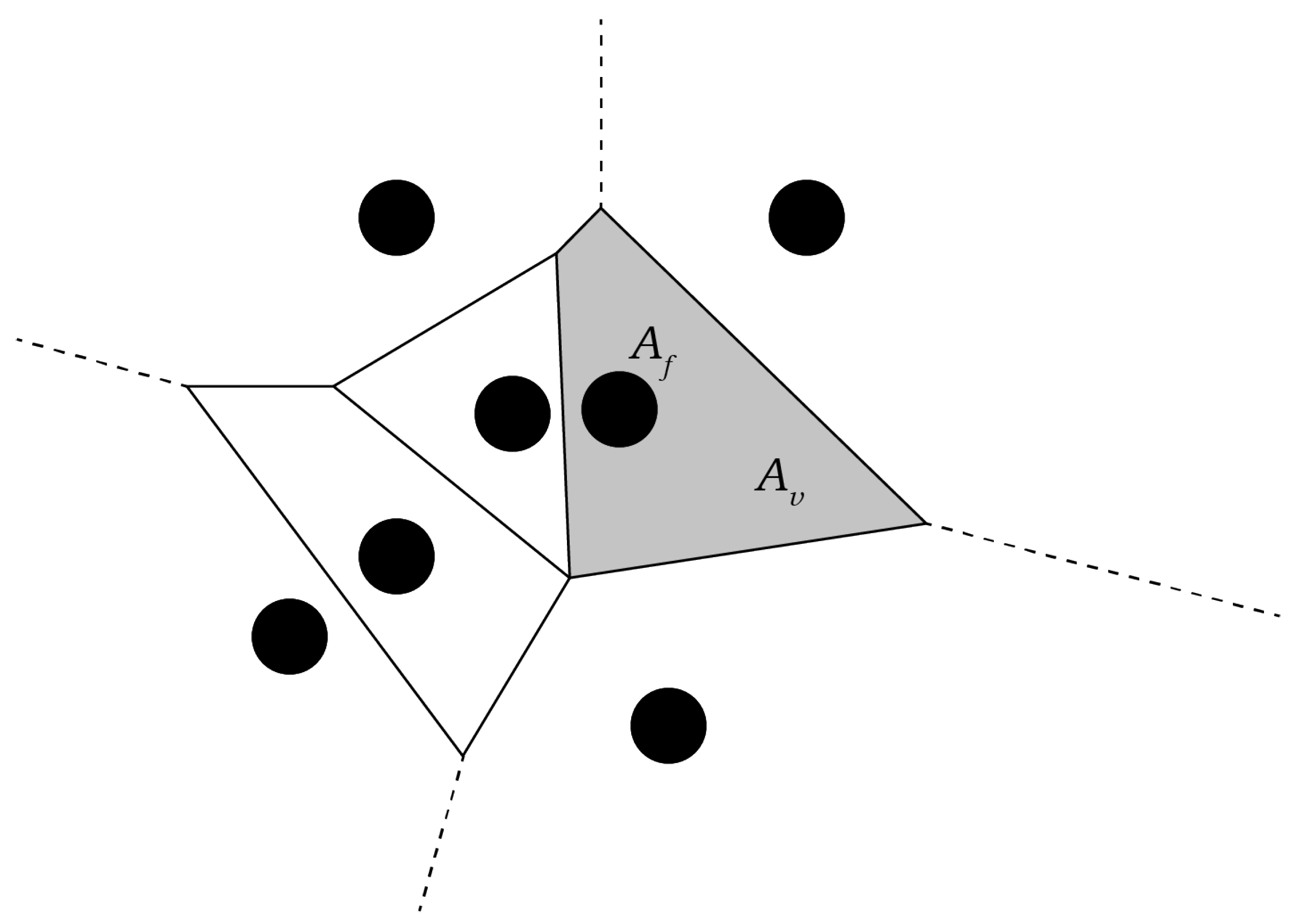
Considering a cross-sectional micrograph of an unidirectional composite, the general approach is to associate a cell of a Voronoi tessellation, also referred to as Dirichlet region [14], to each fibre centre. A Voronoi cell consists of a convex closed polygon, where any polygon location is closer to its fibre centre than any other fibre centre [13]. Assuming a known fibre diameter, respectively, its cross section , and knowing the Voronoi cell area allows assigning a Voronoi-based local fibre volume content (Equation (1)) to every individual fibre. An example is shown in Figure 1. The methodology to characterise the unidirectional tape microstructure is visualised in a flow diagram, see Appendix A Figure A1.
2.1. Image Acquisition
Cross-sectional micrographs were prepared from micrographs of carbon fibres with thermoplastics polyethetherketone (PEEK) and polyetherketoneketone (PEKK) matrices, denoted as A, B and C (manufacturers are known to the authors). The tape samples had thicknesses between 0.14 and 0.23 mm and a width of 10 mm. The samples were embedded in Struers EpoFix slow cure and polished on a Struers Tegramin polishing equipment. The images were captured using a Keyence VK-X1000 3D (Keyence Corporation, Osaka, Japan) laser scanning confocal microscope at 50× magnification in its optical mode with coaxial lighting and using its automated stitching capabilities. The stitched images were saved with the Keyence Multi FileAnalyzer software in its proprietary format and had a resolution of 17,000 × 700 pixels to capture the whole cross-section of the embedded samples.
2.2. Image Analysis
Based on the aforementioned micrographs, the 5 principal steps—fibre centre detection, fibre radius calculation, boundary detection, the Voronoi tessellation with boundary elements, and the top and bottom through surface analyses—are discussed in further detail.
2.2.1. Fibre and Fibre Centre Detection
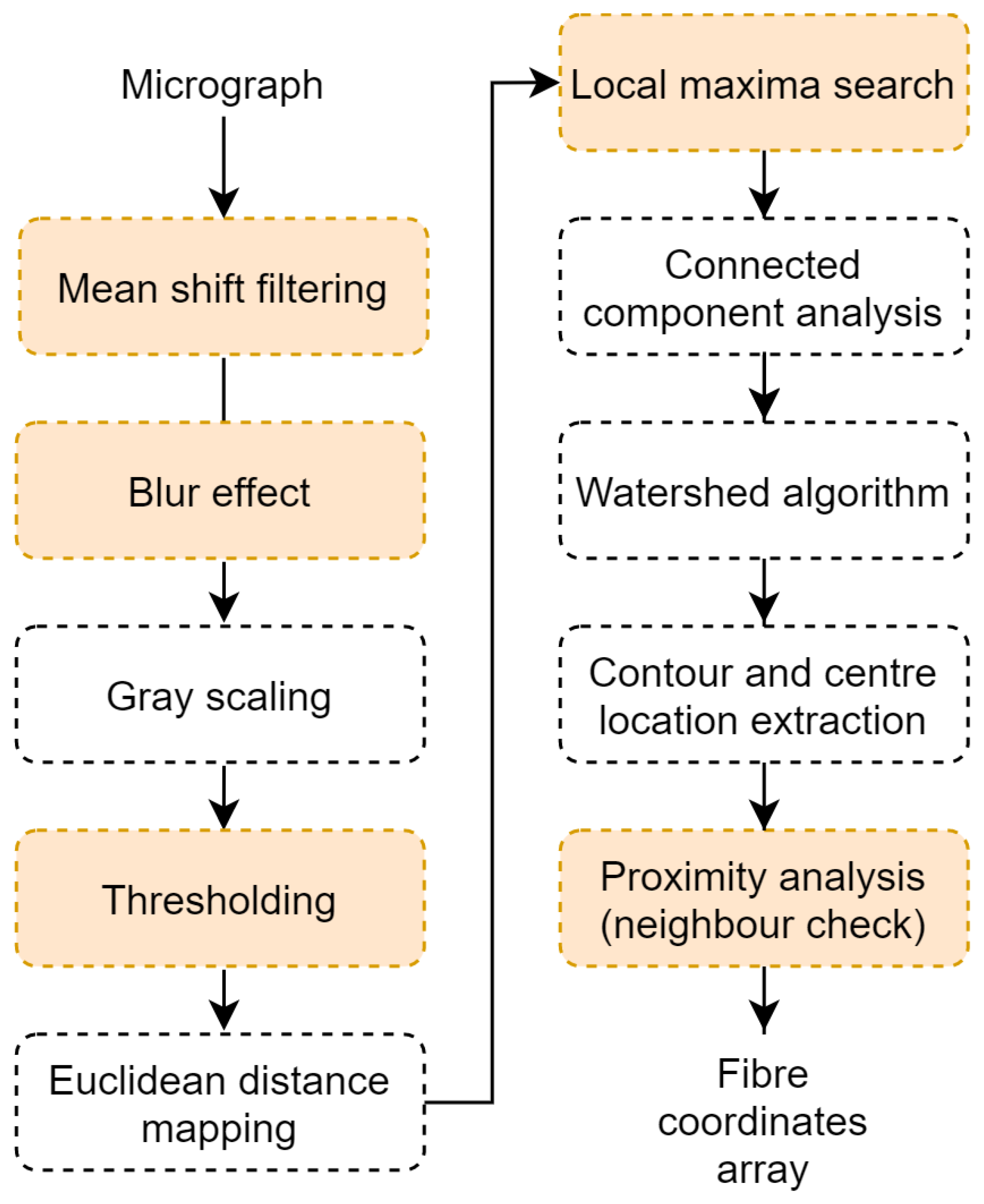
The main steps to detect fibres and corresponding fibre centres are visualised in Figure 2. The Hough circle transform algorithm [12,15] is widely used in image processing and computer vision to detect circular inclusions and its centres. It does, however, require significant computing power and memory for these large datasets. In this work, the Python library OpenCV is used to define the fibre contours based on a watershed of the input micrographs [16].
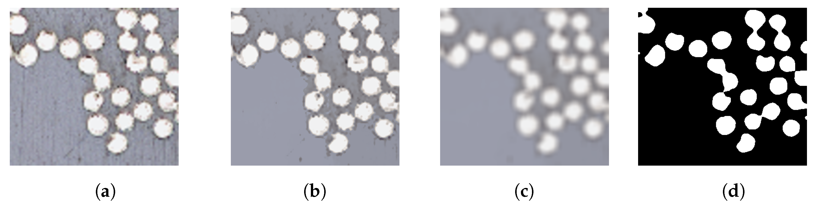
Before applying the watershed algorithm, the image is preprocessed: first, the fibres are separated from the background using mean-shift segmentation (Figure 3b). The pixel intensity of every single pixel is compared with surrounding pixels and modified accordingly if needed based on the parameters spatial window radius (Sr) and the spatial colour radius (Sp) [17]. The mean shift segmentation of a pixel includes neighbouring pixels which are spatially close (Sr) and have a colour intensity within the specified colour radius (Sp).
Subsequently, the image is blurred (Figure 3c) and converted to greyscale. Because the lightning conditions slightly vary over the length of large micrographs, using only global thresholding is not sufficient [12]. An equal weighted square matrix kernel, K is specified and applied to each single pixel to determine which neighbour pixels are used to calculate the mean value for that specific pixel.
Adaptive thresholding in terms of Binary thresholding combined with Otu’s thresholding is applied (Figure 3d). Instead of a constant thresholding value, a dynamic thresholding value is determined using OpenCV which is based on a small pixel region and its corresponding image histogram [18,19].
The binary image is used to create an Euclidean distance mapping matrix. Subsequently, a local maxima search is performed on this matrix to identify the matrix entries with the highest Euclidean distance [18]. The local maxima in this matrix do not directly correspond to the fibre centres: often two or more neighbouring matrix entries are defined as the local maxima for a specific fibre because of an equivalent Euclidean distance. Therefore, the actual fibre centres are determined based on contours which are defined using the local maxima matrix in combination with the original micrograph input.
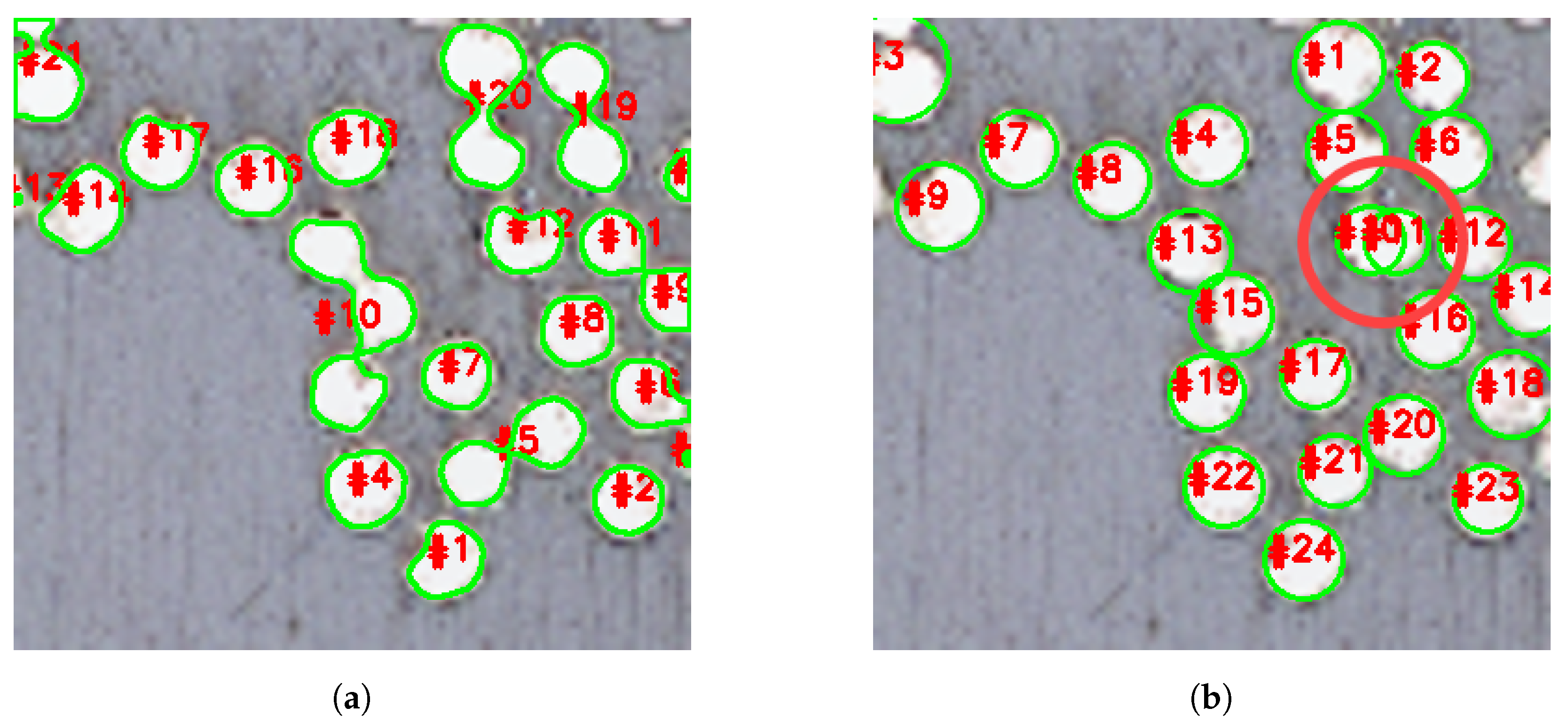
The high packing density of the fibres combined with a level of clustering makes the extraction of individual fibre features from a binary image very challenging, if not impossible. Without the application of any intermediate step, the contours using OpenCV are defined as presented in Figure 4a. Similar to the work in [9] related to composite micrographs, the watershed algorithm is used to distinguish the fibres from the matrix. The necessity of the so-called topological 8-connectivity watershed [20] is clearly visible when considering contour number 10 of Figure 4a and contours 13, 15 and 19 of Figure 4b where each individual fibre is identified by a single contour with corresponding circle radius.
The final step is a proximity analysis of each individual fibre centre location based on the nearest neighbour distance: the fibre centres closer to each other than the specified tape dependent parameter (Minimum fibre diameter) are combined to one unique fibre centre point. This parameter is referred to as in this work. As an example, the fibre centres of contour number 10 and 11 in Figure 4b, marked with the red circle, are merged to one fibre centre.
2.2.2. Fibre Radius Calculation
Initially, the fibre radii were determined based on the defined contours as presented in Figure 4b. It was found that this method does not accurately determines the fibre radii: it was impossible to set the threshold values such that all fibres were captured. Inaccuracies originated because of several reasons: One reason is the presence of shadow regions in the micrographs in the vicinity of the tape boundaries which results in different thresholding behaviour. Besides, slight contrast differences are present within the same micrograph, effecting the result of thresholding. Another reason why this method was found to be inaccurate is the fact that in some cases fibres were damaged, possibly during grinding and polishing, resulting in several fibre pieces scattered in a small region. Heavily thresholding resulted in removal of these small particles, whereas no to little thresholding in combination with the contour algorithm resulted in several defined small regions (i.e., fibres). Because of this rather uncontrollable process of radii definition, a different and more generally applicable method was required. It was found that based on greyscale values of the centre pixels the fibre radius can be determined with increased accuracy.
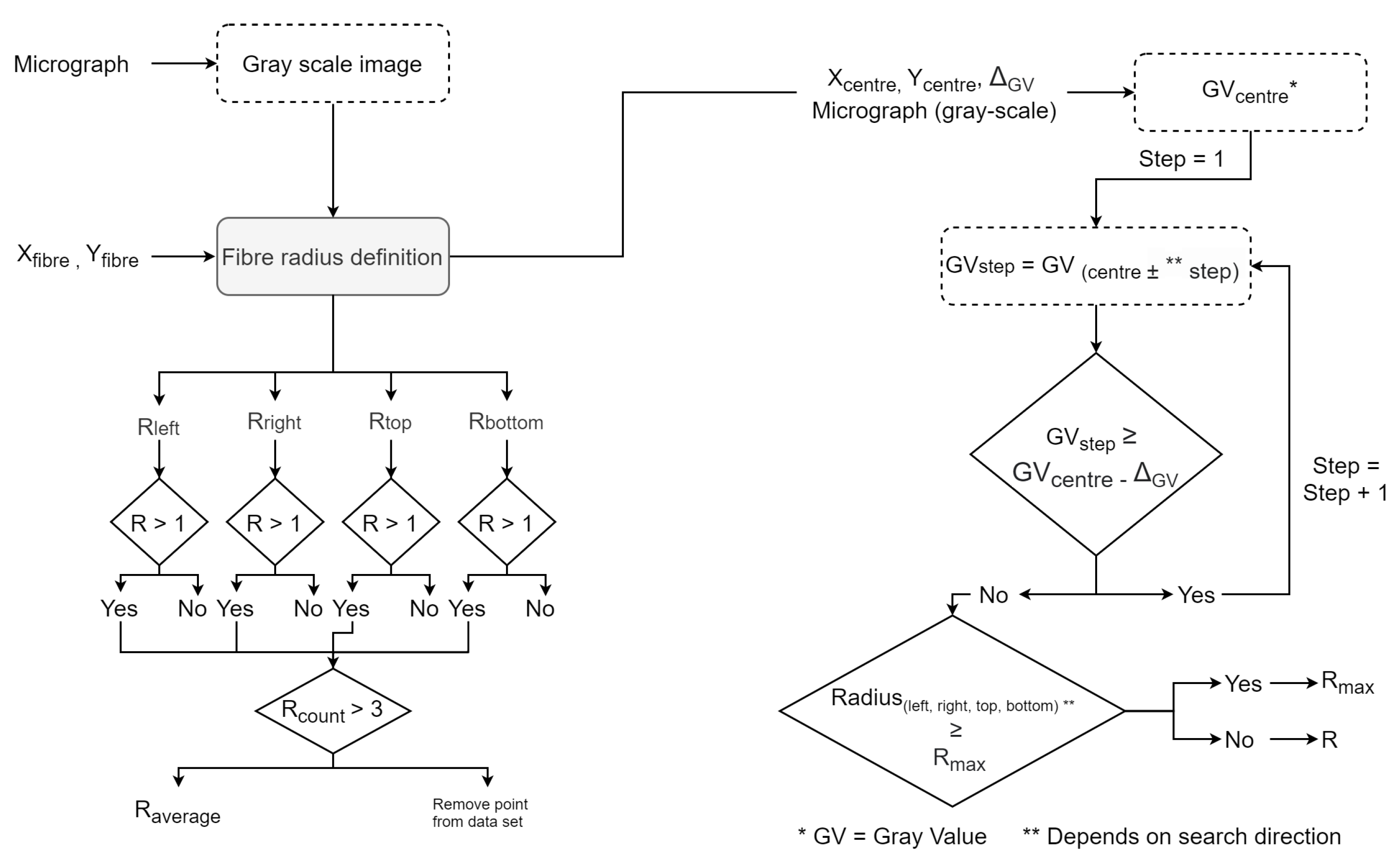
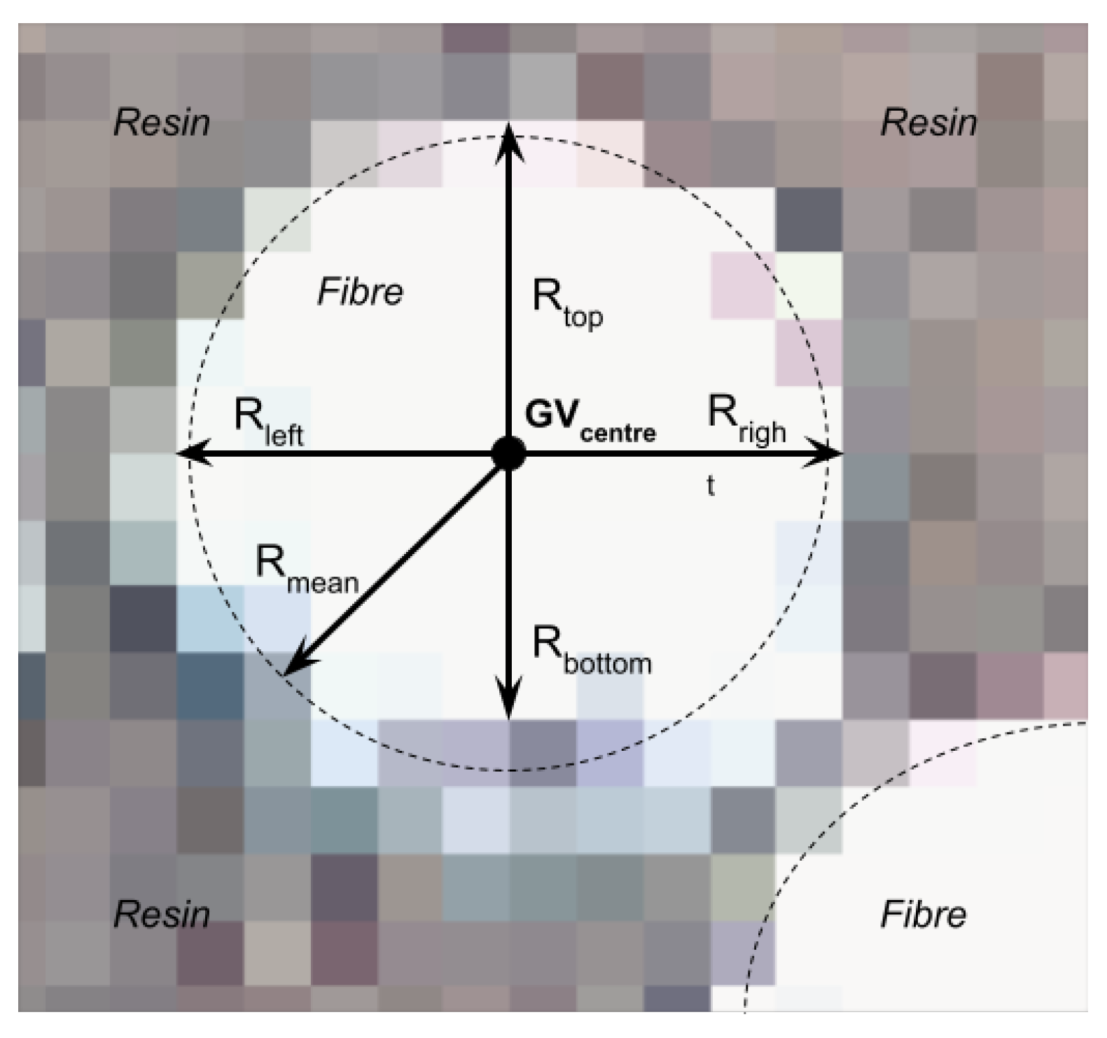
First, the centre points of the defined contours are used as input for this part of the algorithm. False detections of fibre centres outside the defined boundary polygon are neglected a priori. A fibre radius function is used four times to determine the radius in four directions, left, right, top and bottom to eventually determine the average fibre radius (left of Figure 5). The grey-value of the centre pixel is the leading variable in this radius definition function and the grey value offset () determines whether or not a pixel is considered part of the fibre, refer to Figure 6. The offset is subtracted from the greyscale pixel intensity of the centre pixel (right block of Figure 5, meaning that the radius of a fibre in the shaded region of the UD tape can be determined with increased precision. Besides , where the next applicable pixel depends on the direction of search, the found radius R value is compared with a specified . The specified maximum radius is considered in the average radius calculation in case one of the defined radii is larger than this defined maximum value. Besides this check, before calculation of the average fibre radius the defined radii are tested to a criteria specifying a minimum amount of three radii having a value of at least one pixel. Eventually the average fibre radius is compared with a specified minimum fibre radius. If either one of both tests fail, the detected fibre is considered an erroneous detection and it is removed from the data set. The aforementioned two criteria deal with the ambiguous detection of clustered fibre particles. Both and can be determined by iteratively overlaying circles on the fibres in the micrograph with corresponding (defined) radii.
2.2.3. Boundary Detection
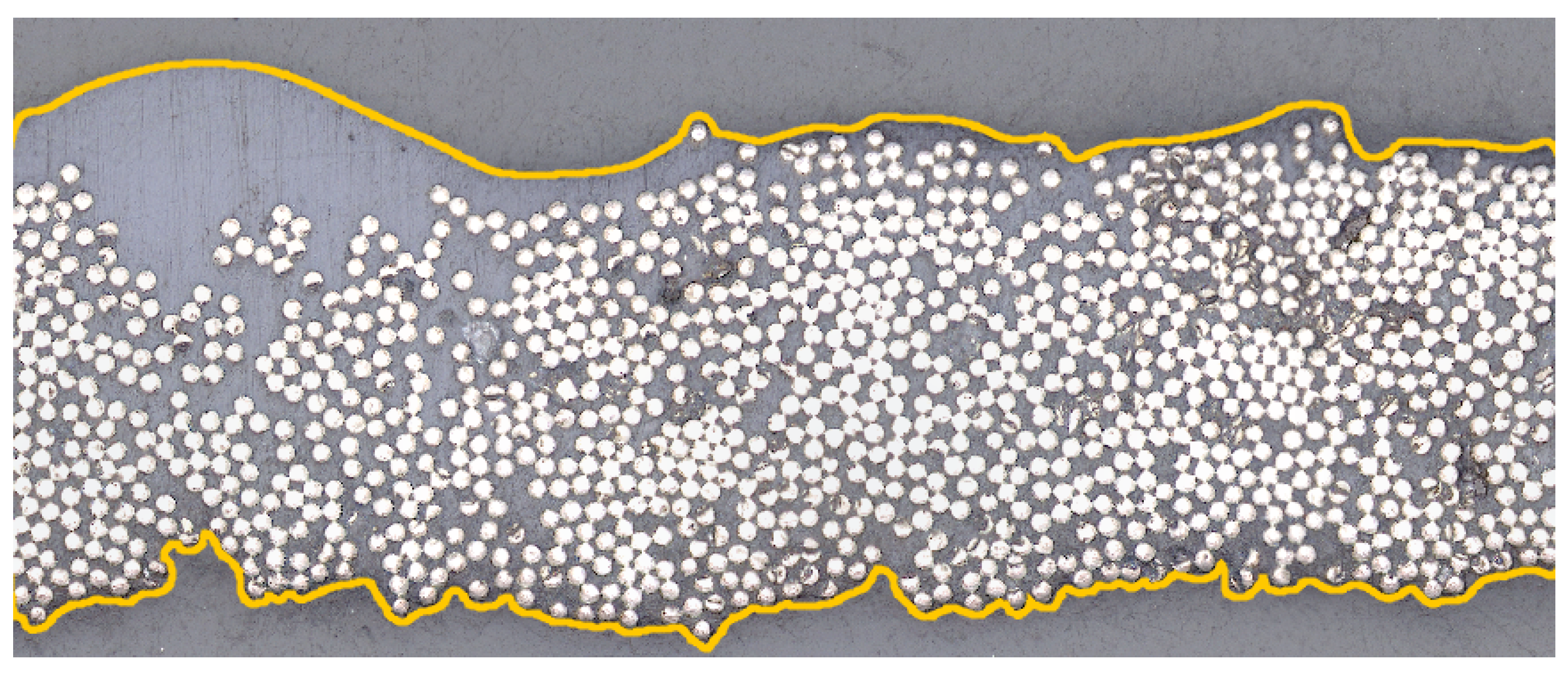
In standard Voronoi tessellation, the outermost centre points lead to infinite size Voronoi elements and can therefore not be included in the analysis. However, the local fibre volume content at the tape surface is of interest. Here, a manual interactive method of defining the boundary as a polygon in ImageJ is used using the ‘Polygon selection’ option in ImageJ as shown in Figure 7. To increase the manual boundary definition, three additional points are added between each defined point by using interpolation. Depending on boundary contrast or imaging technique, the boundary detection could also be automatised in the future via image processing. Combining the tape boundary polygon with the infinite Voronoi tessellation yields in artificial finite boundary points, schematically visualised in Figure 8.
2.2.4. Voronoi Tessellation with Boundary Elements
With the fibre’s vertices known, using the Voronoi function of SciPy, a Voronoi tessellation is created with the vertices of the outermost cell vertices having an infinite value. These points were consecutively moved to the intersection of the polymer matrix boundary polygon created in Section 2.2.3. More details can be found in the algorithm sub-function voronoi_finite_polygons_2d of the Python code of the digital appendix.
2.2.5. Top or Bottom Surface and through Thickness Analyses
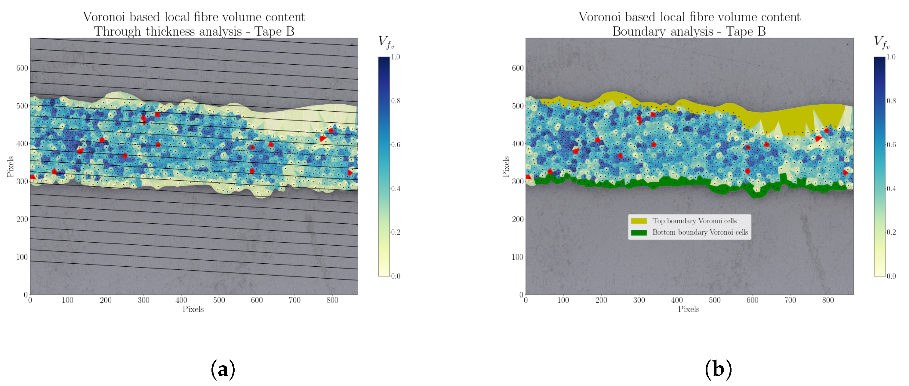
With the complete Voronoi tessellation, identified fibre radii and identified surface elements, additional analyses can be carried out such as surface analyses by selecting only the top or bottom surface Voronoi cells for individual analyses. To evaluate through thickness distributions, the tape micrograph was discretised into 10 parallel equidistant slices which were evaluated for through thickness analyses. The fibres, including corresponding Voronoi cells, within a thickness slice make up the mean value for that specific thickness segment. A typical result for a B type tape is shown in Figure 9a. The Voronoi cells marked in red have a larger than one, i.e., the fibre area is defined larger than the area of the corresponding Voronoi cell.
3. Application
3.1. Comparison of Unidirectional Tape Manufacturing Methods
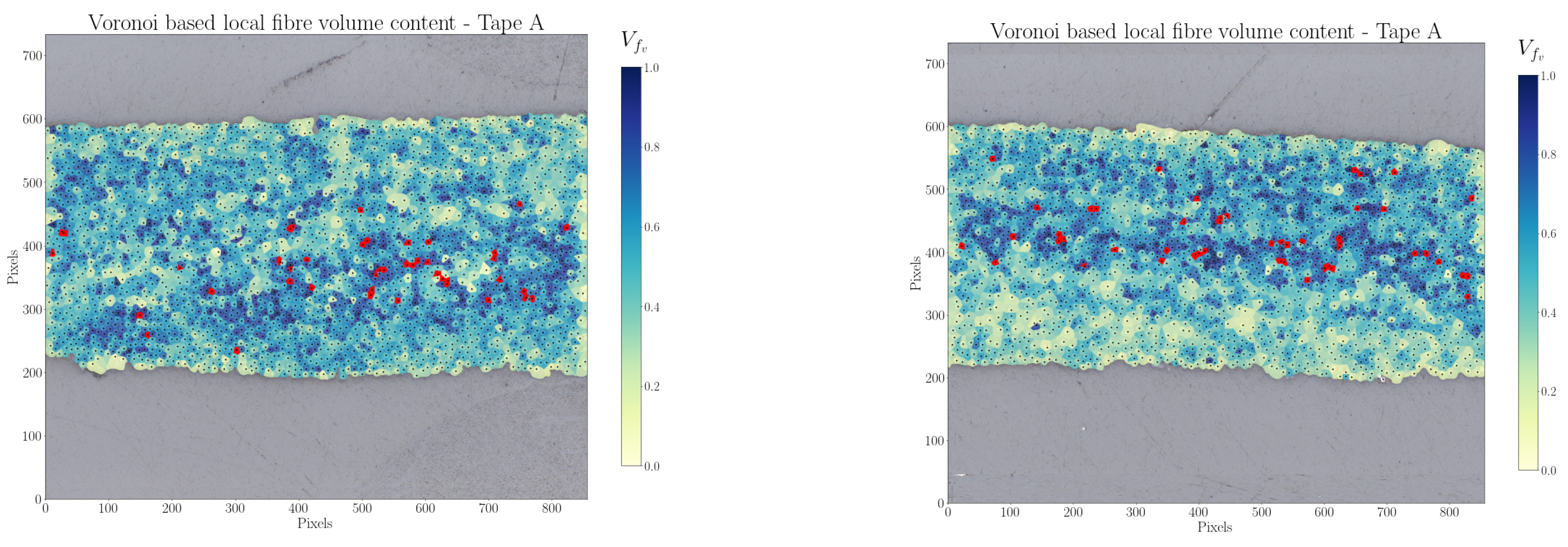
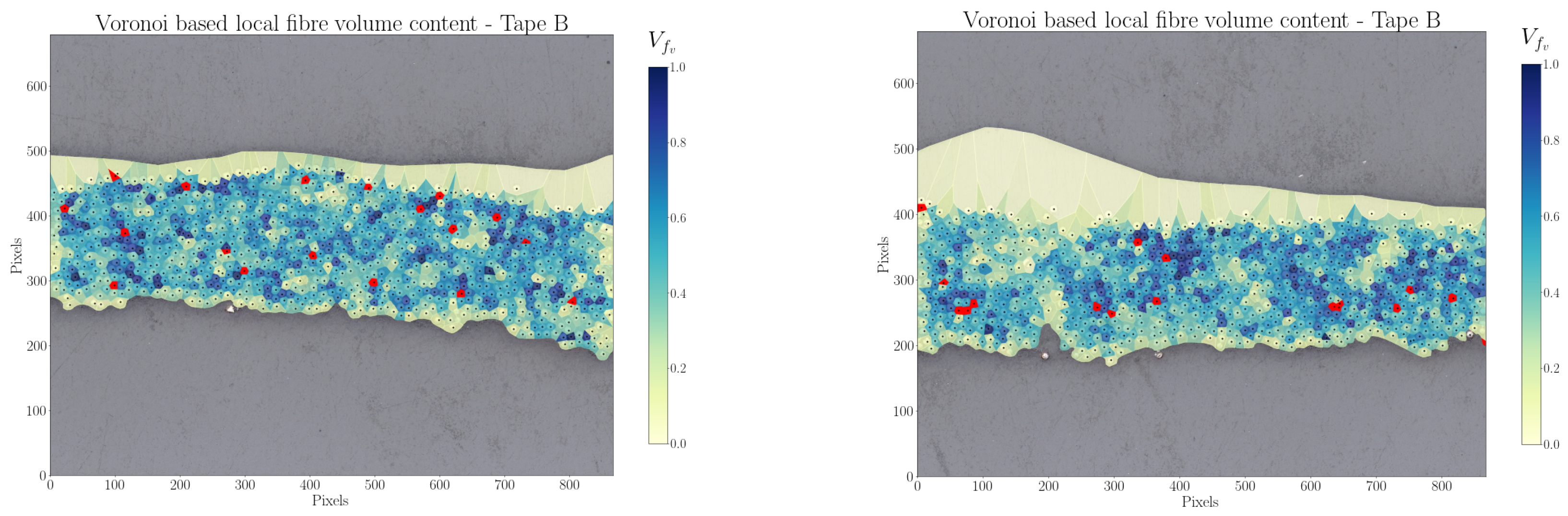
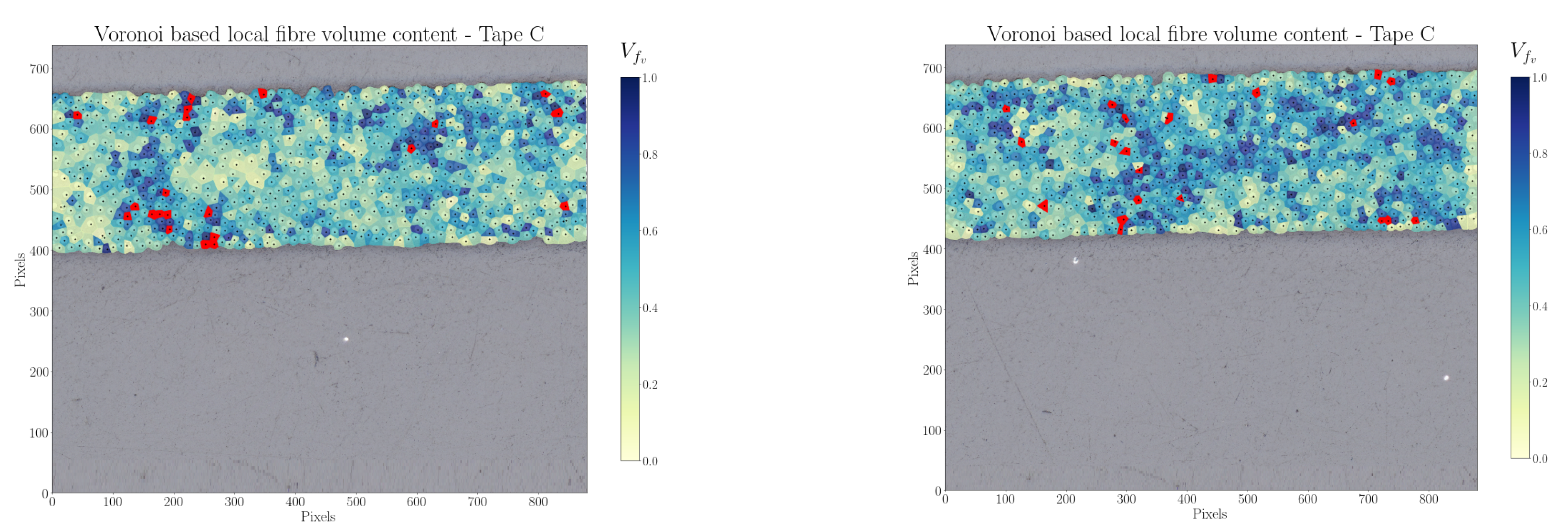
To demonstrate the method in an application context, three unidirectional tapes, denoted A, B and C (manufacturers are known to the authors), originating from different impregnation methods [21,22] have been investigated. To capture the variability of the respective product, two neighbouring micrographs have been generated from each material to better capture mesoscopic variations (see Figure 10, Figure 11 and Figure 12).
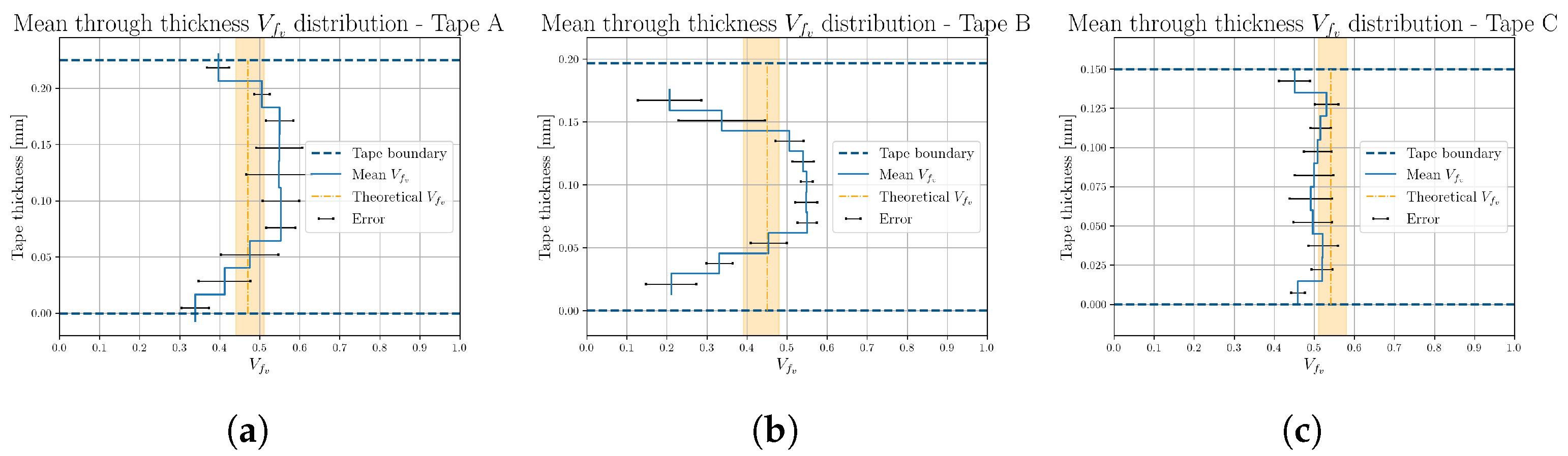
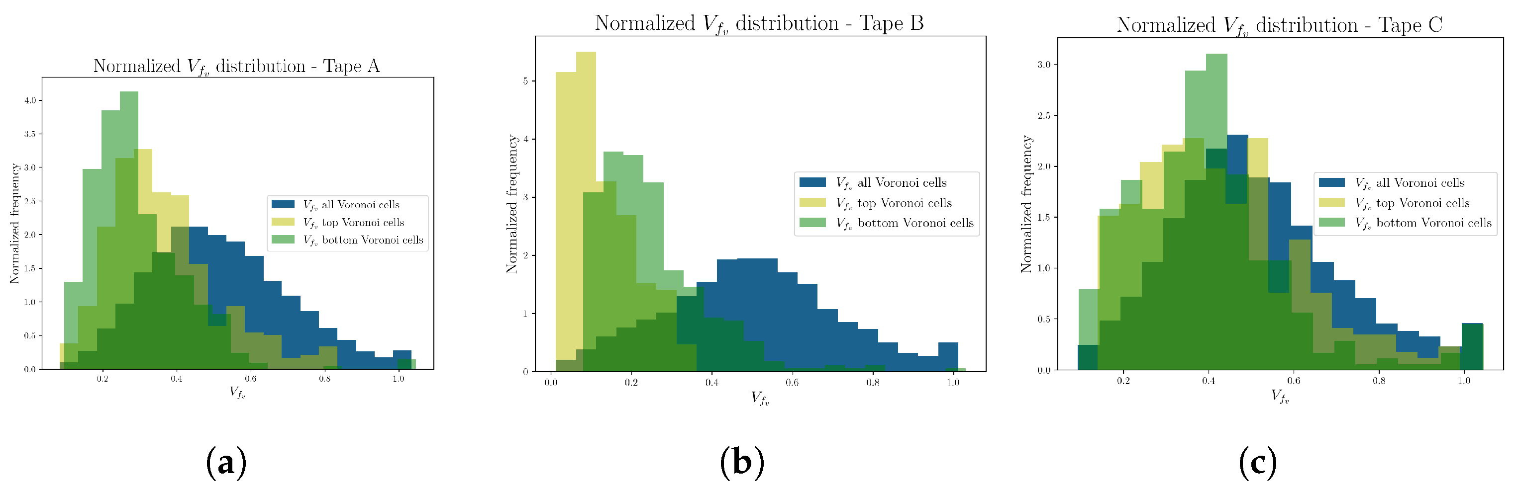
Large variations in homogeneity of fibre volume content were observed in the tapes A and B. Tape C shows minor variations but still no perfectly homogeneous distribution of fibres, which is rarely found in real microstructures [11]. Tape A seems to have a resin rich surface showing layered mesoscopic fluctuations in fibre content. Tape B shows distinct resin rich area on the top side, while tape C appears the most homogeneous. These observations are confirmed in the through thickness analysis of Figure 13, where the mean fibre volume is shown as a function of the thickness. The theoretical fibre volume fraction is presented as a single value using an orange dotted line. This value is based on the mean tape thickness of the samples. The tape samples used showed minor thickness variations, which leads to a bandwidth of theoretical values. Variations in per thickness segment, i.e., the error bars, could be established as multiple micrograph sections were analysed for tape A, B and C. The variations through the thickness is in line with other descriptors also varying through the thickness in other work by this research group [23].
Individually selecting the Voronoi cells of the top and bottom layer allowed further elucidation of surface features. Figure 14 reveals distinct contrasting surface features for tape A and B, in particular the top surface of tape be having a local below 10 percent. The analysis also confirms the rather homogeneous distribution of of tape C, with surface values only slightly deviating from the bulk values.
Summarising, this microstructural analysis method of cross-sectional micrographs, can be used to discriminate characteristic features of unidirectional tapes originating from different manufacturing routes [21,22]. The inclusion of the surface boundary permits a dedicated analysis of the Voronoi cell attributes to the outermost fibre layer, which reveals specific surface features of high relevance to processability, the creation of intimate contact and reptation, such as in laser assisted tape laying [6], compression moulding or open mould autoclave processes.
3.2. Sensitivity Analysis
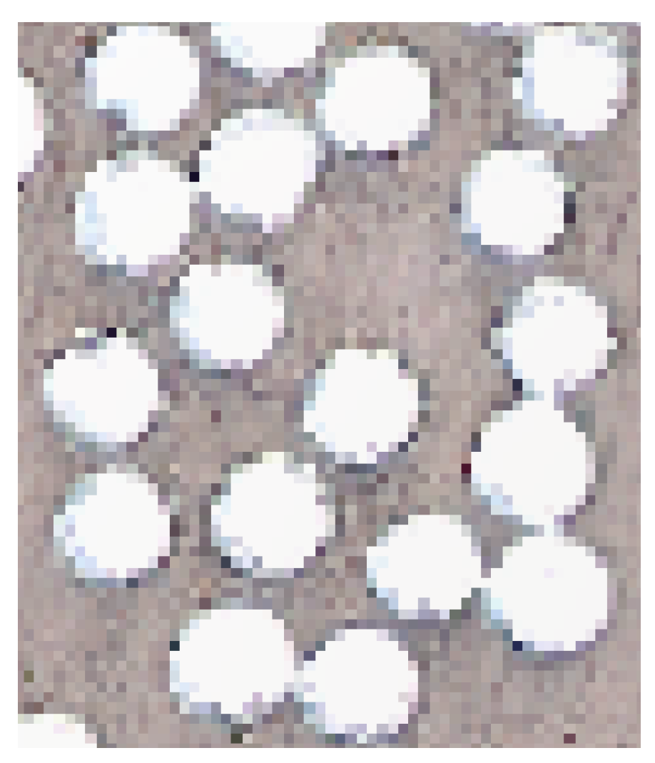
To address the robustness of the methods described so far, a representative section of tape C is used to investigate the sensitivity of the methods. The modifiable parameters involved are separated in two groups: the first group of parameters is related to fibre detection and fibre centres determination (Sr, Sp, K and ), and the other group are the fibre radii determination related parameters ( and ). Subsequently, their effects are tested on a representative micrograph section, shown in Figure 15.
3.2.1. Fibre Detection and Fibre Centre Definition Parameter Sensitivity
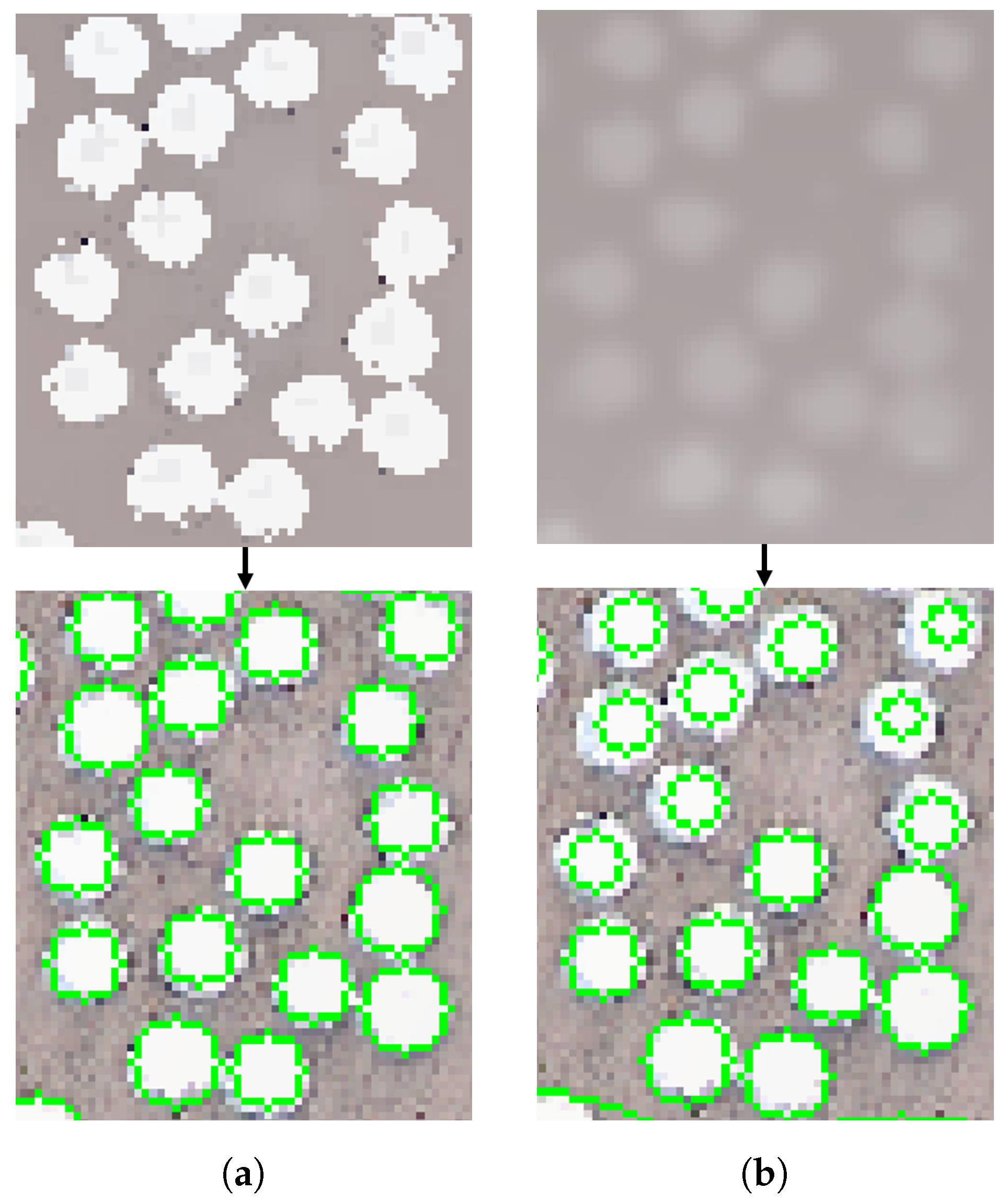
Mean shift filtering is applied to the original micrograph to increase edge detection of the fibres. This algorithm is based on two parameters: the spatial window radius Sp and the spatial colour radius Sr [19]. To check the sensitivity of the obtained fibre and fibre centre, in Figure 16 both the optimal values (Figure 16a) and extreme values (Figure 16b) are used. As can be visually observed, the extreme values lead to a figure where the fibres are not as clearly distinguishable. However, based on the defined contours, shown on the bottom of the figure, this function is stable with respect to variations in both input parameters Sp and Sr. Since only the centre of the defined contour is used in the overall algorithm, small shifts of fibre centre do not result in large differences in the mean fibre radius value (see Section 2.2.2). However, for large shifts the four determined radii cannot be considered accurate any more. The latter because of the contours being assumed to be circular.
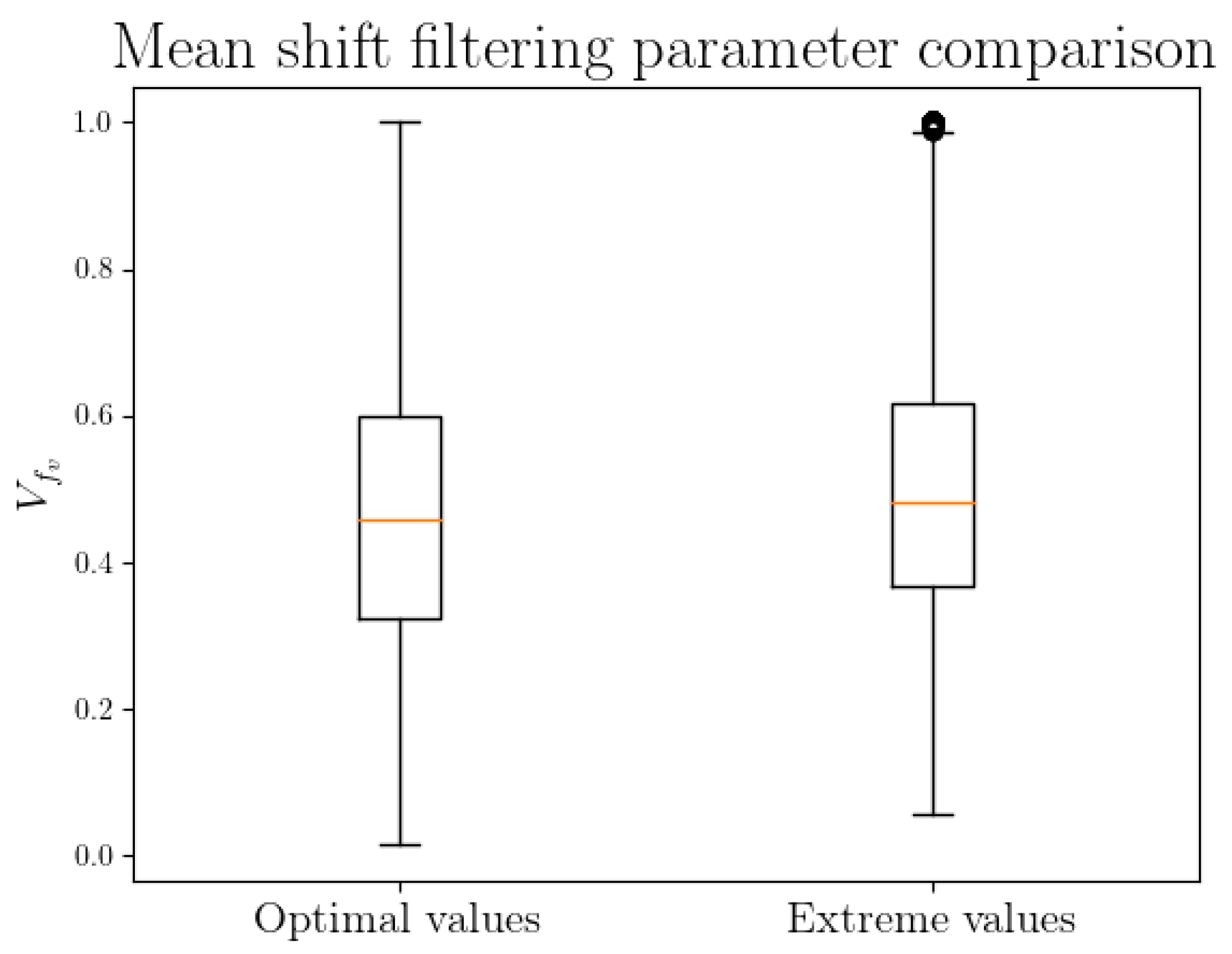
As the Voronoi based local fibre volume content depends on the fibre cross section and hence the fibre radius, the stability of the fibre centre and fibre radius computation can be validated by determining the for several micrographs using the two aforementioned parameters, Sp and Sr (Figure 17). It could be observed that there is little difference in for optimal or extreme mean shift filtering settings.
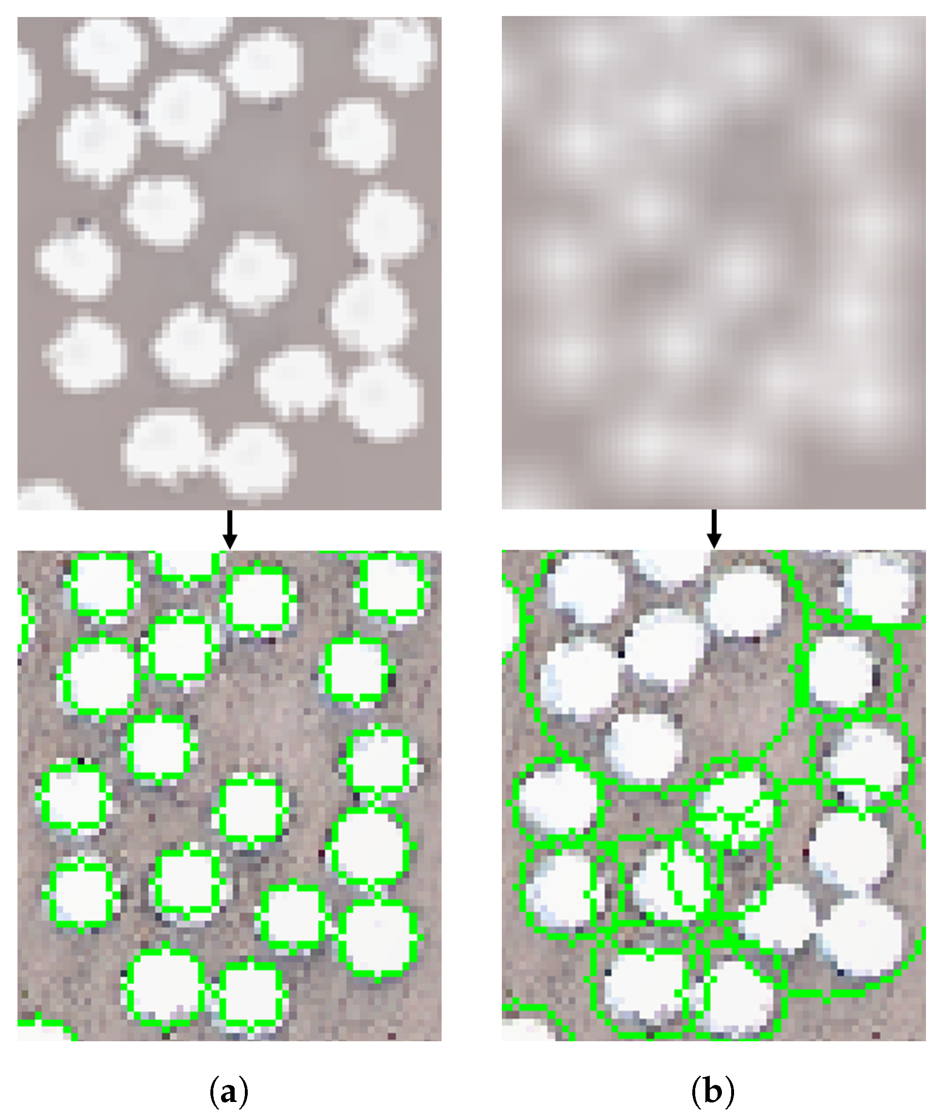
Subsequently the blur effect is used to average the pixel intensity of each individual pixel. The openCV blur function is based on a square matrix kernel [19]. A larger kernel results in averaging the pixel intensity based on more surrounding pixels, visualised in the top part of Figure 18. It can be seen that applying a larger blur kernel results in only the fibre centres being slightly visible. Based on the drawn green contours presented in the lower part of Figure 18, it can be concluded that the size of the kernel has a significant influence on how accurate the fibre contours are defined. A few contours are relatively well defined: their centres are still on, or close to, the actual fibre centre. However, some contours are not defining any fibre whereas other contours are drawn around multiple fibres. This result emphasises that the micrographs are sensitive to the blur setting chosen. A kernel too large clearly disturbs the contour definition of the fibres.
To obtain a binary image, thresholding is applied to the blurred micrograph image. As Zangenberg et al. mentioned, single value thresholding (i.e., global thresholding) is sufficient once the lighting conditions over the micrograph do not vary. The relatively large micrograph sections used in this work require adaptive thresholding for an optimal result. This implies that different thresholds are used for different parts of the micrograph. These varying thresholds are based on the image histogram of that particular section. Otsu’s thresholding technique was found to be the most suitable for this application [19,24]. As Otsu’s algorithm from OpenCV automatically determines the thresholding values, this image processing step is stable and can be repeated with the same results.
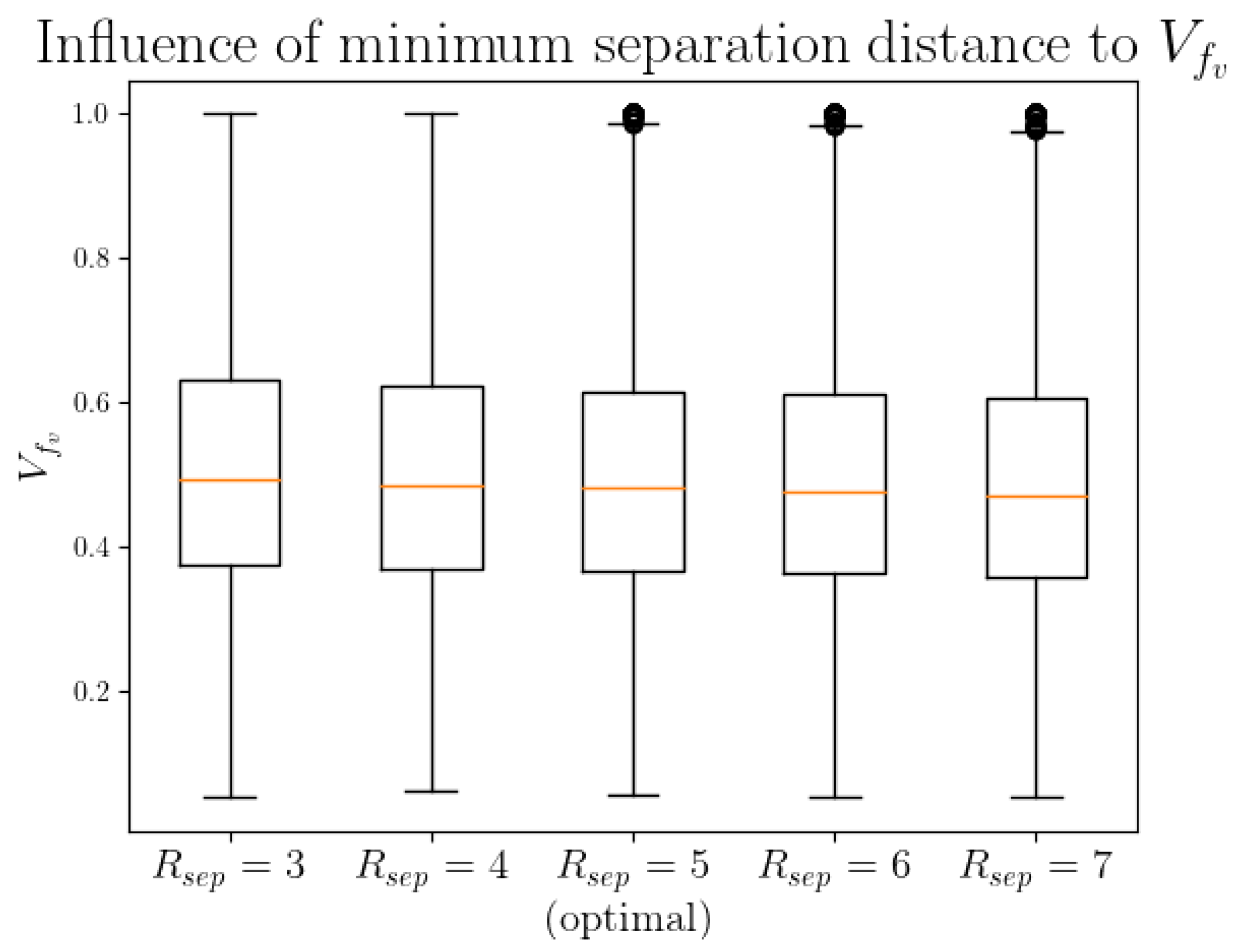
The Euclidean distance map and the proximity analysis (shown in Figure 2) both use a defined parameter specifying the minimum theoretical distance between two fibres, . This parameter is already used before (Euclidean distance mapping) and after (proximity analysis) the fibre contours are defined. The optimal value is the mean fibre radius, which can be measured in the original micrograph and should roughly correspond to the mean fibre diameter from the composite material product data sheet. Figure 19 shows that a variation of the mean radius has little to no influence to the final distribution. This can be explained by the fact that the fibres in the unidirectional tapes analysed are not (always) in contact with each other.
3.2.2. Fibre Radii Calculation Parameter Sensitivity
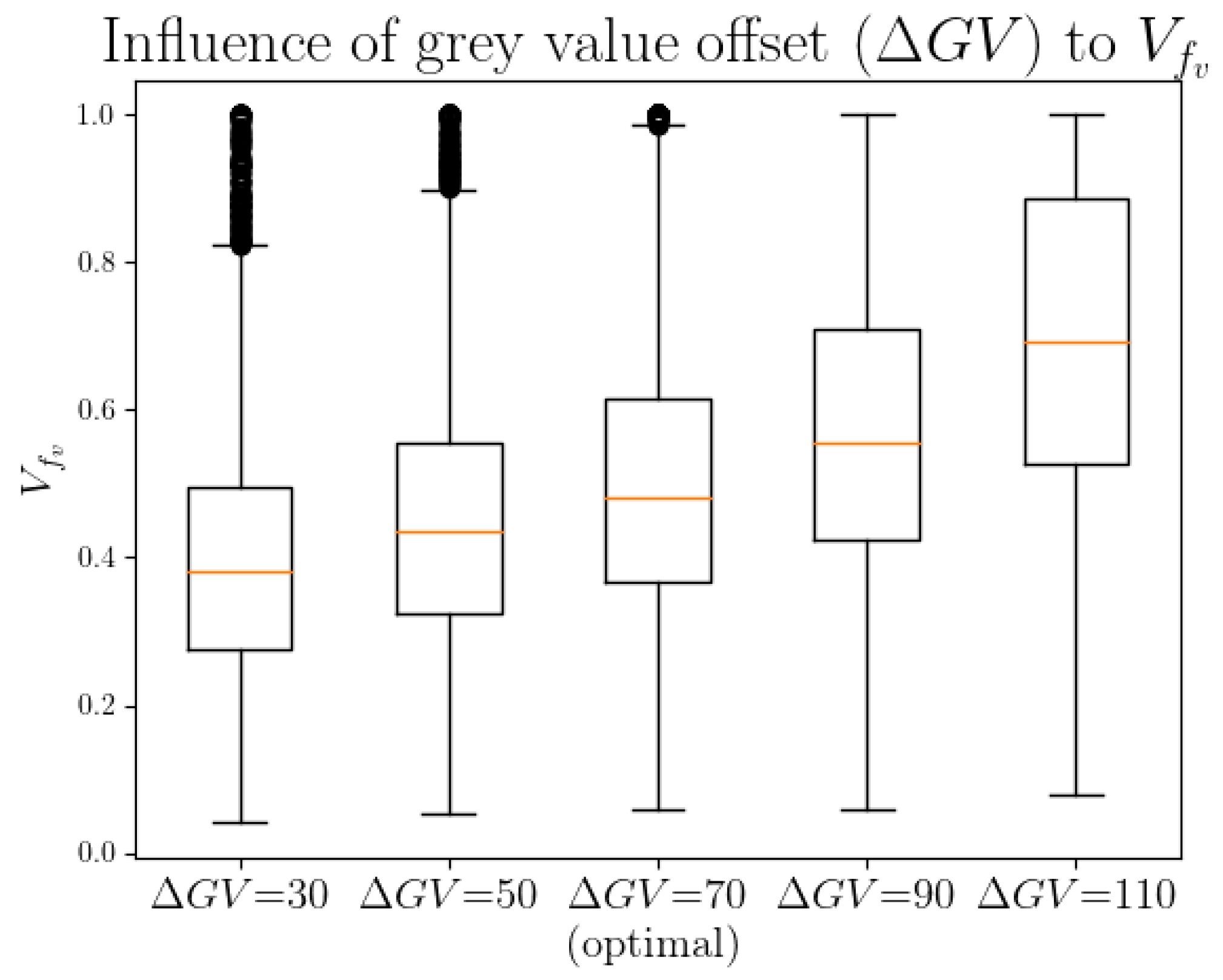
The first parameter involved in the fibre radius calculation which is tested on its sensitivity is the grey value offset (). In the iterative radii search, a pixel is considered part of the fibre if its intensity is larger than the intensity of the centre pixel minus the grey value offset . In other words, a too large results in over predicting of the fibre radius, and vice versa.
The variations in chosen are large: while the optimal is 70, the values 30, 50, 90 and 110 are also tested. The results are as expected: when reducing to 50, the obtained volume fraction remains almost the same, but slightly lower compared to the optimal value which is shown in Figure 20. The same holds for a higher of 90: a slightly higher volume fraction is obtained, but the difference is not significant yet. This result indicates that small parts of the fibre are misidentified as resin ( = 50), or the other way around ( = 90). When picking equal to 30 or 110, a significant change in fibre volume fraction can be seen. Given that these values differ by more than 50% compared to the optimal value, the sensitivity of the is deemed to be low.
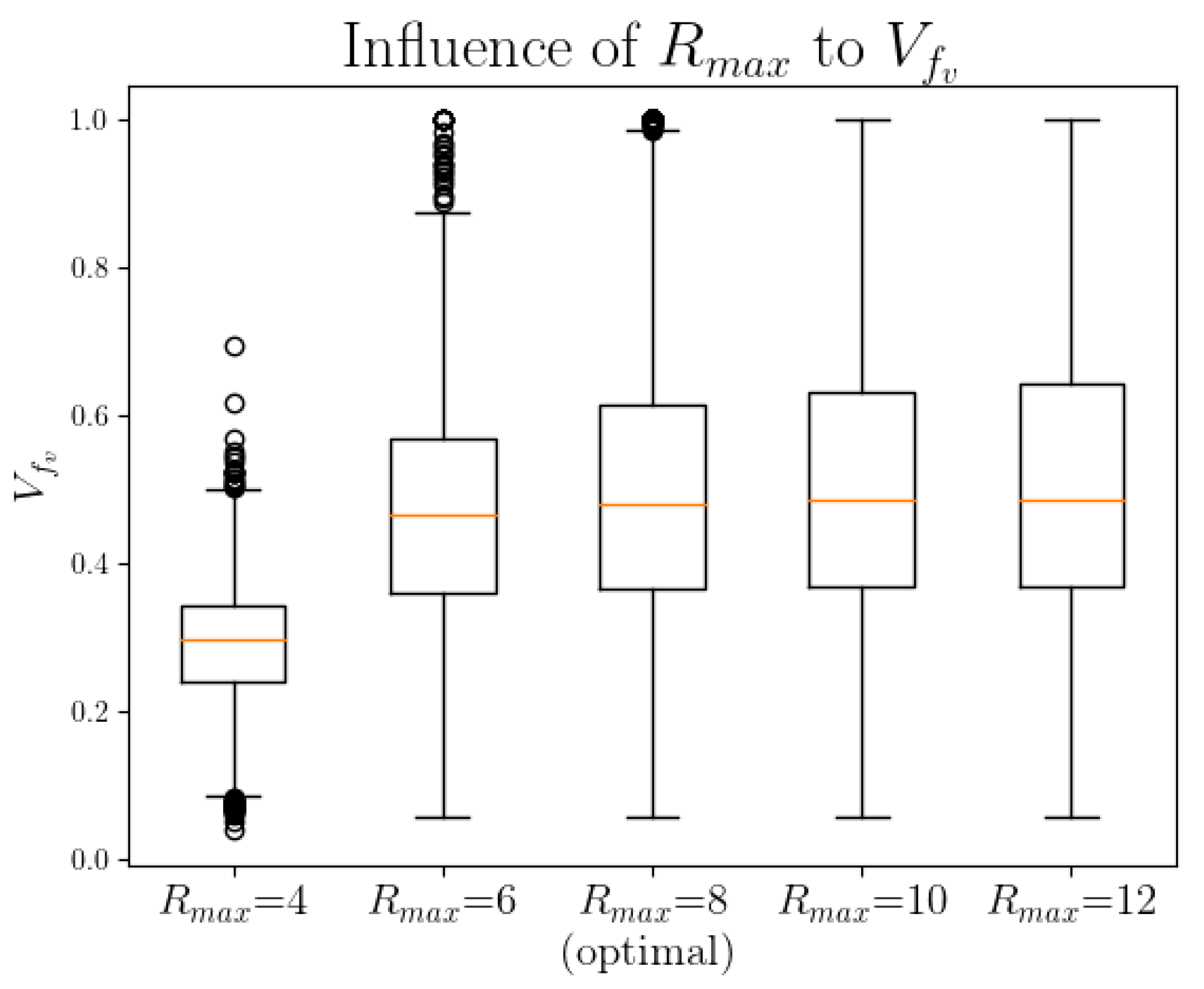
The last tunable parameter is the predefined maximum fibre radius, . This parameter was introduced as it was observed occasionally that the iterative radii search starting at a specific fibre centre jumped over to an adjacent fibre. This is prevented by specifying a maximum radius. The optimal maximum radius can be defined by analysing the original micrographs. With the possibility of detection of larger fibres, can also increase, see Figure 21. Although a slight increase of is observed, this increase is relatively low in comparison to the variation in . With the current algorithm, the change in results is negligible if the value is specified one or two pixels away from the optimal .
4. Discussion
This paper showed that distinct microstructural features in the cross-sectional analysis of unidirectional composites can be identified with the method described. The through-thickness variation and overall homogeneity of the different tapes showed distinct behaviour between the tapes in terms of homogeneity. This information is important when building RVEs and can have a significant influence on the stress distribution throughout the thickness of the tape in the final product. Furthermore, the amount of fibres and resin close at the surface was shown to be different, having implications to future processing, for example, in the case of laser-assisted fibre placement where resin at the edge was shown to be a key feature [6].
Experience has shown that with good quality micrographs the method is robust and has the potential to be automated. While the outer boundary was digitised manually here, an automatic boundary detection is possible, provided a sufficient contrast can be established. This contrast can be achieved for example by the choice of embedding resin in case of an optical micrograph.
The fibre centre and fibre radius detection with 8-connectivity watershed proved robust in spite of the pixel resolution corresponding to only about 1/10th of the fibre radius. The robustness was shown by varying some key parameters, showing that the result almost stayed the same. The method also seems computationally efficient compared to the Hough transform technique [25], known for its computational complexity.
The sensitivity analysis of processing parameters revealed a robust behaviour in respect to the minimum separation distance or maximum fibre radius, respectively, makes it easy to identify optimal settings. The grey value offset does however need attention as it affects the radius detection and it needs to be gauged for a given imaging setup.
With the emergence of high resolution 3D imaging technique such as micro computed tomography [26] this method might also gain relevance for the efficient computation segmentation and reconstruction of fibre slices originated from 3D stacks, contributing to efficient methods of fibre path and fibre diameter reconstruction [27].
Analysing changes in microstructure in composites processing will help to elucidate phenomena such as compaction percolation squeeze flow and its effect in mechanical performance.
5. Conclusions
The microstructure of unidirectional composites is affected by its processing history and influences its structural performance. The method presented allows efficient characterisation of microstructural features through Voronoi tessellation based evaluation of the fibre volume content on cross-sectional micrographs, considering the matrix boundary. The method is shown to be robust and has the potential to be automated. In the future, it could contribute to improved analysis of unidirectional composites in 3D imaging methods to predict their behaviour during subsequent processing.
Author Contributions
N.K. and C.A.D. conceived the investigation and developed the methodology N.K. carried out the analysis and wrote the original manuscript, D.M.J.P. and C.A.D. reviewed and edited the manuscript, C.A.D. supervised the project. All authors have read and agreed to the published version of the manuscript.
Funding
This research received no external funding.
Institutional Review Board Statement
Not applicable.
Informed Consent Statement
Not applicable.
Data Availability Statement
The Python algorithm code used for this work can be downloaded from the following Zenodo-GitHub repository: https://zenodo.org/badge/latestdoi/403121015, accessed on 20 September 2021.
Acknowledgments
Part of the research relates to the master thesis project of N.K. with Boikon B.V. (Leek, The Netherlands). The authors would like to thank Boikon for this opportunity and for providing the UD tape samples.
Conflicts of Interest
The authors declare no conflict of interest.
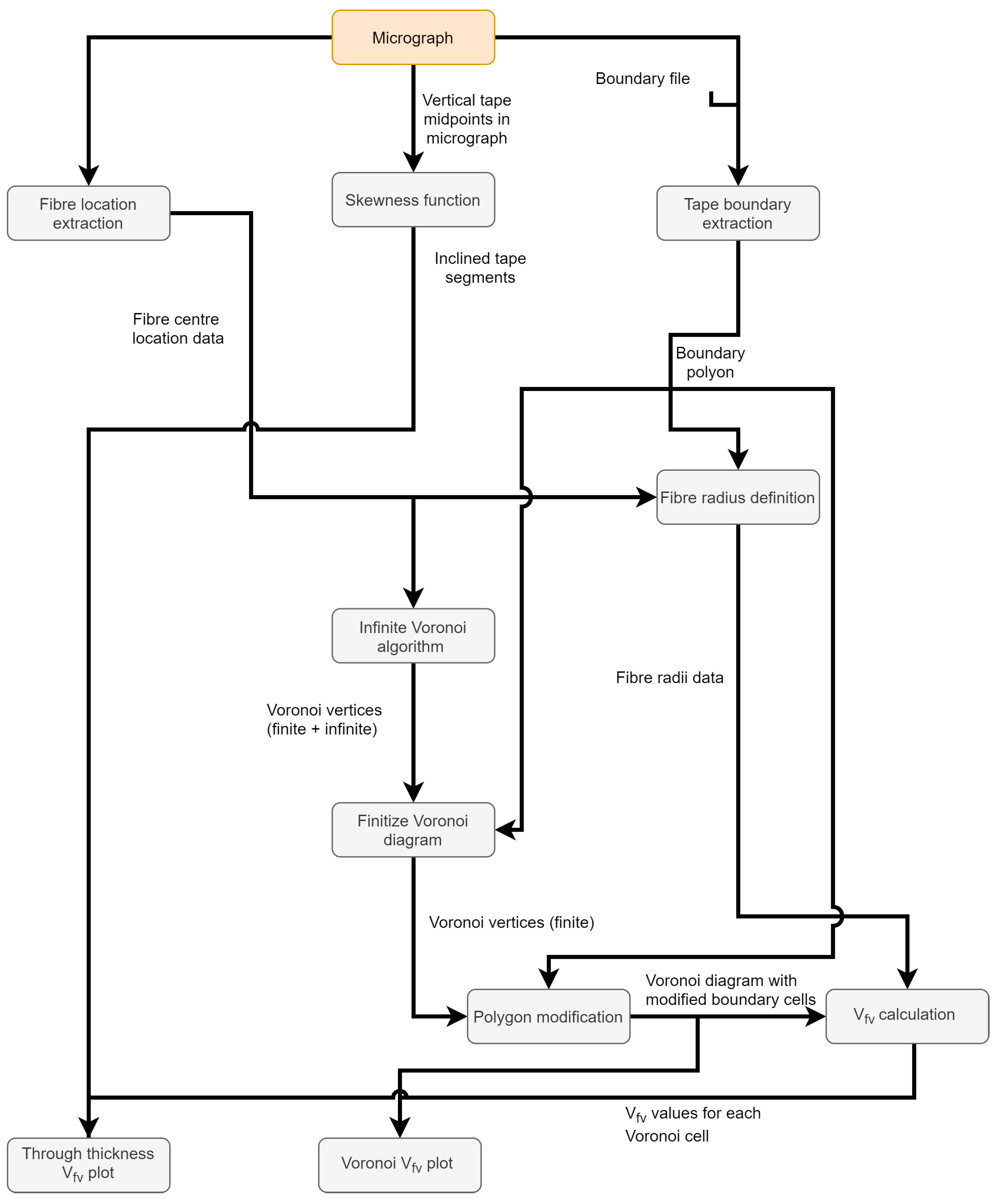
Appendix A. Microstructural Characterisation of Unidirectional Tapes Algorithm Flow Diagram
Figure A1.
Microstructural characterisation algorithm flow diagram.

References
- Schürmann, H. Konstruieren mit Faser-Kunststoff-Verbunden, 2nd ed.; Springer: Berlin/Heidelberg, Germany, 2005. [Google Scholar]
- Meier, U. Carbon fiber reinforced polymer cables: Why? Why not? What if? Arab. J. Sci. Eng. 2012, 37, 399–411. [Google Scholar] [CrossRef] [Green Version]
- Amacher, R.; Cugnoni, J.; Botsis, J.; Sorensen, L.; Smith, W.; Dransfeld, C. Thin ply composites: Experimental characterization and modeling of size-effects. Compos. Sci. Technol. 2014, 101, 121–132. [Google Scholar] [CrossRef]
- Shuler, S.; Advani, S. Transverse squeeze flow of concentrated aligned fibers in viscous fluids. J. Non-Newton. Fluid Mech. 1996, 65, 47–74. [Google Scholar] [CrossRef]
- Slange, T.; Warnet, L.; Grouve, W.; Akkerman, R. Deconsolidation of C/PEEK blanks: On the role of prepreg, blank manufacturing method and conditioning. Compos. Part A Appl. Sci. Manuf. 2018, 113, 189–199. [Google Scholar] [CrossRef] [Green Version]
- Çelik, O.; Peeters, D.; Dransfeld, C.; Teuwen, J. Intimate contact development during laser assisted fiber placement: Microstructure and effect of process parameters. Compos. Part A Appl. Sci. Manuf. 2020, 134, 105888. [Google Scholar] [CrossRef]
- Bargmann, S.; Klusemann, B.; Markmann, J.; Schnabel, J.E.; Schneider, K.; Soyarslan, C.; Wilmers, J. Generation of 3D representative volume elements for heterogeneous materials: A review. Prog. Mater. Sci. 2018, 96, 322–384. [Google Scholar] [CrossRef]
- Vaughan, T.; McCarthy, C. Micromechanical modelling of the transverse damage behaviour in fibre reinforced composites. Compos. Sci. Technol. 2011, 71, 388–396. [Google Scholar] [CrossRef]
- Jeong, G.; Lim, J.; Choi, C.; Kim, S. A virtual experimental approach to evaluate transverse damage behavior of a unidirectional composite considering noncircular fiber cross-sections. Compos. Struct. 2019, 228, 111369. [Google Scholar] [CrossRef]
- Catalanotti, G.; Sebaey, T. An algorithm for the generation of three-dimensional statistically Representative Volume Elements of unidirectional fibre-reinforced plastics: Focusing on the fibres waviness. Compos. Struct. 2019, 227, 111272. [Google Scholar] [CrossRef]
- Schledjewski, R.; Schlarb, A. In-situ consolidation of thermoplastic tape material effects of tape quality on resulting part properties. In Proceedings of the SAMPE Conference, Baltimore, MD, USA, 3–7 June 2007; pp. 3–7. [Google Scholar]
- Zangenberg, J.; Larsen, J.B.; Østergaard, R.C.; Brøndsted, P. Methodology for characterisation of glass fibre composite architecture. Plast. Rubber Compos. 2012, 41, 187–193. [Google Scholar] [CrossRef] [Green Version]
- Voronoi, G. Nouvelles applications des paramètres continus à la théorie des formes quadratiques. Premier mémoire. Sur quelques propriétés des formes quadratiques positives parfaites. J. Reine Angew. Math. 1908, 1908, 97–102. [Google Scholar] [CrossRef]
- Dirichlet, G.L. Über die Reduction der positiven quadratischen Formen mit drei unbestimmten ganzen Zahlen. J. Reine Angew. Math. 1850, 1850, 209–227. [Google Scholar]
- Djekoune, A.O.; Messaoudi, K.; Amara, K. Incremental circle hough transform: An improved method for circle detection. Optik 2017, 133, 17–31. [Google Scholar] [CrossRef]
- Roerdink, J.; Meijster, A. The Watershed Transform: Definitions, Algorithms and Parallelization Strategies. Fundam. Informaticae 2003, 41, 187–228. [Google Scholar] [CrossRef] [Green Version]
- Yang, J.; Rahardja, S.; Fränti, P. Mean-Shift Outlier Detection and Filtering. Pattern Recognit. 2021, 115, 107874. [Google Scholar] [CrossRef]
- Jones, E.; Oliphant, T.; Peterson, P. SciPy: Open source scientific tools for Python. 2001. Available online: https://www.scipy (accessed on 10 October 2021).
- Itseez. The OpenCV Reference Manual. 2014. Available online: https://opencv.org/ (accessed on 10 October 2021).
- Couprie, M.; Najman, L.; Bertrand, G. Algorithms for the Topological Watershed; Springer: Berlin/Heidelberg, Germany, 2005; pp. 172–182. [Google Scholar]
- Ho, K.; Shamsuddin, S.; Riaz, S.; Lamorinere, S.; Tran, M.; Javaid, A.; Bismarck, A. Wet impregnation as route to unidirectional carbon fibre reinforced thermoplastic composites manufacturing. Plast. Rubber Compos. 2011, 40, 100–107. [Google Scholar] [CrossRef]
- Hopmann, C.; Wilms, E.; Beste, C.; Schneider, D.; Fischer, K.; Stender, S. Investigation of the influence of melt-impregnation parameters on the morphology of thermoplastic UD-tapes and a method for quantifying the same. J. Thermoplast. Compos. Mater. 2019, 0892705719864624. [Google Scholar] [CrossRef]
- Gomarasca, S.; Peeters, D.; Atli-Veltin, B.; Dransfeld, C. Characterising microstructural organisation in unidirectional composites. Compos. Sci. Technol. 2021, 215, 109030. [Google Scholar] [CrossRef]
- Vishal, M.; Bremananth, R.; Arya, P.K. Image analysis of PVC/TiO2 nanocomposites SEM micrographs. Micron 2020, 139, 102952. [Google Scholar]
- Illingworth, J.; Kittler, J. A survey of the hough transform. Comput. Vision Graph. Image Process. 1988, 44, 87–116. [Google Scholar] [CrossRef]
- Baranowski, T.; Dobrovolskij, D.; Dremel, K.; Hölzing, A.; Lohfink, G.; Schladitz, K.; Zabler, S. Local fiber orientation from X-ray region-of-interest computed tomography of large fiber reinforced composite components. Compos. Sci. Technol. 2019, 183, 107786. [Google Scholar] [CrossRef]
- Amjad, K.; Christian, W.; Dvurecenska, K.; Chapman, M.; Uchic, M.; Przybyla, C.; Patterson, E. Computationally efficient method of tracking fibres in composite materials using digital image correlation. Compos. Part A Appl. Sci. Manuf. 2020, 129, 105683. [Google Scholar] [CrossRef]
Figure 1.
Voronoi tessellation around fibre centres.

Figure 2.
Image analysis steps for extracting fibre coordinates from a micrograph (coloured boxes are discussed in Section 3.2).
Figure 2.
Image analysis steps for extracting fibre coordinates from a micrograph (coloured boxes are discussed in Section 3.2).

Figure 3.
Image analysis techniques applied to a micrograph section: (a) original image, (b) mean shift segmentation, (c) blurring step and (d) thresholding step.
Figure 3.
Image analysis techniques applied to a micrograph section: (a) original image, (b) mean shift segmentation, (c) blurring step and (d) thresholding step.

Figure 4.
Contour definition of fibres with (a) and without (b) watershed algorithm applied.

Figure 5.
Flow diagram describing the procedure to determine fibre radii based on greyscale values.

Figure 6.
Mean fibre radius definition based on greyscale intensity visualised on magnified micrograph.
Figure 6.
Mean fibre radius definition based on greyscale intensity visualised on magnified micrograph.

Figure 7.
Example of tape boundary polygon construction.

Figure 8.
Voronoi tessellation (a) with infinite boundaries element and (b) with finite user defined boundaries.
Figure 8.
Voronoi tessellation (a) with infinite boundaries element and (b) with finite user defined boundaries.

Figure 9.
Example of results of the two developed analysis types: (a) through thickness analysis and (b) boundary analysis. Note that the red Voronoi cells represent a > 1.
Figure 9.
Example of results of the two developed analysis types: (a) through thickness analysis and (b) boundary analysis. Note that the red Voronoi cells represent a > 1.

Figure 10.
Two adjacent Voronoi analyses of tape A.

Figure 11.
Two adjacent Voronoi analyses of tape B.

Figure 12.
Two adjacent Voronoi analyses of tape C.

Figure 13.
Through thickness analyses distributions based on several micrograph sections. Tape A (a), tape B (b) and tape C (c).
Figure 13.
Through thickness analyses distributions based on several micrograph sections. Tape A (a), tape B (b) and tape C (c).

Figure 14.
Voronoi analysis of upper and lower boundary, bulk distribution for reference. Tape A (a), tape B (b) and tape C (c).
Figure 14.
Voronoi analysis of upper and lower boundary, bulk distribution for reference. Tape A (a), tape B (b) and tape C (c).

Figure 15.
Micrograph section used for validation and sensitivity analysis.

Figure 16.
Optimal (a), Sp = 20 & Sr = 50 versus extreme (b), Sp = 100 & Sr = 100 mean shift filtering results.
Figure 16.
Optimal (a), Sp = 20 & Sr = 50 versus extreme (b), Sp = 100 & Sr = 100 mean shift filtering results.

Figure 17.
Boxplot showing the distribution over various micrographs using two parameter sets.

Figure 18.
Optimal, K = 2 (a) versus extreme, K = 10 (b) blur results.

Figure 19.
Minimum separation distances in relation to .

Figure 20.
Grey value offset variation in relation to .

Figure 21.
Variation in maximum fibre radius in relation to .

Publisher’s Note: MDPI stays neutral with regard to jurisdictional claims in published maps and institutional affiliations. |
© 2021 by the authors. Licensee MDPI, Basel, Switzerland. This article is an open access article distributed under the terms and conditions of the Creative Commons Attribution (CC BY) license (https://creativecommons.org/licenses/by/4.0/).
Share and Cite
MDPI and ACS Style
Katuin, N.; Peeters, D.M.J.; Dransfeld, C.A. Method for the Microstructural Characterisation of Unidirectional Composite Tapes. J. Compos. Sci. 2021, 5, 275. https://0-doi-org.brum.beds.ac.uk/10.3390/jcs5100275
AMA Style
Katuin N, Peeters DMJ, Dransfeld CA. Method for the Microstructural Characterisation of Unidirectional Composite Tapes. Journal of Composites Science. 2021; 5(10):275. https://0-doi-org.brum.beds.ac.uk/10.3390/jcs5100275
Chicago/Turabian StyleKatuin, Nico, Daniël M. J. Peeters, and Clemens A. Dransfeld. 2021. "Method for the Microstructural Characterisation of Unidirectional Composite Tapes" Journal of Composites Science 5, no. 10: 275. https://0-doi-org.brum.beds.ac.uk/10.3390/jcs5100275