Experimental and Numerical Analysis of Mold Filling in Rotational Molding

Abstract

This work focuses on the development of a numerical mold filling simulation for the rotational molding process. In the rotational molding process, a dry fiber preform is placed in a mold and impregnated with a thermoset matrix under rotation. Additionally, metallic load introduction elements can be inserted into the mold and joined with co-curing or form-fit, resulting in hybrid drive shafts or tie rods. The numerical model can be used to simulate the impregnation of the preform. Based on the resin transfer molding process, an OpenFOAM solver is extended for the rotational molding process. Permeability, kinetic and curing models are selected and adapted to the materials used. A wireless measurement solution with a capacitive sensor is developed to validate the model. Comparisons between measurements and numerically calculated impregnation times to reach the capacitive sensor with the matrix show good quality of the developed model. The average deviation between calculated result and measured mean values in the experiment is 43.8% the maximum deviation is 65.8% . The model can therefore be used to predict the impregnation progress and the curing state.

1. Introduction

Due to rising emissions of climate-damaging gases, legislative restrictions are increasingly being imposed on the operation of machines, plants and mobility applications [1]. One way of meeting these challenges is to develop lightweight components. Fiber-reinforced plastics (FRP) made of continuous fibers and thermoset matrix are particularly suitable for this purpose due to their high specific stiffness and strength [2].

In addition to shell-shaped FRP components, rotationally symmetrical components such as drive shafts, tubes, rollers or tie rods are of particular importance. These components are often produced using pultrusion, winding, resin transfer molding (RTM) or blow molding [3]. An alternative to these established manufacturing processes is the rotational molding process. In the early days of this process, cutted glass fibers with matrix were often used for liquid containers and silos [4,5]. 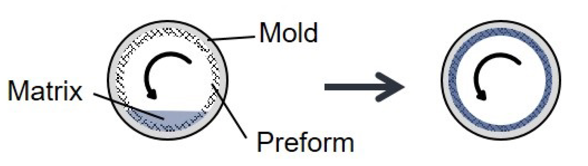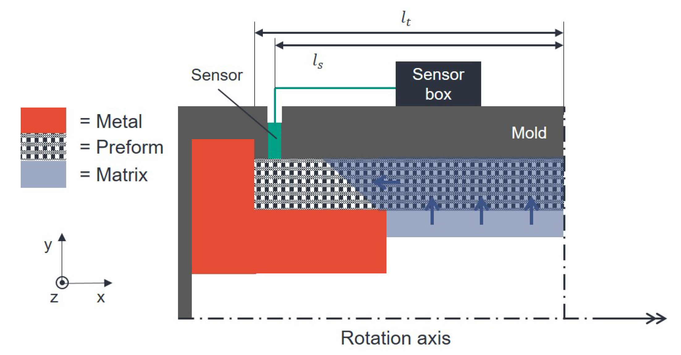Meanwhile, structural components are also manufactured for which a dry perform with continuous fiber reinforcement is used [6,7,8,9]. This preform made of semi-finished products is placed in a mold and impregnated with a matrix under rotation (see Figure 1). The matrix used can be either thermoplastic [6] or thermoset [7,9]. The impregnation pressure is generated by the resulting centrifugal force due to the rotation. Infiltration and curing take place during rotation. After sufficient curing, the component can be removed from the mold with no need of further finishing work.

Compared to established manufacturing processes, metallic load introduction elements can be intrinsically joined in this process. No subsequent joining steps such as bolting, screwing or adhesive bonding are required [9]. The connection between laminate and load introduction element can either be a co-cured or form-fit joint [10,11]. The co-cured joint is based on the adhesive properties of the thermoset matrix used.

Rotational molding, just as RTM or vacuum-assisted resin infusion (VARI), pertains to the liquid composite molding (LCM) processes. Therefore, the cycle time and thus the process costs strongly depend on the time required for infiltration and curing. In addition, it must be ensured that the preform is completely impregnated and that no dry spots occur. In general, the impregnation paths in the rotational molding process are short. As a result, the preform can be fully impregnated and cured in a very short time if heat is applied and low-viscosity matrix systems are used.

Koch [10] developed an analytical model to predict the impregnation with thermoset matrix systems for rotational molding based on the work of Ehleben [6]. The analytical model uses Darcy’s law [12] and calculates the impregnation times as a function of preform permeability [13,14], viscosity and impregnation pressure. The impregnation pressure depends on geometry, rotation speed and volume of matrix used [10].

A disadvantage of this analytical model is the fact that only very simple and no complex geometries with undercuts or polygons can be calculated. In addition, the analytical model cannot take into account multilayer structures with different fiber angles. Furthermore, in Koch’s model, the viscosity is assumed to be constant, and the cure degree is not considered. The cure degree is highly important, since this parameter can be used to determine the time of demolding to ensure that the part is not demolded too early (i.e. uncured) but also not too late (loss of valuable production time).

The current state of research shows different approaches for numerical modeling the LCM processes such as VARI [15,16] or RTM [17,18,19,20,21]. As with analytical calculations, Darcy’s law is used. For the numerical simulation, kinetic, viscosity and permeability must be calculated. The Kamal-Sourour model [22] is often used for kinetics and the Castro-Macosko model [23] for viscosity. 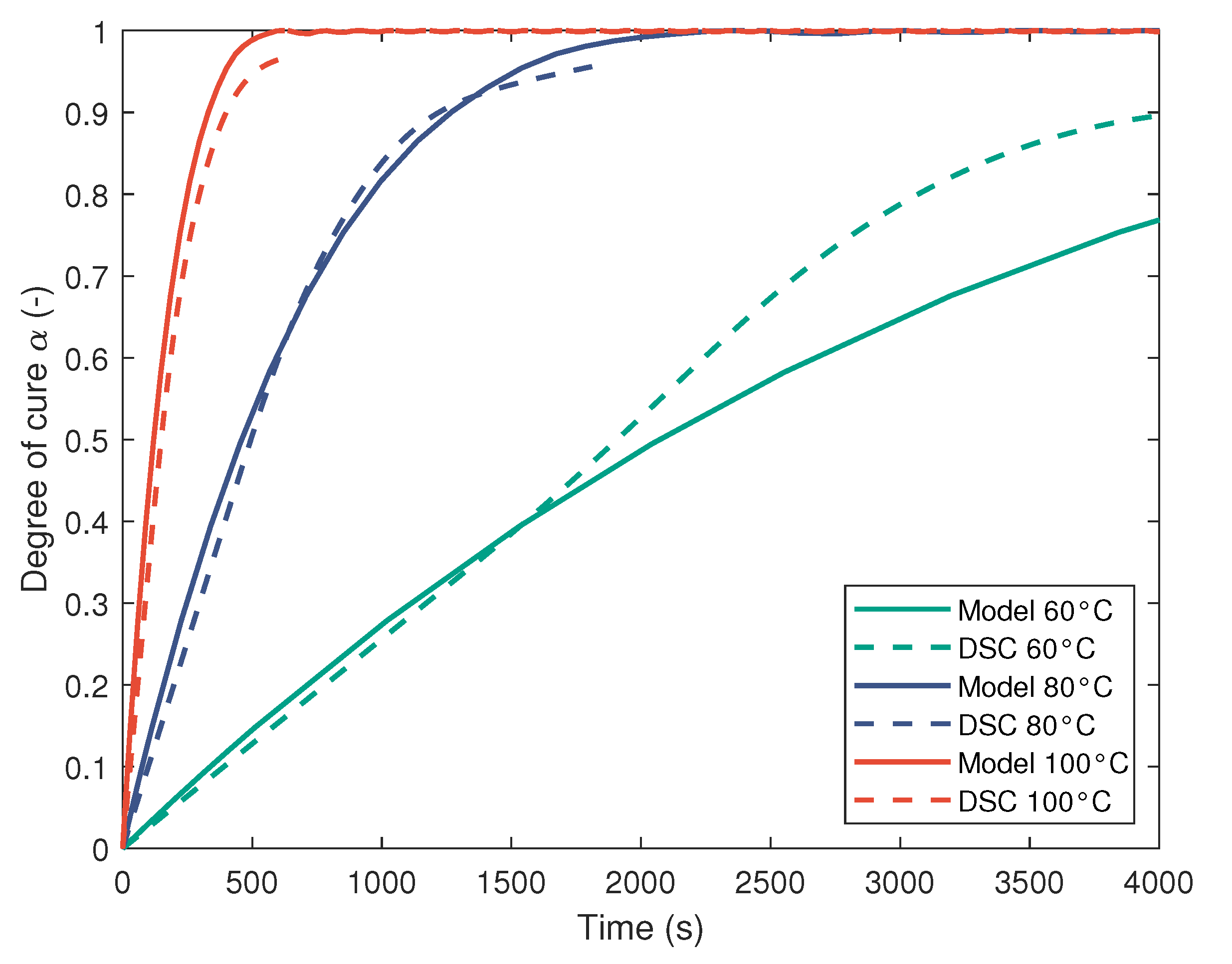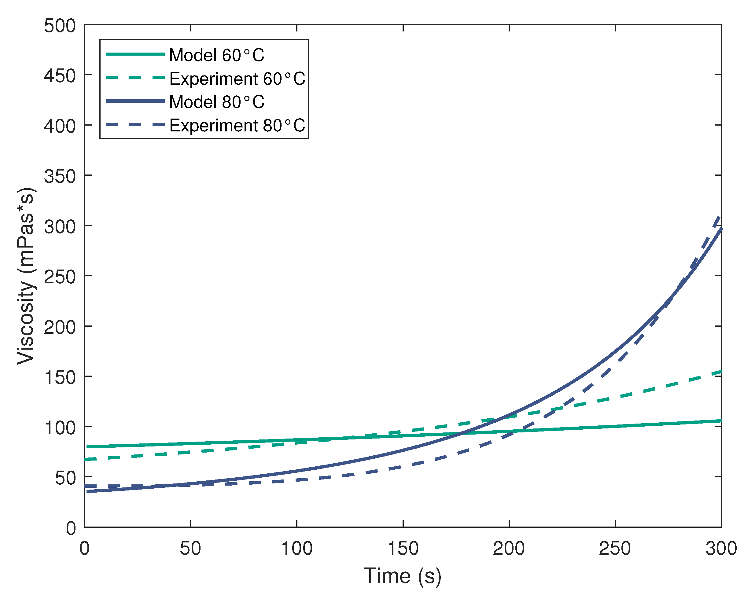In addition, semi-analytical approaches [13] or flow measurements [24] are used to determine permeability. Kinetic and viscosity model are linked via the degree of cure $\alpha$. Isothermal measurements of curing show a faster increase in viscosity at higher temperature. The degree of cure $\alpha$ also increases faster over time at higher temperatures and reaches higher values. Laminates with higher values of $\alpha$ show slightly higher crack initiation stresses [25]. However, depending on the desired mechanical properties, different temperatures and curing cycles can be applied [26].

For the numerical modeling of conventional LCM processes, the commercial programs PAM-RTM or Ansys Fluent are often used. However, they are only specifically suitable for modeling the RTM or VARI process. The rotational molding process differs significantly from the known processes due to the rotating motion. Currently, no approach exists for numerical modeling of the rotational molding process.

Therefore, the objective of this research is to develop a numerical model for the rotational molding process. For the purpose of ensuring the necessary freedom in the implementation of the process, the present approach applies the OpenFOAM© software [27]. Compared to the RTM or VARI process, other boundary conditions must be applied. The viscosity of the matrix system and the permeability of the preform are characterized using experimental data that is fitted to suitable models. To validate the numerical model, a measurement principle is developed and integrated into the rotational molding process. Experimental and simulated results are compared to evaluate the model.

2. Simulation

The rotational molding process with an internal load introduction element is shown in Figure 2. Impregnation of the fiber preform is conducted first mainly in radial direction and then axially to impregnate the overlap area l_o. To ensure complete venting of the laminate and prevent the formation of dry spots, so-called ventilation holes are drilled into the load introduction elements at the end of the overlap area [10].

In the following, the methods used to create the numerical model, the kinetic, viscosity and permeability models, as well as the results obtained from the calculation are presented.

2.1. Methods

2.1.1. Fluid Mechanics and Numerical Methods

In order to simulate the flow of the liquid matrix through the fiber preform, Darcy’s law is applied [12]. The law describes the flow of a liquid through a porous medium, which in this case is the preform:

$$\mathit{v}=-\frac{K}{\mu }·\nabla p$$

(1)

where $\mathit{v}$ is the volume averaged velocity, p the pressure field, $\mu$ the viscosity and $\mathit{K}$ the permability of the preform. In this case the OpenFOAM software is used, which employs a finite volume (FV) approach to solve the Navier-Stokes-Equations. Darcy’s law is added as a source term to the momentum equation [20]. Therefore, the matrix is modeled as a quasi incompressible liquid phase and the air as a compressible gas phase [28]. Magagnato [29] created a model based on OpenFOAM’s interFoam solver to simulate the RTM process. This solver is used and adapted to the rotational molding process.

2.1.2. Implementation of the Rotation

In contrast to the RTM process, rotational molding does not use a press or pump to generate the pressure to impregnate the fibers, but rotation. Therefore, the impact of the rotation has to be added to the simulation. An additional source term is thus added to the momentum equation. The influence of the centrifugal force is calculated by:

$$F_{\mathrm{Cen}}=\rho ·(\mathit{\omega }\times (\mathit{\omega }\times \mathit{r}))$$

(2)

where $\mathit{r}$ is the radius of the respective element, $\mathit{\omega }$ is the angular speed, $\rho$ is the density [27]. The required data are stored in a table, where they can also be changed depending on the time.

2.1.3. Mesh Creation

In order to reduce the number of mesh elements and to achieve an acceptable calculation time, the rotational symmetry around the rotation axis is used as shown in Figure 3. In addition, a symmetry plane is introduced in the center of the considered area. This simplification allows the calculation to be reduced to a two-dimensional simulation case. The calculation time can thus be significantly shortened. The simulation area is marked in red in Figure 3.

The simulation area is decomposed into a mesh, which is divided into two areas (see Figure 4). The first area represents the preform as a porous medium with a corresponding permeability. The second area up to the rotation axis only contains fluid (air/matrix) and therefore no permeability is implemented. In this empty area, the matrix is deposited at the beginning of the simulation. A convergence analysis of the mesh has been carried out and can be found in the Appendix A (see Figure A1). The results show that a number of 9000 cells show the best compromise between low calculation time and high accuracy. The cells of the porous preform have a thickness of 0.3 mm in y direction and a length of approximately 0.40 mm in x direction. The element density in the porous area is set higher, because the simulation has to be more accurate in this area. It is therefore important that the element size increases smoothly and no elements with high aspect ratios exist. However, to reduce the number of cells, a grading of cell thickness in y direction towards the porous media is used, so that the cellsize gets smaller towards the porous area and the mesh is refined locally.

The fiber volume fraction and the orientation of the fibers in the preform significantly influence the permeability and thus the impregnation behavior. Therefore, an anisotropic permeability model is used that takes into account fiber orientation and fiber volume fraction. A two-phase flow of matrix and air is created, which is presented in Figure 5. The matrix is depicted in blue and the air in grey.

2.1.4. Boundary Conditions

For the correct functioning of the model, initial conditions and boundary conditions at the edges of the considered area have to be defined. In this context, the already mentioned symmetry axis (Figure 3 and Figure 4) needs to be addressed. Further inital and boundary conditions are listed in

Table 1. Start and boundary conditions.

	Inlet	Outlet	Walls
Velocity	zero gradient	“inletOutlet”	slip
Resin fraction	uniform 0	zero gradient	zero gradient
Pressure	fixed value = 1 × 105 Pa	fixed value = 1 × 105 Pa	“fixedFluxPressure”
Temperature	fixed value = configuration	fixed value = configuration	fixed value = configuration

. At the outlet, the boundary condition prevents matrix or air from flowing back into the porous media through the outlet. It acts like a membrane which is only permeable in one direction [27]. In addition, one boundary condition is selected at the inlet where air can permanently flow into the simulation area. Fixed values are specified for pressure and temperature. At the walls, a slip boundary condition is set. This condition adds no additional drag and only the Darcy term influences the flow. For flows through porous media with low permeability, the drag of a no-slip wall is negligible compared to the porous drag.

2.2. Material Models

The most relevant material parameters to describe the flow in the rotational molding process are the matrix viscosity and the preform permeability.

2.2.1. Kinetic Model

The viscosity is characterized by using kinetic and viscosity models to model the dependence on temperature and cure degree. Literature offers various models to describe the curing kinetics for epoxy matrix systems [22,30,31]. Since the Kamal-Sourour model [22] is well-known [32,33,34,35,36] and also widely used in commercial programs, it is chosen for the present case. In addition, the effort required for fitting the parameters is acceptable [37]. The equation to describe the degree of cure $\alpha$ is as follows:

$$\frac{\partial \alpha }{\partial t}=(K_1+K_2{\alpha }^m)·{(1-\alpha )}^n$$

(3)

where K1 and K2 are rate constants with an Arrhenius type equation:

$$\begin{array}{c}\hfill K_1=A_1·e^{\left(\frac{-E_1}{R·T}\right)}\end{array}$$

(4)

$$\begin{array}{c}\hfill K_2=A_2·e^{\left(\frac{-E_2}{R·T}\right)}\end{array}$$

(5)

The parameters m and n are catalytic constants, $A_1,A_2$ are pre-exponential factors $E_1,E_2$ are activation energies, R is the gas constant and T the temperature.

In order to determine the parameter values of the Kamal-Sourour model, isothermal and dynamic measurements are performed by differential scanning calorimetry (DSC) with TA Instruments’ Q200 analyzer. The matrix used is Sicomin’s SR8500/SZ8525 epoxy system, which is recommended for hot processes and short cycle times [38]. The dynamic DSC measurements are carried out with heat rates of 1, 2.5, 5, 10 and 15 °C min^-1 from −40 °C to 300 °C. The degree of cure $\alpha$ depends on the enthalpy released during the DSC measurement and is determined by formula:

$$\begin{array}{c}\hfill \alpha =\frac{h\left(t\right)}{\Delta h}=\frac{1}{\Delta h}·{\int }_{t_0}^{t}q\left(\widehat{t}\right)d\widehat{t}\end{array}$$

(6)

where $\Delta h$ is the total heat of reaction and $q\left(\widehat{t}\right)$ is heat flow at time t. The total heat of reaction $\Delta h$ is calculated by determining a baseline under the exothermic peak and integrating the enclosed area. With the results of the five dynamic DSC measurements, a mean of $\Delta h$ is computed.

For the isothermal runs, measurements are conducted at 60 °C, 80 °C, 100 °C. The samples are quickly mixed and placed in the DSC analyzer, which has already been preheated to the appropriate temperature. After no more heat is released, the samples are rapidly cooled and then heated to 300 °C at a defined heating rate of 10 °C min⁻¹ in order to calculate the residual heat of reaction. With this residual heat and $\Delta h$, the curves are determined and fitted with the nonlinear least-squares algorithm, as shown in Figure 6. The required prediction of the fitted Kamal-Sourour model agrees well with the isothermal DSC data, only the slope towards the end of the curves is not accurately reproduced because the DSC measurements do not reach a final value of $\alpha$ = 1.

Table 2. Area difference between DSC measurement and Kamal-Sourour model predictions.

	60 °C	80 °C	100 °C
Area DSC	2530.2	1218.1	475.0
Area model	2194.4	1210.8	484.8
Deviation	13.27 %	0.6 %	−2.06 %

shows the area difference between the experimental DSC results and the Kamal-Sourour model prediction. The model prediction for 60 °C shows the largest deviation from the DSC measurement. In addition, it can be seen that the matrix is not fully cured even after 4000 s at 60 °C, so that tests at 60 °C require a correspondingly long time. This is a well-known phenomenon at low constant temperatures [33,39]. To achieve a complete cure of 100 % ($\alpha$ = 1), it is recommended to post-cure the matrix. In

Table 3. Parameter values for the Kamal-Sourour kinetic model fitted to isothermal DSC data.

Parameter	Value	Unit ()
m	7.431	-
n	7.527 × 10−1	-
$A_1$	1.100 × 108	s${}^{-1}$
$A_2$	−9.543 × 105	s${}^{-1}$
$E_1$	7.369 × 104	J$·$mol${}^{-1}$
$E_2$	5.713 × 1010	J$·$mol${}^{-1}$
R	8.314	J$·$(mol$·$K)${}^{-1}$

the parameter values for the fitted Kamal-Sourour model are given.

2.2.2. Viscosity Model

The frequently used Castro-Macosko model [19,33,36] is selected for the time-dependent viscosity $\eta$. The model is defined as follows [23]:

$$\eta (T,\alpha )={\eta }_0\left(T\right)·{\left(\frac{{\alpha }_{\mathrm{g}}}{{\alpha }_{\mathrm{g}}-\alpha }\right)}^{(c_1+c_2·\alpha )}$$

(7)

with the initial viscosity ${\eta }_0\left(T\right)$ at $\alpha =0$:

$${\eta }_0\left(T\right)=A_{\eta }·e^{\left(\frac{E_{\eta }}{R·T}\right)}$$

(8)

where $\alpha$ is the degree of cure, ${\alpha }_{\mathrm{g}}$ the degree of cure at gelation, T the temperature , R the gas constant and $A_{\eta },B_{\eta },c_1,c_2$ the fitting parameters. The viscosity measurements are provided by the datasheet of the manufacturer [38]. The focus of the fitting lies upon the time period crucial for the rotational molding process with values below 300 s. Figure 7 shows a comparison between the values predicted with the Castro-Macosko model and the experimentally measured values of the datasheet. The corresponding parameter values are presented in

Table 4. Parameters values for the Castro-Macosko viscosity model.

Parameter	Value	Unit ()
$A_{\eta }$	4.633 × 10−5	Pa$·$s
$E_{\eta }$	3.978 × 104	J$·$mol${}^{-1}$
$c_1$	1.603	-
$c_2$	2.737	-
R	8.314	J$·$(mol$·$K)${}^{-1}$
${\alpha }_{\mathrm{g}}$	0.63	-

.

2.2.3. Permeability Model

The permeability of the fiber preform is described by the Koch model [10], which is largely based on the model of Gebart [13]. In this model, the fiber bundles are represented as an ellipsoid, since the fiber bundles are usually not ideally round in shape, as showed in Figure 8. The equivalent radius $r_{\mathrm{eq}}$ of the fiber bundles used in this study is calculated using the equation according to van West et al. [14]:

$$r_{\mathrm{eq}}=\sqrt{2}·\frac{a_0{b}_0}{\sqrt{a_0^2+b_0^2}}$$

(9)

with $2a_0$ being the length of the ellipsoid and $2b_0$ being the width of it.

In general, permeability can be divided into longitudinal permeability, which is parallel to the fibers and transverse permeability, which is orthogonal to the fibers. With the radius $r_{\mathrm{eq}}$, the longitudinal permeability $K_{\Vert }$ is calculated by [13]:

$$K_{\Vert }=\frac{8r_{\mathrm{eq}}^2}{c}\frac{{(1-{\phi }_{\mathrm{f}})}^3}{{\phi }_{\mathrm{f}}}$$

(10)

The following equation describes the transversal permeability $K_{\perp }$ [13]:

$$K_{\perp }=C_1{\left(\sqrt{\frac{{\phi }_{\mathrm{f}},\max }{{\phi }_{\mathrm{f}}}}-1\right)}^{\frac{5}{2}}·r_{\mathrm{eq}}^2$$

(11)

where ${\phi }_{\mathrm{f}}$ is fiber volume fraction and $C_1,c,{\phi }_{\mathrm{f}},\max$ are constants, which depend on the packing order (square, hexagonal or mixed) of the preform [10,13].

In the rotational molding process, depending on the fiber orientation, it often occurs that a mixed state between longitudinal and transverse permeability in axial direction (x axis) exists Figure 9. Axial permeability is the permeability along the axis of rotation. Therefore, an extended model is applied [10,40], which considers longitudinal and transverse permeability according to their proportions:

$$K_{xx}=K_{\Vert }{cos}^2\beta +K_{\perp }{sin}^2\beta$$

(12)

In order to calculate the permeability of the used braided sleeves, computer tomographic scans are taken at the wbk Institute of Production Science by using a Metrotom 800 CT-scanner from Carl Zeiss. The software VGStudio Max is used to measure the dimensions of the fiber bundles by manual thresholding using the grey-scale values. A total of 24 different rovings are analyzed and the fiber volume fraction ${\phi }_{\mathrm{f,macro}}$ of 12 different scans is determined using automatic grey scale analysis. In addition, the fiber angle $\beta$ of the preform is determined. The parameters to calculate the permeability can be taken from

Table 5. Parameters for the permeability calculation.

	Mean Value	Deviation
$C_1$	$\frac{1}{2}·(\frac{16}{9·\pi ·\sqrt{2}}+\frac{16}{9·\pi ·\sqrt{6}})$	-
c	55	-
${\phi }_{\mathrm{f,macro}}$ (%)	65.24	±2.621
${\phi }_{\mathrm{f,max}}$	$\frac{1}{2}·(\frac{\pi }{4}+\frac{\pi }{2·\sqrt{3}})$	-
$a_0$ (mm)	2.1	±0.219
$b_0$ (mm)	0.29	±0.044
$\beta$	42.5 °	±2.5

.

These values are then used to calculate the mean value for permeability as well as the maximum and minimum permeability based on the corresponding standard deviation. The obtained parameter values are listed in

Table 6. Permeability values for axial permeability (x-direction) and radial permeability (y-direction).

	Axial Permeability	Radial Permeability
Mean	2.5280 × 10−10	9.3585 × 10−11
Maximum	5.9832 × 10−10	2.3608 × 10−10
Minimun	1.3098 × 10−10	4.4764 × 10−11

.

3. Experiments

The experiments pursue the objective of validating the developed model for the rotational molding process through tests with different manufacturing parameters. The challenge is that, compared to conventional processes such as RTM or VARI, only wireless sensors can be used and the imbalance of the mold resulting from the components must be compensated. For validation, the time at which the sensor detects the matrix is compared with the numerically calculated time for reaching this point.

Set-Up

In order to obtain a high impregnation pressure at moderate rotational speeds, a large mold with an outer diameter of the component of 80 mm is selected (see Figure 10). Due to the high total mass of the rotational mold, the additional mass due to the sensor technology is less significant. Nevertheless, an axisymmetric balance weight must be fixed to ensure sufficiently high rotation speeds and to avoid vibrations.

For the detection of the matrix, either pressure [41], capacitive [42] or point-voltage sensors [43] have been considered. Initial tests with a pressure sensor [41] have shown that the impregnation pressure in the rotational molding process is not sufficiently high for a defined measurement signal. This is also indicated by the simulation results, which show a pressure increase to only 1.02 bar. Therefore, a capacitive sensor [42] of Rechner Sensors is subsequently used. The disadvantage of capacitive and point-voltage sensors is that they can only be used with glass fibers and not with electrically conductive carbon fibers. The validation experiments are thus carried out using glass fiber preforms.

Since a cable-guided power supply is not possible, the electrical supply of the capacitive sensor is ensured by a series connection of 9 V rechargeable batteries (see Figure 11). The sensor is embedded into the mold and connected to a Raspberry 4 8 GB single-board computer. Raspberry then transmits the signal wirelessly via WiFi to a measurement computer for further steps. Except for the sensor, all electronics are housed in a box that is attached to the mold (see Figure 10 and Figure 12). The distance of the sensor from the center of the mold $l_s$ is 67.5 mm.

For the experimental tests, the preforms are first built up. Each preform consists of seven layers of glass fiber braided sleeves with ø 80 mm [44] (see

Table 7. Manufacturing parameters.

Parameter	Value
Number of preform layers	7
Preform material	Glassfibers [44]
Binder	EPIKOTE 05390 [45]
Heating temperature oven and water bath	≈60 °C and ≈80 °C
Heating time	1 h
Matrix	SR8500/ SZ8500 [38]
Mean value matrix quantity	108.38 g
Rotation speed	800 RPM and 1200 RPM
Time required for mixing	≈30 s

). To prevent the preform from collapsing when placed into the mold, a binder powder [45] is applied between the layers and activated by temperature. The preform is then placed into the mold together with the metallic load introduction elements and sealing elements. To ensure a homogeneous temperature of the mold across all surfaces, the mold is heated in an oven for one hour. In parallel, resin and hardener are also heated in a water bath to the respective test temperature. After heating in the oven, the mold is removed, and the sensor box is swiftly attached to the mold. Resin and hardener are quickly mixed and placed into the mold. The amount of matrix added to the mold is measured with a precise digital scale. For the simulations the mean value of the quantity of matrix is used (see Table 7). The mold is then clamped in an Index IT 600 lathe and rotated at the specified speed (see Figure 10). The time required for mixing the matrix until the rotation starts is approximately 30 s.

4. Results

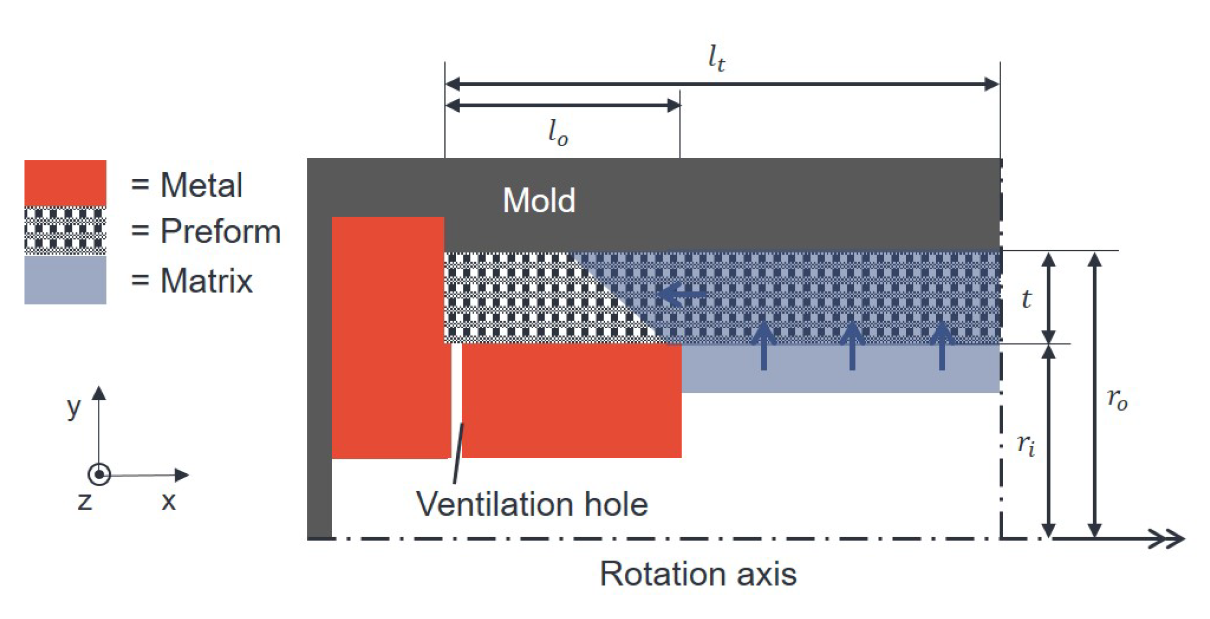
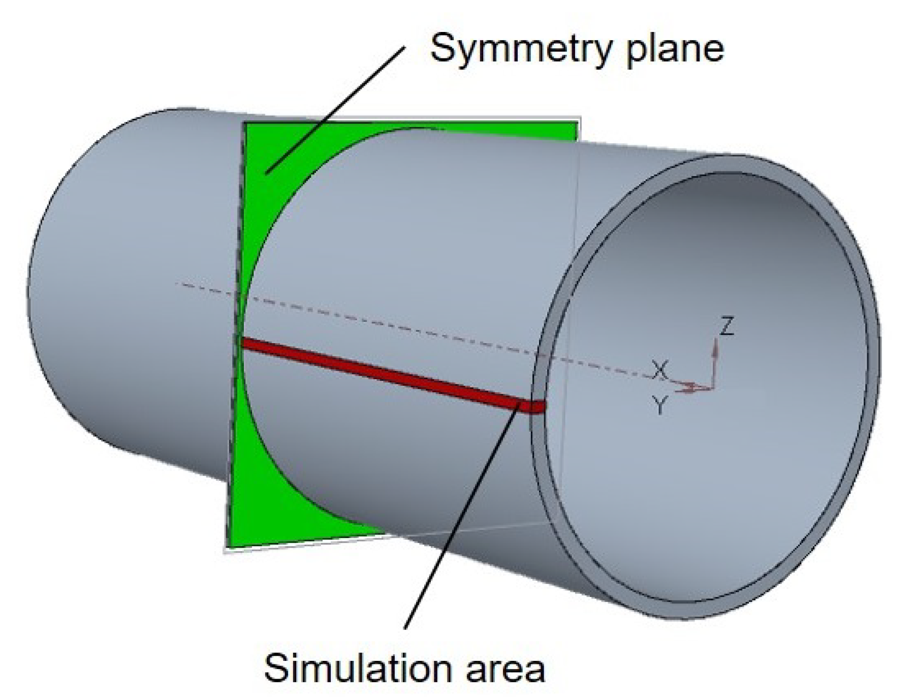
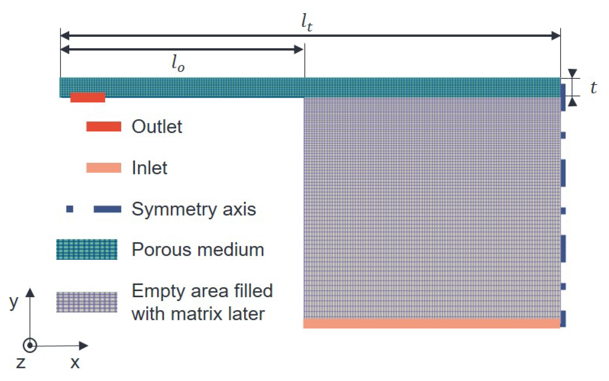
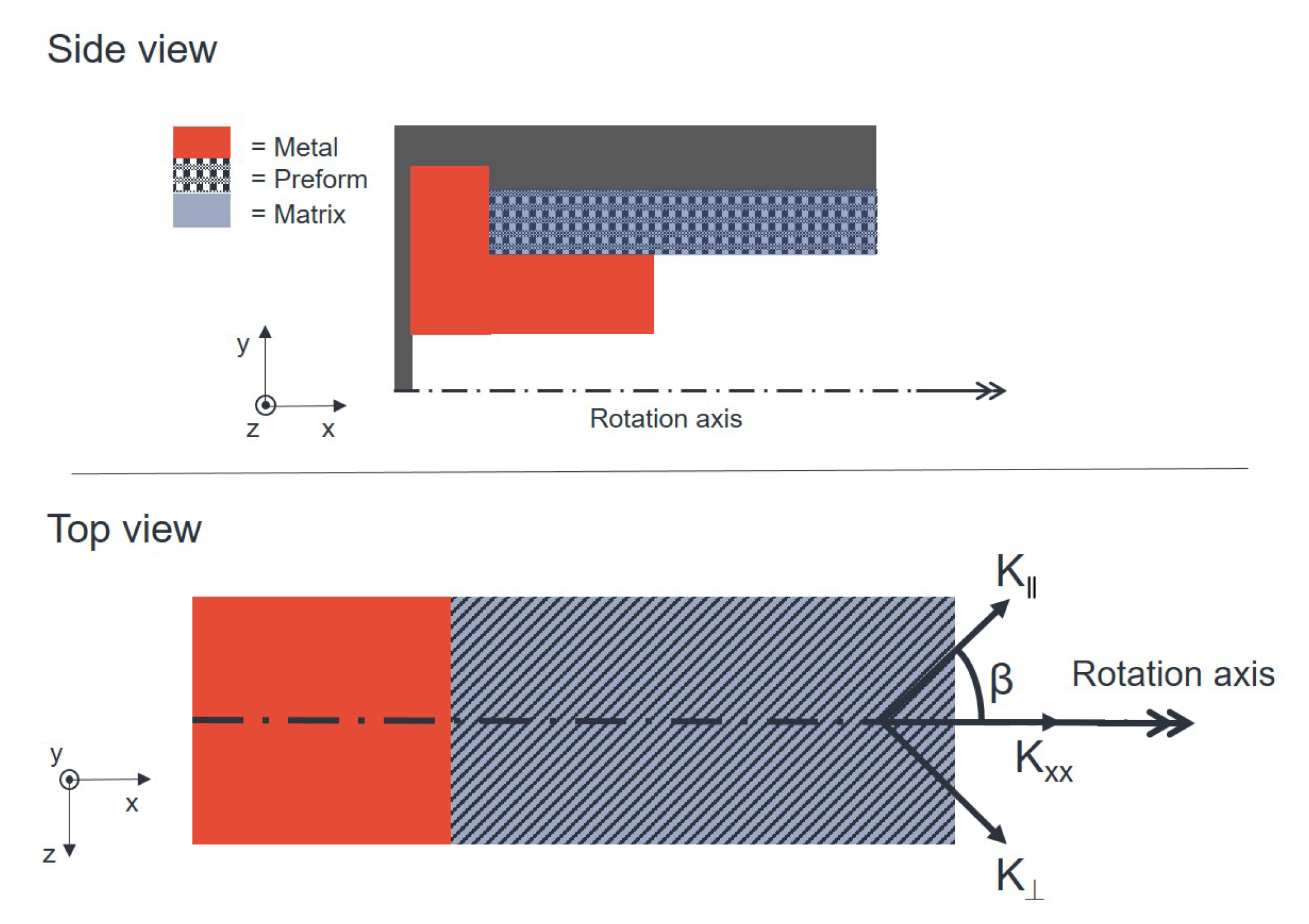
Using the developed numerical solver for the rotational molding process, a simulation is performed in OpenFOAM. For this purpose, the corresponding area from Figure 3 and Figure 4 is considered. The size of the simulation model equals the validation geometry. The overlap length between laminate and load introduction element is 40 mm and the thickness of the preform is 3 mm (see

Table 8. Mold dimensions.

Parameter	Value	Unit ()
Overlap length $l_{\mathrm{o}}$	40	mm
Total length $l_{\mathrm{t}}$	82.5	mm
Thickness t	3	mm
Inner radius $r_{\mathrm{i}}$	37	mm
Outer radius $r_{\mathrm{o}}$	40	mm

). The temperature specified is 60 °C, which is particularly important for the adapted kinetic model and also for the viscosity model. A speed of 1200 RPM is set for the rotation and the values for axial and radial permeability from Section 2.2.3 are placed in the solver.

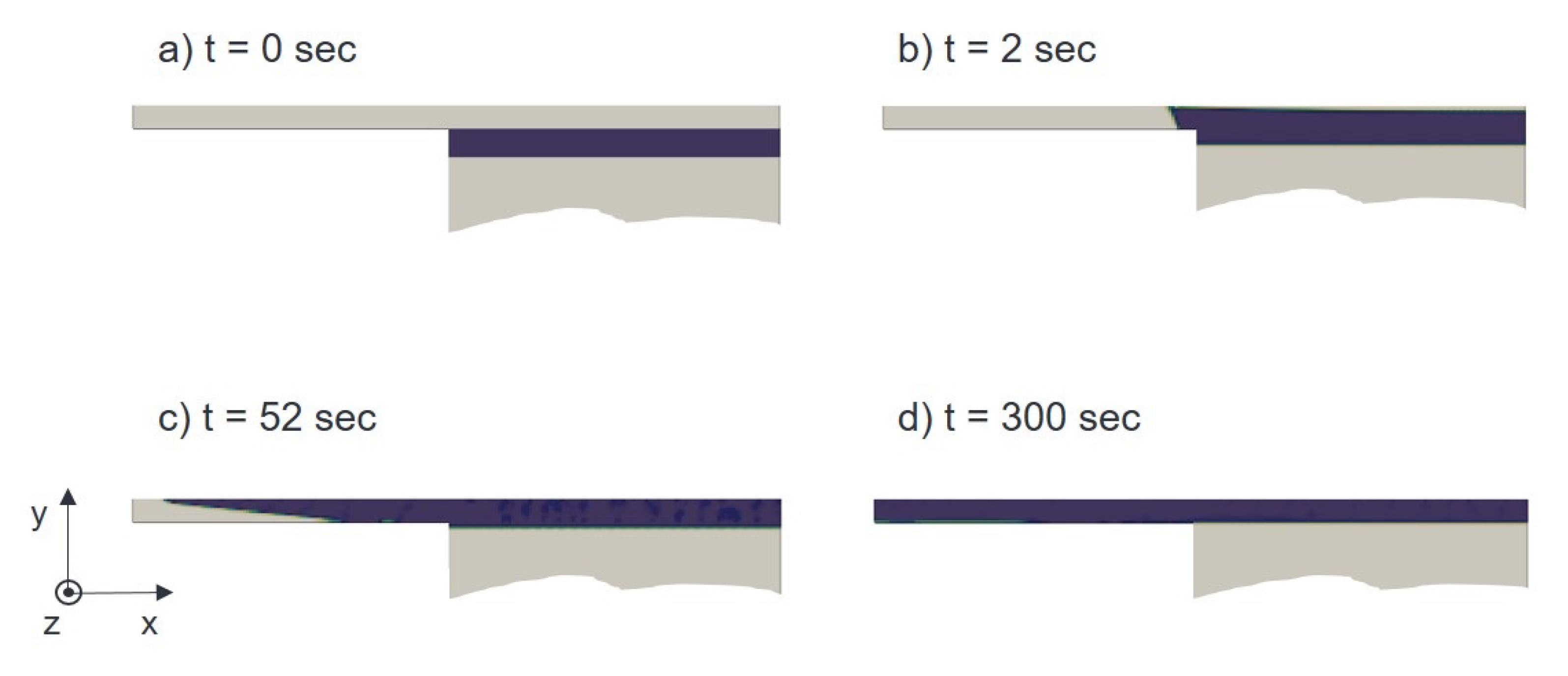
Different stages of the impregnation are illustrated in Figure 13. At t = 0 s, the matrix is introduced into a region without permeability and there is no rotation yet. It can be observed that the radial impregnation (y direction) of the preform takes place very quickly at the parameters used and is almost complete at t = 2 s. Axial impregnation requires considerably more time and is preceded by a flow front on the inside of the mold (Figure 13c).

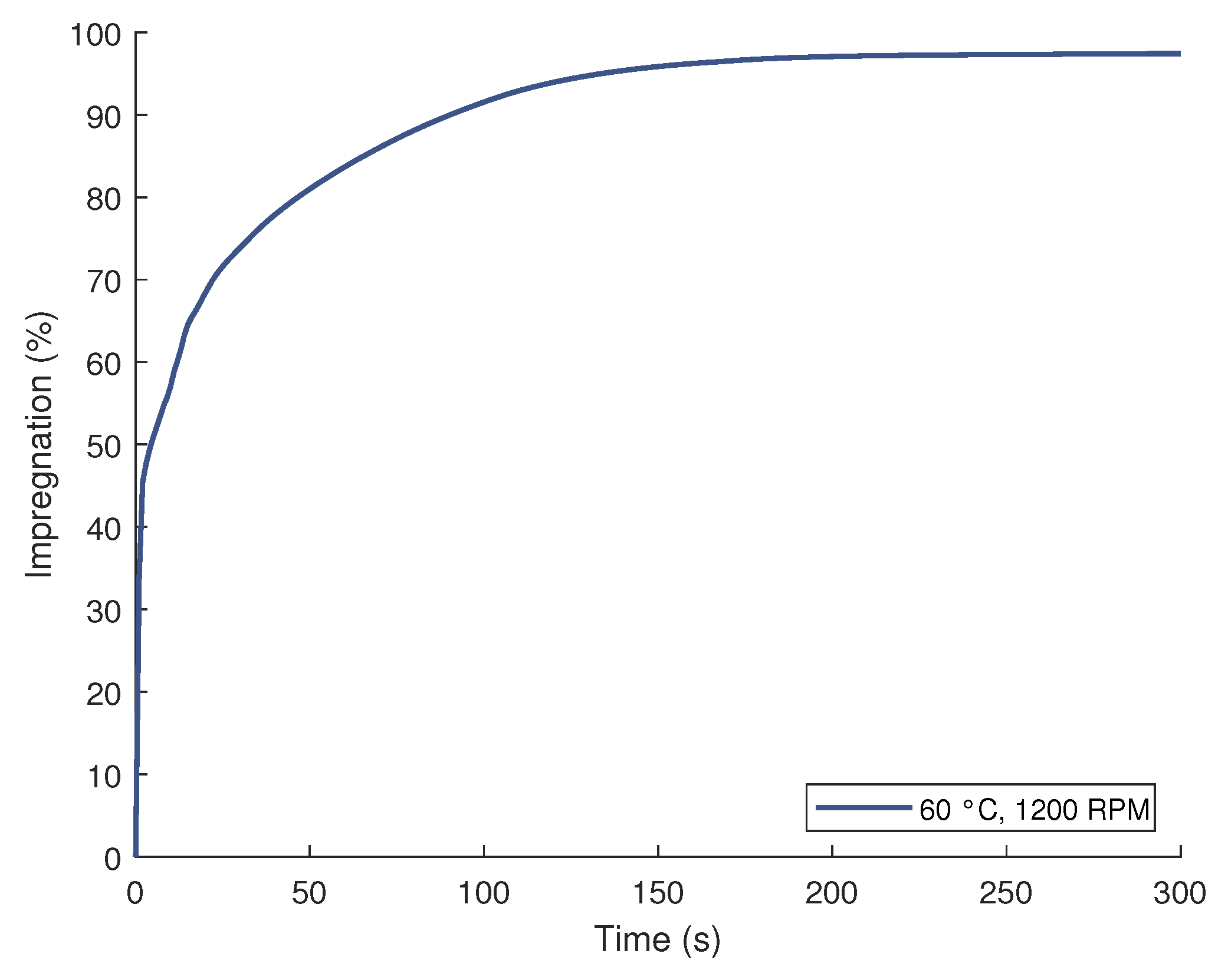
Figure 14 shows the impregnation process over time. A value of 100% means that the volume of the preform to be filled is completely impregnated. The simulation results demonstrate that 100% impregnation cannot be fully achieved with the used parameters. This is consistent with the findings from real experiments, where it is found that a small matrix excess is always required for generating sufficient pressure to ensure complete impregnation of the preform and good surface quality [10].

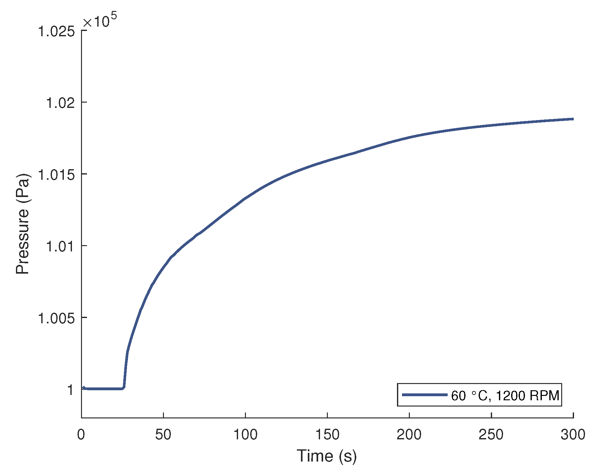
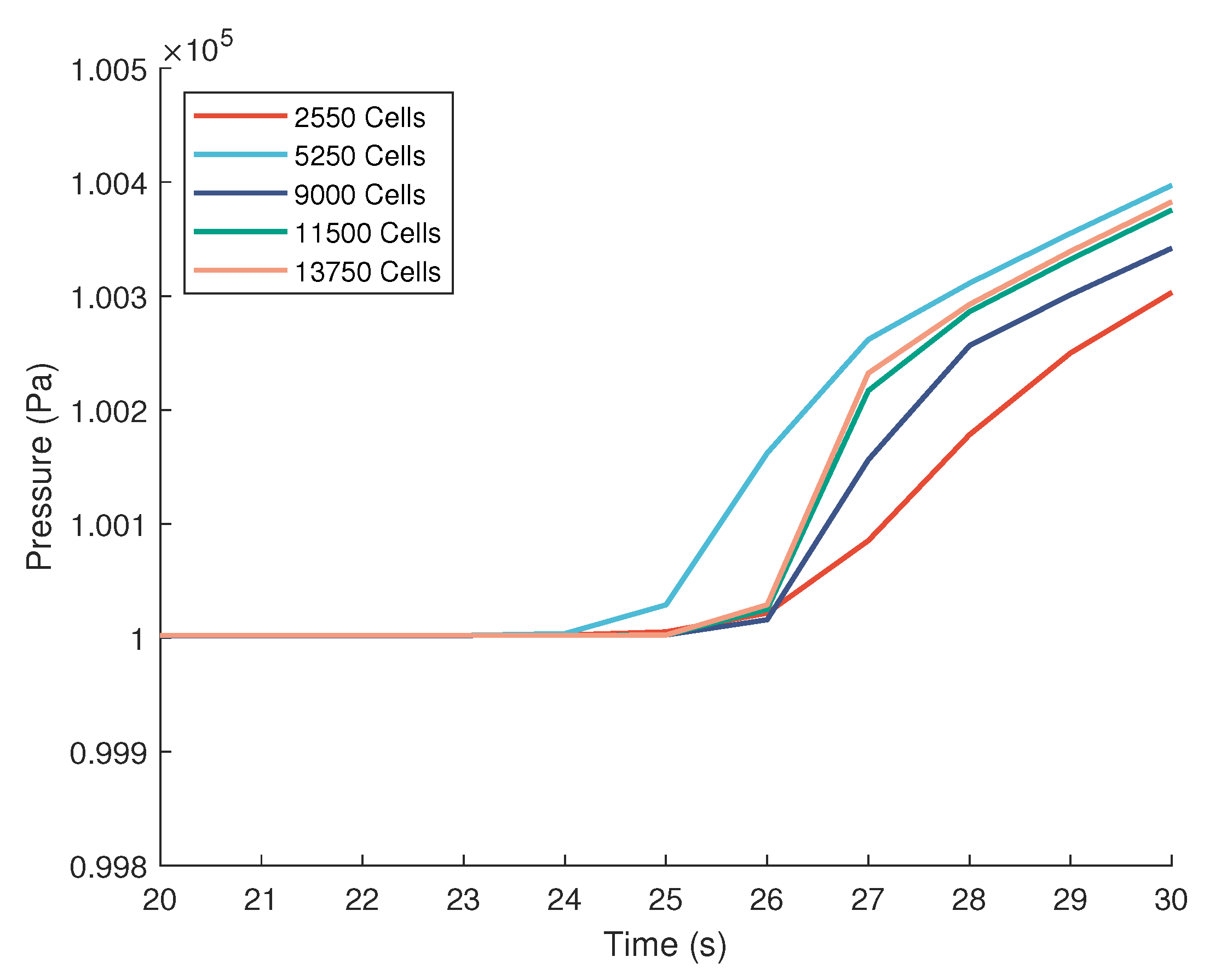
To compare the numerical simulation and the experiment, the position of the sensor was analyzed considering the pressure. The first pressure increase in the simulation is important (see Figure 15), being the time to be compared with the time of the sensor deflection from the experiment. The mold only cools very slowly once it has been removed from the oven until the sensor signal is received due to the large mass. Its cooling is thus not considered in the simulation.

In order to compare and validate the model in a large parameter space, four different configurations are defined (see

Table 9. Configuration parameters.

Configuration	Temperature (°C)	Rotation Speed (RPM)
1	60	800
2	60	1200
3	80	800
4	80	1200

). Temperature and rotation speed are varied. The two parameters are deliberately chosen low because it is very difficult to measure short impregnation times with the developed experimental setup. The structure of the preform is not changed. Four experimental measurements are conducted with the sensor for each configuration and the mean value and standard deviation are calculated subsequently.

As with all experiments, there is some scatter in the process parameters. These parameters comprise the temperature, the time for mixing the matrix and starting the rotation, and the axial as well as the radial permeability (see

Table 10. Lower and upper simulation limits.

	Lower Limit (Faster) Impregnation Time	Upper Limit (Slower)
Temperature	+3 °C	−3 °C
Start of rotation	−3 s	+3 s
Radial Permeability	2.36 × 10−10	4.48 × 10−11
Axial Permeability	5.98 × 10−10	1.31 × 10−10

). Depending on the type of scattering, the time until the sensor detects the matrix can be either reduced or increased. As a result, two limits can be distinguished for the impregnation time on the basis of the scattering: A lower limit (faster) and an upper limit (slower) (see Table 10). For example, higher temperature and quick mixing decrease the viscosity of the matrix, accelerating impregnation. Lower permeability, on the other hand, increases flow resistance and slows down impregnation. Thus, for each configuration, an additional simulation is performed with the fastest and slowest limits, respectively.

The results of this comparison are shown in Figure 16. Each configuration is indicated on the x axis whereas the respective time that the matrix needs to reach the sensor or the time which is calculated simulatively in OpenFOAM is presented on the y axis. The mean values of the experiments are shown as diamonds, while the mean values of the simulation are shown as squares. The error bars for the experiments represent the standard deviation and the error bars for the simulation represent the fastest and slowest impregnation (see limits in Table 10).

The longest impregnation time for reaching the sensor is measured for variant 1 at 60 °C and 800 RPM. The simulation of this variant predicts a slightly shorter impregnation time.

Table 11. Deviations of simulation results and measured mean values for reaching the sensor.

	Variant 1	Variant 2	Variant 3	Variant 4
Experiment	69.3 s	14.0 s	49.8 s	18.3 s
Simulation	60.0 s	24.0 s	30.0 s	12.0 s
Deviation	15.4%	−41.7%	65.8%	52.1%

shows the percentage deviations of simulation results and measured values. In the present case, the deviation between simulation and experiment is 15.4%. The measured standard deviation falls within the simulated limits for the fastest or slowest impregnation time. Increasing the speed of rotation in variant 2 to 1200 RPM reduces the measured time to reach the sensor by more than half. Here, the lower standard deviation lies outside the simulated lower limit. The deviation between simulated and measured mean value is −41.7%. In variant 3, a higher temperature of 80 °C and a rotational speed of 800 RTM are specified. Compared to variant 1, the measured impregnation time is reduced. This can be explained by the lower viscosity due to the higher temperature. However, due to the lower rotational speed, the time is higher than the one of variant 2. For variant 4 with 80 °C and 1200 RPM, the time decreases significantly compared to variant 3. However, the measured mean value is higher than the one for variant 2 (60 °C and 1200 RPM). Here, a shorter time than that for variant 2 was expected due to the higher temperature. The devation between simulated and measured mean value is 52.1%. Overall, the absolute times measured at high rotational speeds are extremely low, so that even small deviations during measurement have a large influence on the result.

It can be seen that the discrepancy between mean values of experiments and simulation is small, varying between twenty and six seconds depending on the configuration. The deviations are between −41.7%–65.8%. Overall, this results in an average deviation of 43.8%. In the simulation, shorter impregnation times are calculated, except for configuration 2. The higher temperature and speed, the lower the scatter of the measurements.

A comparison of numerical and experimental results reveals that the standard deviations of the experiments and the fastest and slowest impregnation time simulations overlap (except for configuration 2). All mean values of the experiments are within the calculated limits of the simulation. This qualitative trend can be considered as a validation of the presented numerical model.

The results also demonstrate that lower impregnation times can be achieved both with an increase in rotation as well as an increase in temperature, whereby the selected temperature depends on the respective matrix and the number of rotations on the balance quality of the loaded mold.

5. Conclusions

This work pursued the objective of implementing a numerical model for the impregnation of dry fiber preforms in the rotational molding process. For this purpose, an existing RTM mold filling simulation method is extended and permeability, kinetic and viscosity models are selected and adapted. Comparisons between measurements and numerical results confirm the high quality of the developed model.

Hence, the numerical model can be used to calculate the impregnation progress for the rotational molding process and the time required for complete mold filling. Simulations demonstrate that radial impregnation occurs extremely quickly, whereas axial impregnation consumes a larger part of the time required. By increasing the viscosity-influencing temperature and the rotation speed, the impregnation time can be significantly reduced. In addition, other matrix systems, geometries or braided sleeves with smaller filament bundles can easily be integrated into the model by adjusting the parameters.

The model also considers the curing degree of the thermoset matrix. In future studies, this will be used to determine the optimum time for demolding. Thus, too early demolding with an uncured component, but also too late demolding with the loss of valuable production time should be prevented.

References

1. Heuss, R.; Müller, N.; van Sintern, W.; Starke, A.; Tschiesner, A. Lightweight, Heavy Impact: How Carbon Fiber and Other Lightweight Materials Will Develop across Industries and Specifically in Automotive; Project Report for McKinsey & Company: London, UK, 2012. [Google Scholar]
2. Lubin, G. Handbook of Composites; Springer Science & Business Media: Berlin/Heidelberg, Germany, 2013. [Google Scholar]
3. Fleischer, J.; Teti, R.; Lanza, G.; Mativenga, P.; Möhring, H.C.; Caggiano, A. Composite materials parts manufacturing. CIRP Ann. 2018, 67, 603–626. [Google Scholar] [CrossRef]
4. Rost, A. Epoxyd-Gießharzmassen für das Schleuderguß-Verfahren. Kunststoffe 1965, 55, 96–99. [Google Scholar]
5. Dürkop, J.; Maihart, H. Das Rotations-Harz/Faser-Spritzverfahren: Ein wirtschaftliches Verfahren zum Herstellung von Behältern und Silos aus GFK. Kunststoffe 1973, 63, 564–569. [Google Scholar]
6. Ehleben, M.; Schürmann, H. Manufacturing of centrifuged continuous fibre-reinforced precision pipes with thermoplastic matrix. Compos. Sci. Technol. 2006, 66, 2601–2609. [Google Scholar] [CrossRef]
7. Fleischer, J.; Koch, S.F.; Coutandin, S. Manufacturing of polygon fiber reinforced plastic profiles by rotational molding and intrinsic hybridization. Prod. Eng. 2015, 9, 317–328. [Google Scholar] [CrossRef]
8. Fleischer, J.; Koch, S.F.; Ruhland, P. Rotational molding of fiber reinforced plastics with elastic composite core. In Proceedings of the International Conference on Competitive Manufacturing, Resource Efficiency for Global Competitiveness, Stellenbosch, South Africa, 27–29 January 2016; pp. 181–186. [Google Scholar]
9. Koch, S.F.; Barfuss, D.; Bobbert, M.; Groützner, R.; Riemer, M.; Stefaniak, D.; Wang, Z. Intrinsic Hybrid Composites for Lightweight Structures: New Process Chain Approaches; Advanced Materials Research; WGP Congress 2016; Trans Tech Publications Ltd.: Stafa-Zurich, Switzerland, 2016; Volume 1140, pp. 239–246. [Google Scholar] [CrossRef]
10. Koch, S.F. Fügen von Metall-Faserverbund-Hybridwellen im Schleuderverfahren: Ein Beitrag zur fertigungsgerechten Intrinsischen Hybridisierung; Shaker: Düren, Germany, 2017. [Google Scholar]
11. Nieschlag, J.; Coutandin, S.; Fleischer, J.; Production and Tensile Testing of Rotationally Molded Hybrid Composite Tie Rods. SAMPE 2020 Virtual Series|Multifunctional Materials and Structures. 2020. Available online: https://www.nasampe.org/store/viewproduct.aspx?id=16320936 (accessed on 25 October 2021).
12. Darcy, H.P.G.; Les Fontaines Publiques de la ville de Dijon. Exposition et Application des Principes à Suivre et des Formules à Employer dans les Questions de Distribution d’eau, etc. Available online: https://discover.libraryhub.jisc.ac.uk/search?ti=Les%20fontaines%20publiques%20de%20Dijon&rn=2 (accessed on 25 October 2021).
13. Gebart, B.R. Permeability of unidirectional reinforcements for RTM. J. Compos. Mater. 1992, 26, 1100–1133. [Google Scholar] [CrossRef]
14. Van West, B.P.; Pipes, R.B.; Advani, S.G. The consolidation of commingled thermoplastic fabrics. Polym. Compos. 1991, 12, 417–427. [Google Scholar] [CrossRef]
15. Malheiro, J.M.; Nunes, J.P. Simulation of Vacuum Assisted Resin Infusion (VARI) process for the production of composite material parts. In Advances in Evolutionary and Deterministic Methods for Design, Optimization and Control in Engineering and Sciences; Springer: Cham, Switzerland, 2021; pp. 319–340. [Google Scholar] [CrossRef]
16. Zhao, C.; Zhang, G.; Wu, Y. Resin flow behavior simulation of grooved foam sandwich composites with the vacuum assisted resin infusion (VARI) molding process. Materials 2012, 5, 1285–1296. [Google Scholar] [CrossRef]
17. Deléglise, M.; Le Grognec, P.; Binetruy, C.; Krawczak, P.; Claude, B. Modeling of high speed RTM injection with highly reactive resin with on-line mixing. Compos. Part A Appl. Sci. Manuf. 2011, 42, 1390–1397. [Google Scholar] [CrossRef]
18. Grössing, H.; Stadlmajer, N.; Fauster, E.; Fleischmann, M.; Schledjewski, R. Flow front advancement during composite processing: Predictions from numerical filling simulation tools in comparison with real–world experiments. Polym. Compos. 2016, 37, 2782–2793. [Google Scholar] [CrossRef]
19. Trochu, F.; Ruiz, E.; Achim, V.; Soukane, S. Advanced numerical simulation of liquid composite molding for process analysis and optimization. Compos. Part A Appl. Sci. Manuf. 2006, 37, 890–902. [Google Scholar] [CrossRef]
20. Seuffert, J.; Kärger, L.; Henning, F. Simulating mold filling in Compression Resin Transfer Molding (CRTM) using a three-dimensional finite-volume formulation. J. Compos. Sci. 2018, 2, 23. [Google Scholar] [CrossRef] [Green Version]
21. Han, S.H.; Cho, E.J.; Lee, H.C.; Jeong, K.; Kim, S.S. Study on high-speed RTM to reduce the impregnation time of carbon/epoxy composites. Compos. Struct. 2015, 119, 50–58. [Google Scholar] [CrossRef]
22. Kamal, M.R.; Sourour, S. Kinetics and thermal characterization of thermoset cure. Polym. Eng. Sci. 1973, 13, 59–64. [Google Scholar] [CrossRef]
23. Castro, J.M.; Macosko, C.W. Studies of mold filling and curing in the reaction injection molding process. AIChE J. 1982, 28, 250–260. [Google Scholar] [CrossRef]
24. Grössing, H.; Becker, D.; Kaufmann, S.; Schledjewski, R.; Mitschang, P. An evaluation of the reproducibility of capacitive sensor based in-plane permeability measurements: A benchmarking study. Express Polym. Lett. 2015, 9. [Google Scholar] [CrossRef]
25. Ozaki, T.; Kosaka, T.; Kusukawa, K. Effect of Degree of Cure on Damage Development in FRP. In Fracture, Fatigue, Failure and Damage Evolution, Volume 8; Springer: Berlin/Heidelberg, Germany, 2016; pp. 27–33. [Google Scholar]
26. Singh, S.B.; Vummadisetti, S.; Chawla, H. Influence of curing on the mechanical performance of FRP laminates. J. Build. Eng. 2018, 16, 1–19. [Google Scholar] [CrossRef]
27. OpenCFD Ltd. OpenFOAM: User Guide v1912; OpenCFD Ltd.: London, UK, 2020. [Google Scholar]
28. Magagnato, D.; Seuffert, J.; Bernath, A.; Kärger, L.; Henning, F. Experimental and numerical study of the influence of integrated load transmission elements on filling behavior in resin transfer molding. Compos. Struct. 2018, 198, 135–143. [Google Scholar] [CrossRef]
29. Magagnato, D.; Bernath, A.; Henning, F. Experimentelle und numerische Untersuchung der Infiltration bei der RTM-Fertigung. Verbundwerkstoffe Und Werkst. 2013, 511–517. [Google Scholar] [CrossRef]
30. Henne, M.; Breyer, C.; Niedermeier, M.; Ermanni, P. A new kinetic and viscosity model for liquid composite molding simulations in an industrial environment. Polym. Compos. 2004, 25, 255–269. [Google Scholar] [CrossRef]
31. Grindling, J. Simulation zur Verarbeitung von Reaktiven Non-Post-Cure-Epoxidharz-Systemen im Druckgelieren und konventionellen Vergießen; Shaker: Düren, Germany, 2006. [Google Scholar]
32. Ruiz, E.; Waffo, F.; Owens, J.; Billotte, C.; Trochu, F. (Eds.) Modeling of Resin Cure Kinetics for Molding Cycle Optimization. 2006. Available online: https://ecm-academics.plymouth.ac.uk/jsummerscales/FPCM/FPCM08/FPCM8/papers/FPCM8_18.pdf (accessed on 25 October 2021).
33. Garschke, C.; Parlevliet, P.P.; Weimer, C.; Fox, B.L. Cure kinetics and viscosity modelling of a high-performance epoxy resin film. Polym. Test. 2013, 32, 150–157. [Google Scholar] [CrossRef]
34. Lee, C.L.; Ho, J.C.; Wei, K.H. Resin Transfer Molding (RTM) process of a high performance epoxy resin. I: Kinetic studies of cure reaction. Polym. Eng. Sci. 2000, 40, 929–934. [Google Scholar] [CrossRef]
35. Shojaei, A.; Ghaffarian, S.R.; Karimian, S.M.H. Three-dimensional process cycle simulation of composite parts manufactured by resin transfer molding. Compos. Struct. 2004, 65, 381–390. [Google Scholar] [CrossRef]
36. Wittemann, F.; Maertens, R.; Bernath, A.; Hohberg, M.; Kärger, L.; Henning, F. Simulation of reinforced reactive injection molding with the finite volume method. J. Compos. Sci. 2018, 2, 5. [Google Scholar] [CrossRef] [Green Version]
37. Bernath, A.; Kärger, L.; Henning, F. Accurate cure modeling for isothermal processing of fast curing epoxy resins. Polymers 2016, 8, 390. [Google Scholar] [CrossRef] [PubMed]
38. Sicomin. Datasheet: SR 8500/SZ 8525 Fast and Clear Epoxy System for Hot Processes. 2021. Available online: http://sicomin.com/composite-datasheets-and-downloads/epoxy-systems/fast-curing (accessed on 25 October 2021).
39. Karkanas, P.I.; Partridge, I.K.; Attwood, D. Modelling the cure of a commercial epoxy resin for applications in resin transfer moulding. Polym. Int. 1996, 41, 183–191. [Google Scholar] [CrossRef]
40. Endruweit, A.; Long, A.C. Analysis of compressibility and permeability of selected 3D woven reinforcements. J. Compos. Mater. 2010, 44, 2833–2862. [Google Scholar] [CrossRef]
41. Kistler. Datasheet: Typ 4001A Cavity Pressure Sensor for Low-Pressure RTM with Front ø9 mm. 2021. Available online: https://www.kistler.com/en/product/type-4001a/ (accessed on 25 October 2021).
42. Rechner Sensors. Datasheet: Capacitive Sensors: Series 70—NPN, Series 80—PNP. 2021. Available online: https://www.rechner-sensors.com/wp-content/uploads/2018/07/KAT-KAS-EN_.pdf (accessed on 25 October 2021).
43. Danisman, M.; Tuncol, G.; Kaynar, A.; Sozer, E.M. Monitoring of resin flow in the resin transfer molding (RTM) process using point-voltage sensors. Compos. Sci. Technol. 2007, 67, 367–379. [Google Scholar] [CrossRef]
44. Bacuplast. Datasheet: Glass Fiber Braided Sleeves Nr. 10.080 80 mm. 2021. Available online: https://www.bacuplast-shop.de/epages/61604045.sf/de_DE/?ObjectPath=/Shops/61604045/Categories/Glasfaser/Glasfaserschlauch/%22Glasfaserschlauch%20Nr.10.080%22 (accessed on 25 October 2021).
45. Hexion. Datasheet: Binder Powder EPIKOTE 05390. 2021. Available online: https://www.hexion.com/CustomServices/PDFDownloader.aspx?type=tds&pid=03a5863b-5814-6fe3-ae8a-ff0300fcd525 (accessed on 25 October 2021).
Figure 1. Simplified representation of the rotational molding process with thermoset matrix.
Jcs 05 00289 g001
Figure 2. Impregnation in the rotational molding process [10].
Jcs 05 00289 g002
Figure 3. Simplified simulation with symmetry plane and rotation axis.
Jcs 05 00289 g003
Figure 4. Mesh for the simulation case.
Jcs 05 00289 g004
Figure 5. Two-phase flow with matrix and air at the start of rotational molding.
Jcs 05 00289 g005
Figure 6. Degree of cure α as a function of time fitted to isothermal DSC data.
Jcs 05 00289 g006
Figure 7. Comparison between viscosity η as a function of time of the Castro-Macosko model and the experimental measurements.
Jcs 05 00289 g007
Figure 8. Determination of the equivalent radius of the fiber bundles r eq by computed tomography studies of the cross section.
Jcs 05 00289 g008
Figure 9. Axial permeability based on [10].
Jcs 05 00289 g009
Figure 10. Mold for the rotational molding process and finished component.
Jcs 05 00289 g010
Figure 11. Electrical circuit diagram with capacitive sensor.
Jcs 05 00289 g011
Figure 12. Sensor integration into the mold.
Jcs 05 00289 g012
Figure 13. Different stages of impregnation for 60 °C and 1200 RPM.
Jcs 05 00289 g013
Figure 14. Impregnation progress over time.
Jcs 05 00289 g014
Figure 15. Simulated pressure curve at the position of the sensor after starting the rotation.
Jcs 05 00289 g015
Figure 16. Comparison of the experimentally measured times with the numerically calculated times for reaching the sensor with the matrix.
Jcs 05 00289 g016