
Efficient Finite Element Modeling of Steel Cables in Reinforced Rubber


Designing Plastics and Composite Materials, Department of Polymer Engineering and Science, Montanuniversitaet Leoben, 8700 Leoben, Austria
*
Author to whom correspondence should be addressed.
J. Compos. Sci. 2022, 6(6), 152; https://0-doi-org.brum.beds.ac.uk/10.3390/jcs6060152
Submission received: 3 March 2022
/
Revised: 17 May 2022
/
Accepted: 20 May 2022
/
Published: 24 May 2022
(This article belongs to the Special Issue Characterization and Modelling of Composites, Volume II)
Abstract
:Spiral steel cables feature complex deformation behavior due to their wound geometry. In applications where the cables are used to reinforce rubber components, modeling the cables is not trivial, because the cable’s outer surface must be connected to the surrounding rubber material. There are several options for modeling steel cables using beam and/or solid elements for the cable. So far, no study that lists and evaluates the performance of such approaches can be found in the literature. This work investigates such modeling options for a simple seven-wire strand that is regarded as a cable. The setup, parameter calibration, and implementation of the approaches are described. The accuracy of the obtained deformation behavior is assessed for a three-cable specimen using a reference model that features the full geometry of the wires in the three cables. It is shown that a beam approach with anisotropic beam material gives the most accurate stiffness results. The results of the three-cable specimen model indicate that such a complex cable model is quite relevant for the specimen’s deformation. However, there is no single approach that is well suited for all applications. The beam with anisotropic material behavior is well suited if the necessary simplifications in modeling the cable–rubber interface can be accepted. The present work thus provides a guide not only for calibrating but also for selecting the cable-modeling approach. It is shown how such modeling approaches can be used in commercial FE software for applications such as conveyor belts.
1. Introduction
Steel cables are an indispensable part of the infrastructure and many engineering applications because they reliably provide high strengths with low bending stiffness. They consist of individual steel wires that are wound into strands, which in turn are wound to form the cable. Since cables consist of many parallel thin wires, their tensile stiffness is very high, whereas the bending and compressive stiffness are low. Because of this helical topology of spiral cables, there is a coupling of tensile deformation and torsional deformation of the cable (see Figure 1). Steel cables have many design options in terms of steel grade and cable geometry. Much work has been done on computing the influence of those parameters on the cable stiffness, accounting for the trajectories of the individual wires and contact between them. Many analytical and semi-analytical solutions have been developed and are listed in the review papers by Utting and Jones [1], Cardou and Jolicoeur [2], and the works of Costello [3] and Feyrer [4]. For standard cable types, good agreement of existing cable models with experiments can be reached. Effects like wire–wire friction can be captured. Hysteresis effects, the nonlinearity of the cable stiffness, and cable failure have been studied as well. Most of the work of such cable models is setting up the geometry, particularly for a non-straight cable; see Wang et al. [5]. Recently, the finite element method (FEM) has become widely used for modeling the mechanical response of cables: Jiang et al. [6] modeled a seven-wire strand using cyclic symmetry, and Foti and de Luca di Roseto [7] investigated the elastic–plastic effects of the wires. Furthermore, FEM provides a basis for newly developed simplified models; see Chen et al. [8] and Cao and Wu [9].
Many of the mathematical cable models refer to tests of a seven-wire strand reported by Utting and Jones [10], who reported a distinct tension/torsion coupling. When testing cables, the constraints of the cable ends influence the test results. The cable ends can be free, clamped, or even welded together. This effect of the cable ends was studied by Chen et al. [11] for thick cables, and they showed that in cable tests and FEM simulations of cables, much care must be put into applying the loads.
Modeling steel cables in reinforced rubber on the one hand requires capturing the influence of the rubber penetrating the cable (see Bonneric et al. [12]). On the other hand, the outer surface of the cable needs to be connected to the rubber. This interface between cable and rubber is crucial for the failure of cable-reinforced rubber components, as modeled by Frankl et al. [13].
Cable-reinforced rubber components can be conveyor belts, for example; see Nordell [14], Fedorko et al. [15], and Frankl et al. [16]. Obtaining the stiffness of cables that are used in rubber components requires tests on cables that have been penetrated by rubber (rubberized cables). How to separately capture tensile, bending, and torsion stiffness and the tension/torsion coupling of the cable that is embedded in rubber is a big challenge. Nordell et al. [17] stated that they developed a special element in the commercial FEM code ANSYS based on principles described by Costello [3], but did not give any details about this element.
In the present work, a variety of such cable modeling approaches is evaluated for their use in rubber components using the commercial FEM code Abaqus [18]. Those efficient modeling approaches use solid elements, beam elements, or a combination of both. In some of those modeling approaches, an anisotropic material model is used to mimic the tension/torsion coupling of the cable. To not have to deal with uncertainties of tests, the results of a fully modeled rubberized cable are taken as the reference to evaluate the accuracy of these modeling approaches. In this reference model, all wires and the surrounding rubber are modeled with a linear elastic and a hyperelastic material model, respectively. This model is called a full-geometry model, in contrast to the efficient models that account for wires and rubber in a way such that the overall cable stiffness is captured.
To keep the computational cost low, a seven-wire rubberized strand is used as the cable. For this cable, the homogenized stiffness matrix is computed from a full-geometry simulation similar to what was reported by Cartraud and Messager [19]. The various cable-modeling approaches are then calibrated and their ability to capture the homogenized stiffness components of the full-geometry model is evaluated. Then, the modeling approaches are evaluated in a simple rubber shear specimen containing three cables. The loads applied in these specimens are similar to those in conveyor belts; see Nordell et al. [17]. The full-geometry version of the three-cable specimen is used as a reference, and the stiffness, deformation, and strains in the specimen are used to assess the performance of the efficient models.
2. Methods
This section introduces the homogenized cable stiffness and a range of efficient modeling approaches that attempt to mimic this stiffness matrix . The cables are regarded as linear elastic throughout this study. For typical cable loads, this is a good approximation despite the nonlinear elastic response of the rubber. This section further describes the setup of the single-cable FEM model that computes the matrix for a seven-wire rubberized strand and is used to calibrate and evaluate efficient cable-modeling approaches. Additionally, a FEM model of a three-cable specimen is introduced, which is used to evaluate the performance of the efficient cable models.
2.1. Cable Stiffness
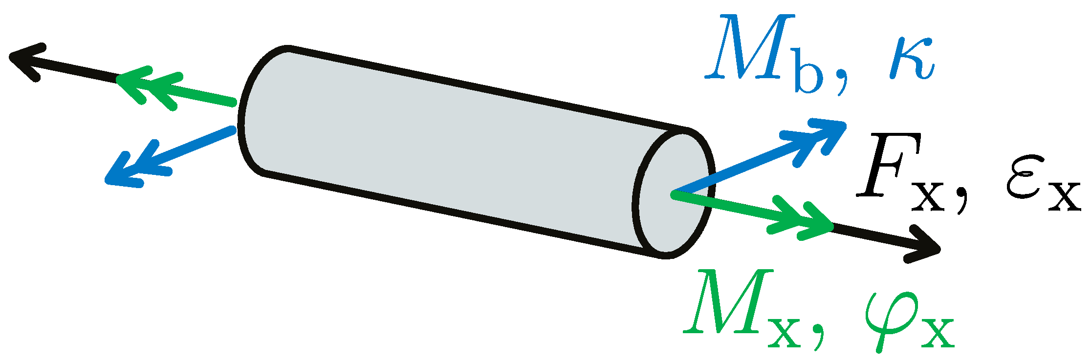
Figure 2 illustrates the loads (normal load , twist moment , and flexural moment ) and corresponding deformations (longitudinal strain , twist per length , and curvature ) of a cable, which is drawn as a cylinder. Longitudinal shear deformation is not considered and the elastic bending response is considered to be independent of the bending direction.
Since we regard small deformations, the stiffnesses in tension and compression and the stiffness for positive and negative twist are assumed to be the same. The elastic behavior of the cable can then be described by a stiffness matrix (or ) that couples the loads and deformations as
with defined as
Inverting the stiffness matrix yields the compliance matrix (or ). Similar to the definition of Young’s modulus, we define stiffness parameters of the cable , , …, which correspond to the inverse of the components of :
If all non-diagonal terms vanish (all terms except , , and are zero), the values , , and are the same as , , and , respectively. If this is not the case, it means that is the longitudinal stiffness that is observed when twist and bending strains are constrained during loading. On the other hand, corresponds to the longitudinal stiffness when twist and bending are free ( and are zero).
Let us assume that we have a cable that has off-diagonal terms, which means that tension, twist, and bending are coupled. When we use an efficient cable model that cannot account for those coupling terms, we can fit either , , and or , and . In the first case, the modeled cable has the same stiffness as the real cable when all other strains are set to zero during loading. For tension, this means that torsion and curvature are constrained during loading. When fitting , , and , the efficient cable model shows the same stiffness as the real cable during loading in one direction when strains in the other directions are unconstrained.
For an FEM model of a cable, the cable’s stiffness matrix can be obtained by applying three orthogonal strain vectors similar to [19]. The stiffness matrix can be built from the resulting load vectors. If the applied strains , , and are set to 1, the resulting load vectors constitute the columns of the stiffness matrix. Otherwise, the terms of the stiffness matrix must first be divided by the applied strain.
2.2. Cable-Modeling Approaches
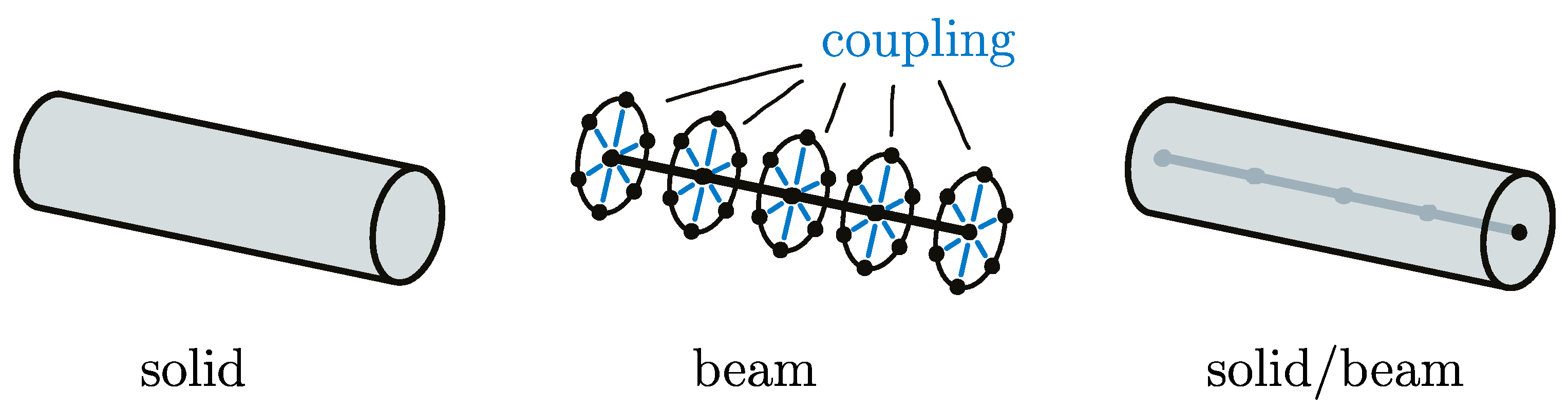
The cables can be modeled either by using solid elements that share nodes with the surrounding rubber, by using a beam that is coupled in some way to the corresponding rubber nodes, or with a combination of solid and beam elements (see Figure 3). The nodes of the beam in the solid/beam approach cannot transmit rotation since a direct nodal connection is used and the solid element nodes do not have rotational degrees of freedom. Each option requires a specific calibration of material parameters. These parameters are not physical but selected such that the whole modeled cable captures the target elastic response.
Our efficient cable-modeling approaches aim to reach , , , and as closely as possible (Section 3.1 will show that and can generally be neglected). Some simplified approaches are also investigated that do not account for the coupling term .
The first challenge is to independently capture the tensile and bending stiffness. This can be done in the following ways:
- (a)
- Solid elements: Use a material that has different tensile and compressive stiffness.
- (b)
- Beam elements: Set the radius of the beam such that and fit the target values.
Solid/beam approach: The whole bending stiffness is captured by the solid elements, whereas beam elements are used to capture the tensile stiffness that is not captured by the solid elements; see [16]. The beam elements have a very small cross-section such that the high tensile stiffness does not affect the overall bending stiffness.
In the following, the cable-modeling approaches are presented and their material parameters are derived. For a linear elastic material model with cubic symmetry, the Young’s modulus E, the shear modulus G, and the Poisson’s ratio can be selected independently. For all models with linear elastic material, is set to zero in order to avoid unphysical effects in the cable deformation.
To account for the tension/torsion coupling of the cable, the linear elastic cubic material can be extended to a special kind of anisotropy that couples and in the cylindrical coordinate system of the cable:
The parameter accounts for the coupling of and . Whereas and are taken from the analytical calculations, is calibrated to reach the target value of the efficient cable model. If is set to zero, the coupling vanishes and the model corresponds to cubic material symmetry, with independent values of E and G, and the Poisson’s ratio is set to zero, as in the cubic approach. This linear elastic material model is suited for both solid elements and beam elements. Alternatively, a hyperelastic material model with anisotropic stiffness is used in the solid models. This hyperelastic modeling approach can account for both the tension/torsion coupling and the tensile and bending stiffness and is introduced in the next section.
The material parameters of the homogenization approaches can be calculated analytically or calibrated using FEM models. The analytical calculations are based on the equations for a beam with circular cross-section and radius . The tensile stiffness , torsional stiffness , and bending stiffness of the beam can be written as
The elastic material parameters for the beam, solid, and solid/beam approaches are derived in the following. There, the components are written in the equations. To fit with the homogenized cable (see Section 2.1 for details), the terms in the formulas can be replaced by the corresponding terms, which then, of course, yields the corresponding stiffness for unconstrained loading.
2.2.1. Solid Approaches
There are two types of solid element approaches, where the material model is (a) linear elastic (with either cubic or anisotropic material symmetry) or (b) hyperelastic with anisotropic material response using the Holzapfel–Gasser–Ogden (HGO) formulation. For linear elastic material, the Young’s modulus and shear modulus of the material can be computed directly from the target values of tensile stiffness and torsional stiffness as
This approach results in a bending stiffness that can be computed using the cable radius R by
This means that for the solid approach with cubic material, the axial stiffness and the torsional stiffness can be made to fit while the bending stiffness is too high. The tension/torsion coupling can be captured when the anisotropic linear elastic material is chosen and the previously introduced coupling term is calibrated.
The solid approach can account for , , , and when a material model with anisotropic behavior and a difference in its tensile and compressive stiffness is used. One such model is the Holzapfel–Gasser–Ogden (HGO) material model [20,21], which considers a hyperelastic matrix material model with fiber reinforcements. The HGO matrix uses the neo-Hookean model parameter ; the parameters and define the stiffness of the reinforcements. The parameter defines the level of dispersion of the fiber directions and lies between 0 for uniaxial orientation and 1/3 for evenly distributed fiber orientations. In the HGO model, the reinforcements only increase the stiffness of the material in the fiber direction under tension, but not under compression. It thus provides the possibility to reach a lower bending stiffness with solid elements, in contrast to the linear elastic anisotropic modeling approach. For this modeling approach, is set to zero to model uniaxial reinforcement. The parameter is an additional parameter to account for nonlinear effects and is set to in this work. The parameter D of the HGO model is set to zero, which is equivalent to incompressible material behavior. This deviates from the linear elastic cable models where is set to 0. Since, compared to the rubber, there are only small deformations in the cables, this inconsistency is expected to have a negligible effect on deformations and stresses. Within this HGO approach, the cable is modeled by solid elements and the orientation of the reinforcements is defined to be wound similar to the strands in a cable with a helix angle . Note that this of the HGO model approach can differ from the actual helix angle of the cable since it is calibrated to fit the stiffness components of the cable. The fitting parameters of the HGO approach, therefore, are this helix angle the material stiffness parameters of the matrix , and the stiffness parameter of the reinforcements .
2.2.2. Beam Approaches
When the cable is modeled using beam elements, the beam radius r can be used to also fit the bending stiffness of the cable. To that end, the equations for and can be formulated for the two unknowns, E and r:
After eliminating r by inserting Equation (12) into Equation (13), the Young’s modulus can be written as
This expression for E can be inserted into Equation (12) to yield the beam radius r:
Using Equation (10), the shear modulus of the beam can be calculated from the radius r and the desired as
This means that the beam approach can capture , , and by adjusting , , and . Furthermore, can be captured using a calibrated of the linear elastic material model.
2.2.3. Solid/Beam Approaches
For a combination of solid and beam elements, the Young’s modulus of the solid elements is calculated from the bending stiffness:
The shear modulus follows directly from the torsional stiffness; see Equation (10).
A beam radius is applied to the beam elements, which is a factor of 1000 smaller than the actual cable radius. Thus, the contribution of the beam elements to the torsional and bending stiffness can be neglected. The Young’s modulus for the beam elements is chosen such that the combination of solid stiffness and beam stiffness add up to the desired longitudinal stiffness :
2.3. Single Cable Models
In this section, two kinds of single cable models are introduced. The first is a model with fully modeled steel wires and rubber. This model is used to obtain the cable stiffness matrix , which serves as a reference for the other models. The modeling with steel wires and rubber is referred to as full geometry in the following. The second kind of single cable models are the efficient cable models, which are set up to mimic the reference stiffness using solid elements, beam elements, or a combination of both.
The load definition and the computation of the stiffness are the same for the full-geometry cable model and the efficient single cable models. At the center of the two ends of the modeled cable, reference points are defined. All nodes of the two end surfaces (or end nodes in the case of the beam models) are rigidly coupled to the corresponding reference point. The load is applied at the right-side reference point while the left-side reference point is completely fixed. This constraint of the radial displacements introduces an additional stiffness to the model. It thus must be checked whether the modeled cable length is long enough for the influence of these end effects to vanish. The models are analyzed using the implicit nonlinear solver of Simulia Abaqus [18].
2.3.1. Full-Geometry Single-Cable Model
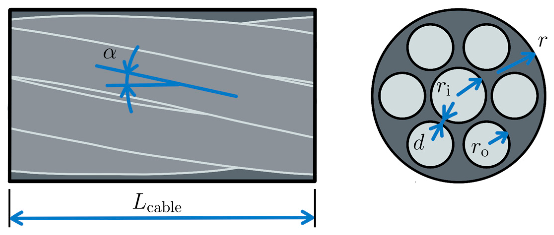
The full-geometry cable model uses a seven-wire rubberized strand as a very simple example of a cable. The strand geometry is defined in Figure 4 and Table 1. It is adapted from [7], but to provide a good-quality mesh [12], the rubber gap between the middle wire and the outer wires is increased. The steel of the wires is modeled linear elastically using a Young’s modulus as given in [7], E = 188 GPa, and Poisson’s ratio = 0.3; the helix angle of the strand is 11.8°. A perfect bond between the rubber and the steel wires is modeled (they share the same nodes in the interface) such that there can be no debonding or friction. The rubber is modeled as a Mooney–Rivlin hyperelastic material model with its parameters , , and taken from [22] as 0. MPa, 0. MPa, and 0. MPa, respectively. The full-geometry single-cable model uses two meshing options: (a) bilinear hexahedral elements with hybrid formulation (C3D8H) for the rubber elements and reduced integration (C3D8R) for the steel elements and (b) quadratic tetrahedral elements with hybrid formulation (C3D10H) both for rubber and steel elements.
The strand length of a cable is the axial distance at which one wire is completely wound around the cable axis. This length depends on the helix angle and the distance between the cable axis and the axis of the wire. In the case of the seven-wire strand used, the strand length of the six outer wires is calculated as
The wires in the strand can be wound in two directions, referred to as the z-type and the s-type, where z is wound like a right-hand screw and s like a left-hand screw. All single cable models use the z-type (see Figure 4) and for the efficient models of s-cables needed in the tree-cable specimen, of the z-type cable is multiplied by −1.
2.3.2. Efficient Single-Cable Models
As stated in Section 2.2, the efficient cable models can be divided into approaches that use cubic material models and approaches that use some kind of anisotropic material response. The latter can be implemented using a linear elastic or hyperelastic material model to account for the tension/torsion coupling of the cables. For both the cubic and anisotropic approaches, cable models consisting of beam elements, solid elements, or both solid and beam elements can be set up. Table 2 defines the combinations of elements and material models used in this study.
The grey areas in Table 2 indicate the combinations that had not been implemented. The hyperelastic material model is used for solid elements only. The solid/beam does not use anisotropic solid material because there, the solid elements represent only a small part of the cable’s tensile stiffness. This means that the tension/torsion coupling could not be achieved. The solid/beam approach does not use anisotropic material for the beam because the beam rotation cannot be transmitted through the nodes they share with the solid elements.
The parameters for the efficient cable models ( for the anisotropic solid and beam models and all parameters of the HGO model) are derived as described in Section 2.2. The calibration procedure of those parameters uses a Nelder–Mead algorithm [23]. For the length of the efficient single-cable models, 40% of the strand length (40% of 118.8 mm) have proven to be sufficient and the global mesh size is set to 1 mm. In the longitudinal direction, the length of the elements is set to 3 mm. For the anisotropic approaches that can feature tension/torsion coupling, components are used to obtain the model parameters. Note that for the solid and beam model, is calibrated to best fit . With the solid HGO approach, all four components are used for the calibration. Although more increments are needed for convergence in the HGO approach, the resulting force and moment curves are approximately linear within the modeled load range. To ensure that the minimum found for the HGO approach in the calibration procedure is not a local one, three starting points of the , , and parameters are evaluated: 600 MPa, 10,000 MPa, 5°; 600 MPa, 26,500 MPa, 11°; and 500 MPa, 10,000 MPa, 20°. They all yield approximately the same results as those stated in Section 3.2. The efficient single cable models are meshed by bilinear hexahedral elements with hybrid formulation (C3D8H) for the solid regions and linear beam elements (B31) for the beams.
2.4. Model of the Three-Cable Specimen
The cable modeling approaches are assessed using an FEM model of a three-cable shear specimen. The geometry and boundary conditions of the specimen are defined in Figure 5. The corresponding geometry parameters are defined in Table 3.
All nodes on the left faces of the two outer cables are fully constrained. Similar to the single-cable models, the right face nodes of the central cable are rigidly connected to a reference point that is used to apply the displacement load of 10 mm in the x-direction. During loading, all other displacements of the reference point except the rotation around the x-axis are constrained. When the center cable is pulled in the positive x-direction, the load is transferred through the rubber to the outer cables that are fixed on the left side. The cables are modeled as defined for the full-geometry cable model or the efficient cable models. The rubber properties defined in Section 2.3.1 are taken for the rubber region.
The orange-dashed lines in Figure 5 mark regions that can come into contact when the specimen is loaded. This contact is defined using a penalty algorithm and frictionless behavior. For the model with full geometry, quadratic hybrid tetrahedral elements (C3D10H) with a typical edge length of 1.25 mm are used. This model contains about 620,000 elements. The efficient cable models use bilinear hybrid hexahedral elements and reduced integration with a typical element edge length of about 1 mm and a swept mesh along the x-axis. In the sweeping direction, the element edge length is set to 3 mm. This swept mesh is important for the beam-type modeling approach, where the rubber nodes that lie on the outer cable surface are rigidly connected to the beam node that has the same x-coordinate, as illustrated in Figure 3. The models with solid and solid/beam approaches use about 77,000 elements and the beam approach models contain about 33,000 elements. The same element types as stated in Section 2.3.2 are used.
Several combinations of s-type and z-type cables are possible in the specimens. Here, the setup with bottom, central, and top cable s, z, and s is used, respectively. For this szs setup, the outer cables and the center cable want to rotate in opposite directions. Note that for a cable-reinforced component with a large number of parallel cables, the component will not be as free to twist as the three-cable specimen, and the stresses will be affected by the cable’s tension/torsion coupling.
3. Results and Discussion
In this section, results are presented first for a single cable using the full-geometry and efficient modeling techniques. Afterward, results of three-cable specimen models are presented. The cable-modeling approaches are evaluated using the three-cable models in terms of the specimen’s stiffness, deformation field, and strain fields in the rubber.
3.1. Full-Geometry Single-Cable Model
The full-geometry model of the seven-wire strand is used to obtain the components of the stiffness matrix that are used to evaluate the efficient cable models. Here, we look into the nonlinearity of the overall stiffness response of the full model and the influence of element type, mesh size, and cable length on the cable‘s stiffness, which is relevant for the full-geometry three-cable specimen of Section 3.3. The length of the modeled cable is quantified as a fraction of the strand length (the axial distance so that the outer wires are completely wound around the cable axis, as described in more detail in Section 2.3.1) and denoted as relative cable length.
To show the nonlinearity in the cable stiffness, two load cases are studied. A cable load (, ) of (5%, 0,0) and ( 10/m) is applied in load case A and load case B, respectively. Figure 6 shows the axial force , the torsional moment and the bending moment of the cable over the longitudinal strain (load case A, Figure 6a) and over the curvature (load case B, Figure 6b). For a mesh size of 0.5 mm and a relative cable length of 0.8, the and plots are approximately linear, whereas the curve shows a slight nonlinearity towards higher curvatures.
The influence of cable length and mesh size are investigated for applied loads of = 0.5%, = 2 rad/m, and = 1/m, which are applied individually. The longitudinal strain of 0.5% corresponds to a maximum Mises stress of = 960 MPa in the central wire and a total force of = 60 kN. We here assume that those loads cover the relevant range for the intended applications and that nonlinear effects that occur at higher loads can be neglected. The stiffness parameters are evaluated as secant stiffnesses of the loading curves and are plotted over the cable length and mesh size in Figure 7. The range and units of the individual stiffness parameters , , , , and are quite different. To better visualize the dependency of those parameters on the cable length and mesh size, they are plotted relative to their respective most accurate values (such as those obtained for either highest cable length or smallest mesh size, as explained in the following).
In Figure 7a, the cable length is varied for linear hexahedral elements with reduced integration and a fixed mesh size of 0.5 mm. The relative cable length of 1.4 is assumed to give the most accurate results, so those components are used to normalize the respective results of the other models. As expected, the rigid connection from the cable ends to their corresponding reference points introduces numerical artifacts that increase the evaluated components for smaller cable lengths. The bending stiffness is particularly sensitive to these cable end effects.
The element type and mesh size are varied in Figure 7b for a constant relative cable length of 1.2, since this is the length for which the stiffness parameters have already reached a plateau, as shown in Figure 7a. The results for the smallest mesh size of the quadratic tetrahedral elements (0.75 mm) are used to normalize . The curves for bilinear hexahedral and quadratic tetrahedral elements show that the finer the mesh size, the higher the computed stiffness components. For the hexahedral elements, no clear plateau of components is reached for the finest mesh size of 0.3 mm. This indicates that bilinear hexahedral elements would need to be much finer to accurately compute the cable’s stiffness. The quadratic tetrahedral element results show a plateau at a mesh size of about 1 mm. Similar to the cable length study, the bending stiffness is most sensitive to the mesh size. The 1.25 mm mesh with quadratic tetrahedral elements (see the pictogram in Figure 7b) yields acceptable computation times and quite accurate results: The stiffness parameters are up to 4% lower than for a mesh size of 0.75 mm. Therefore, in the bigger three-cable specimen models with full geometry, quadratic tetrahedral elements with a mesh size of 1.25 mm are used.
Table 4 lists the model size, necessary RAM, and computation time for the full-geometry single-cable models of Figure 7. To keep the table short, only model parameters of the maximum and minimum cable length (length study) and mesh size (mesh study) are listed. For bilinear hexahedral elements, no mesh convergence is reached at a mesh size of 0.3 mm with computation times of 20 min. The finest quadratic tetrahedral element results took about 5 min to compute.
The finest mesh size of the tetrahedral elements is assumed overall to give sufficiently accurate components. Those components for the quadratic tetrahedral elements with a mesh size of 0.75 mm and a relative cable length of 1.2 are therefore extracted. The efficient cable models are set up to fit these components:
Since the matrix is nearly symmetrical, we make it symmetrical by setting and , which are much smaller than the other components, to zero and introduce a parameter that we use in the following for both and :
This simplification results in only four parameters that should be reached in the efficient cable models; see Table 5. Inverting the simplified matrix yields . As mentioned in Section 2.1, the cubic modeling approaches can be fitted based on either or .
3.2. Efficient Single-Cable Models
The cable-modeling approaches introduced in Section 2.2 are set up as described in Section 2.3. Table 6 lists the parameters that are either calculated analytically or calibrated using the cable FEM models. To obtain the model parameters, the stiffness parameter or are used. For the approaches that do not have a tension/torsion coupling, the parameters are calculated once with and once with .
Figure 8 shows the components of and obtained for the cubic modeling approaches. The diagrams use a logarithmic scale with relative values normalized to the target or values stated in Table 5. Figure 8a,b show the stiffness values for cable model parameters calculated to fit . As expected, the stiffness parameters obtained for plotted in Figure 8a fit well to the target values, except for the bending stiffness in the solid approach, which is too high by a factor of 9. The fit of the beam and solid/beam approaches is equally good. The components for the same efficient cable models, however, are about 53% higher than the components of the full-geometry model. When the cable models are calibrated to (see Figure 8c,d), the components fit well, but components of are lower by about 36%. This shows that for a cable that has tension/torsion coupling (), an efficient cable model with cubic material can fit either or but not both at the same time. corresponds to the stiffness in tension with constrained torsion and to tension with free torsion. When using such a cable model with cubic material, the model’s parameters should be calculated depending on the application of the model. If the application is unknown, an intermediate stiffness of and should be used for the models.
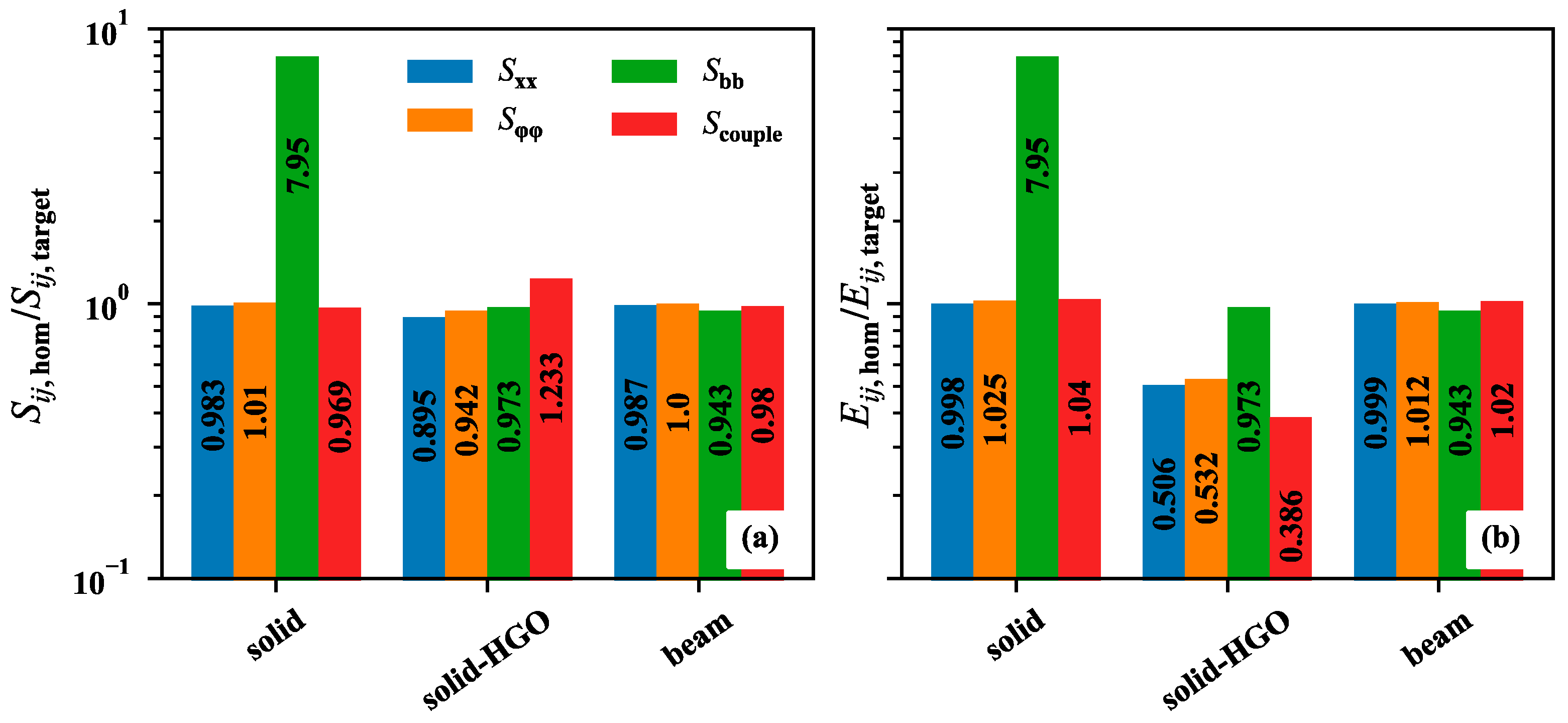
Three efficient cable-modeling approaches that can account for the tension/torsion coupling are investigated, and their and components are plotted in Figure 9. Similar to the cubic approaches, the bending stiffness of the solid approach is too high by a factor of 7.8. The solid, solid–HGO, and beam approaches can capture well; see Figure 9a. The largest differences are observed for in the solid–HGO approach, which is 22% higher than the target value. Note that due to having only three calibration parameters in the HGO approach, the four independent stiffness parameters cannot all be fitted at the same time. Other HGO parameters such as D, , and could be fitted as well but do not help to improve the accuracy of .
The components of the matrix of the solid and the beam approach in Figure 9b fit well to the target components, except for the of the linear elastic solid approach. For the solid–HGO approach, only the component fits well, whereas the other terms are lower by 46% to 60%. This is due to an amplification of the deviation of the components since the matrix is inverted to calculate . Furthermore, the convergence in the simulations with the solid HGO approach is bad, which requires many more iterations in the FEM simulation. The solid approach can therefore be used for applications where bending does not play a role, and the beam approach can be used in all cases where inaccuracies related to the coupling of the beam nodes to the rubber are acceptable—for example, because the rubber/cable interface is not of special interest in the model.
3.3. Three-Cable Models
The three-cable shear specimens of the szs-type with efficiently modeled cables are now evaluated in terms of stiffness, deformation fields, and stress fields, and compared to the full-geometry results. The rubber between the outer and the central cable is sheared, and the forces in the cables causes them to rotate in opposite directions, which is only slightly hindered by the rubber.
3.3.1. Stiffness of the Three-Cable Specimens
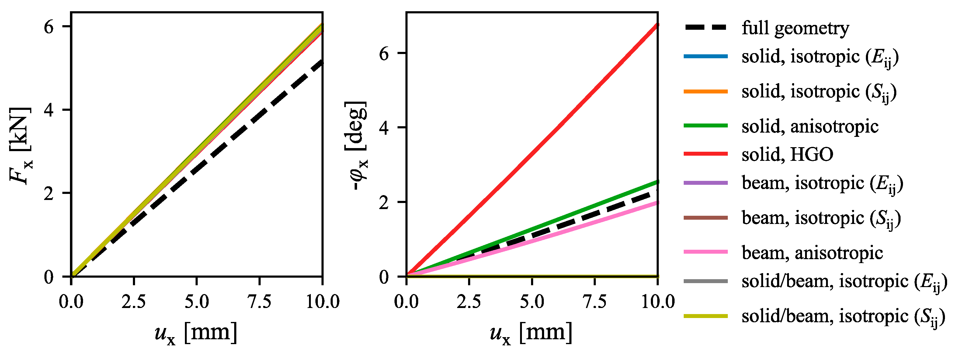
Figure 10 shows the longitudinal force and the end rotation of the central cable versus the end displacement . The dashed black line and the solid lines illustrate the response of the full-geometry and efficient approaches, respectively. A linear relation of both and with respect to can be seen.
There is good agreement between the curves of all the efficient cable-modeling approaches, but they all lie above the of the model with full geometry by about 14%. This can partly be explained by the non-uniform strain fields in the full-geometry model. Furthermore, the results in Section 3.1 show that the mesh of the full-geometry three-cable model can underestimate the cable stiffness by up to 4%, which can also contribute to this difference. In addition, the full-geometry model has a layer of rubber around the wires that can be sheared (see Figure 4, where the gap from the six outer wires to the surface of the whole cable can be written as r − − 2 − d = 0.3 mm). In the efficient models, this outer gap is assigned the same material properties as the rest of the cable, which is much stiffer than the rubber. When an efficient model is fitted to test data, the cable radius thus should be set to not include this layer of rubber to avoid this overestimation of stiffness in a rubber component. The end rotations of the central cable , plotted in Figure 10, are zero for all cubic modeling approaches since those models do not account for tension/torsion coupling. The anisotropic beam and anisotropic solid approaches show a good agreement with the full-geometry approach, whereas the solid–HGO approach overestimates the end rotation by about 150%.
The model size in terms of number of nodes, number of elements, degrees of freedom, necessary RAM to load the full stiffness matrix, and computation time are listed in Table 7 for all approaches in the three-cable model. There is a substantial difference in model size and computation time between the full-geometry approach and the efficient approaches, with the full-geometry model requiring about 50 GB of RAM to load the full stiffness matrix and a computation time of 4:35 h. The efficient three-cable models, on the other hand, need less than 2 GB of RAM and compute in about 2 min.
3.3.2. Deformations of the Three-Cable Specimens
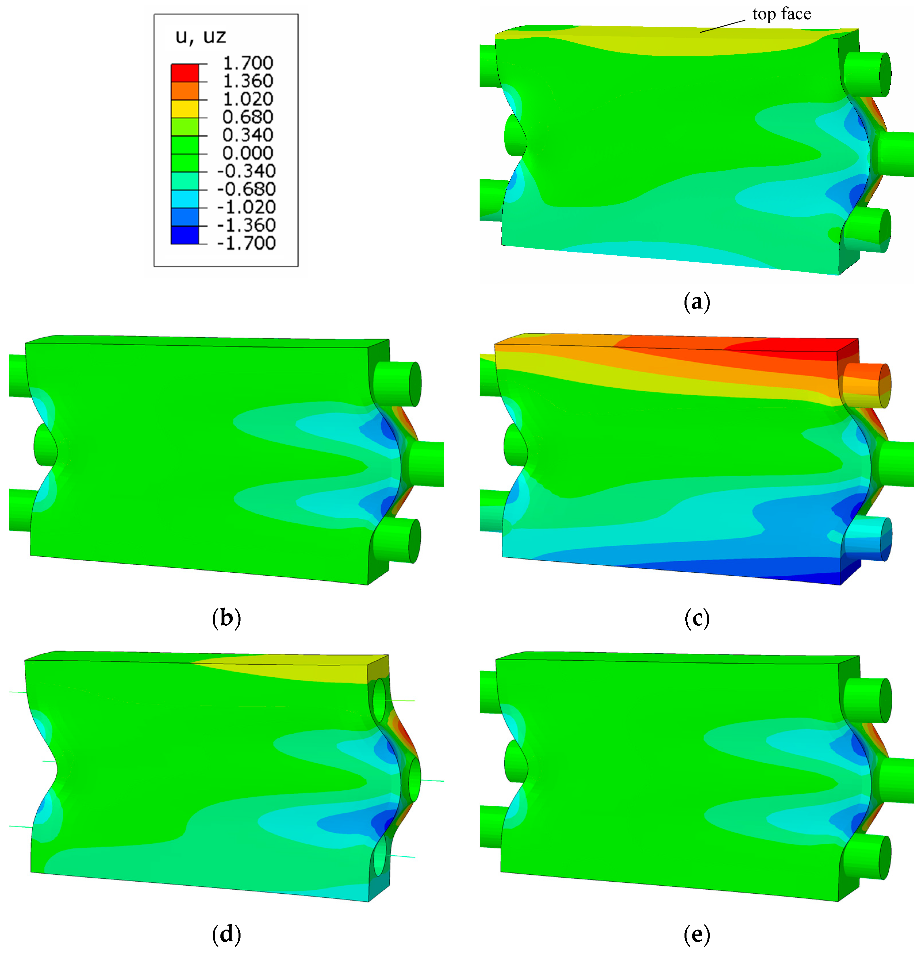
The tension/torsion coupling of the cables can cause a twisting of the specimen. One key result variable of this twist is the difference of the out-of-plane displacement , which is plotted in Figure 11. If is the same above and below the central cable, there is no twist—the displacement is merely a result of the Poisson effect in the rubber (especially the peaks at the right-hand side, which can be seen most clearly in Figure 11e). Otherwise, a twisting of the specimen occurs, which can be assessed by the displacement at the top and bottom surface. Since such behavior can only be described by the anisotropic cable-modeling approaches, only one of the cubic approaches (solid/beam, fitted to ) is shown for reference.
For the full-geometry model of Figure 11a, there is a distinct difference in the fields above and below the central cable: On the top and the bottom of the specimen, a of 0.7 mm and −0.7 mm is computed, respectively. Note that the highest values of at the top face occur at about 60% along the length of the rubber block in the specimen. The results for the cubic cable-modeling approach (see Figure 11e) show a completely symmetric field with respect to the xy-plane. The anisotropic solid approach in Figure 11b shows the same trend as the full-geometry model, but with a less pronounced twist of the specimen. The solid–HGO approach in Figure 11c, on the other hand, drastically overestimates the out-of-plane displacement of the specimen with on the top and bottom of the specimen of 1.7 mm and −1.7 mm, respectively. The best agreement with the full-geometry model is obtained by the anisotropic beam approach of Figure 11d: The fields are only slightly different above and below the center cable, with the top and bottom maximum values of occurring on the right end of the rubber block.
The poor performance of the HGO model can be explained by the unwanted coupling factors inherent to this approach. In addition, the HGO approach requires the highest computational effort for a convergence of the simulation. The better fit of the anisotropic beam approach compared to the anisotropic solid approach can only be attributed to their difference in bending stiffness: Since the twisting of the specimen is associated with a bending deformation of the cables, the excessive bending stiffness of the solid approach affects these results.
3.3.3. Stresses in the Three-Cable Specimens
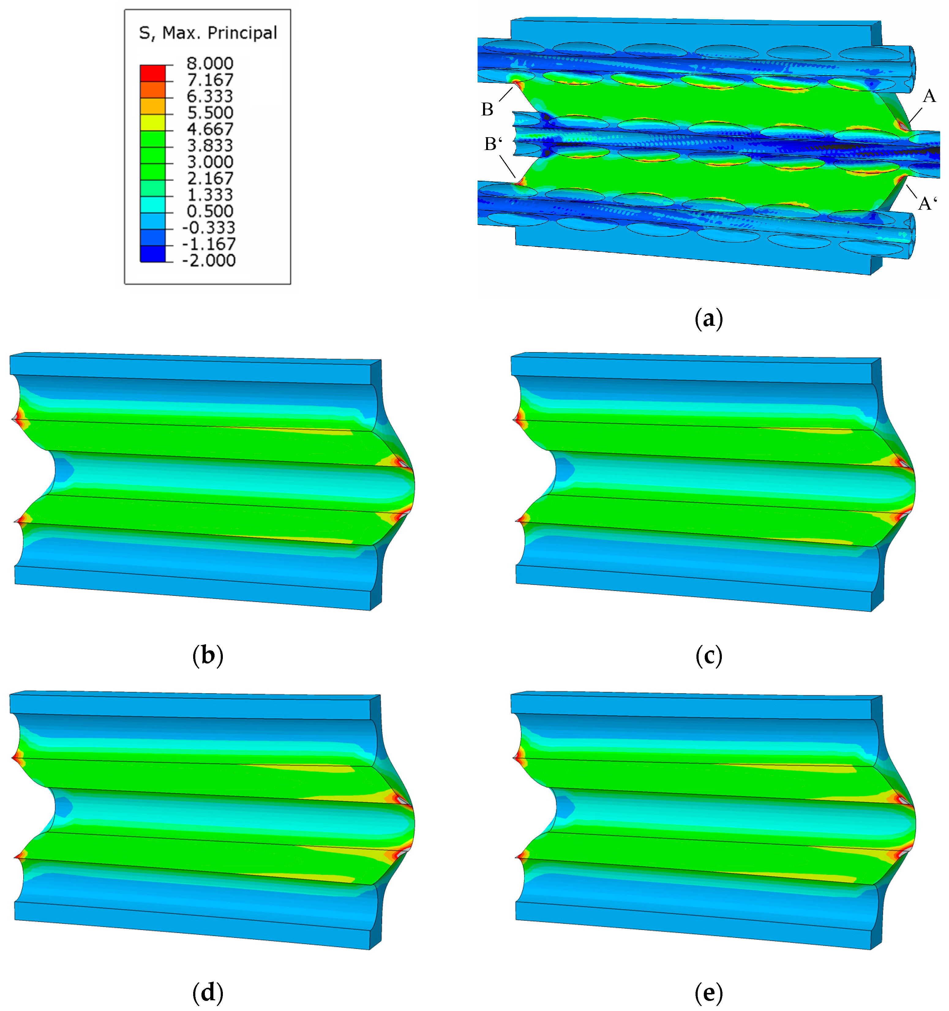
In many cases of reinforced rubber components, cable/rubber debonding and rubber failure is more relevant than deformations. Thus, the stresses in the rubber are evaluated in the following. It is assumed that the maximum principal stress is the best indicator for rubber failure. Figure 12 shows for the full-geometry model and various efficient modeling approaches. The specimen is cut in the plane of the cable axes. The main load of the rubber is shear between the central cable and the outer cables. These shear stresses, however, are not uniform and feature surface effects near the free surfaces at both ends of the rubber block (points A, A’, B, and B’): The highest occurs at the junction of the center cable and the rubber on the right-hand side of the specimen (point A and point A’). Those maximum values of amount to 12.54 MPa, 9.74 MPa, 9.87 MPa, 10.17 MPa, and 9.11 MPa for the full-geometry, solid–anisotropic, solid–HGO, beam–anisotropic, and solid/beam (fitted to ) approach, respectively. The junction of cable and rubber material imposes a singularity. This means that those stresses depend on the mesh size in the model, which must be accounted for in failure predictions. For relative comparisons like geometric studies with similar mesh, such results can be used nonetheless. There are also high stresses at the junction of the outer cables and the rubber on the left-hand side of the specimen (point B and point B’).
The stress field in the full-geometry model shown in Figure 12a shows additional peaks where the cable wires reach farthest into the space between the center cable and the outer cables. This effect introduces another parameter to the model: If such a region coincides with the surface of the rubber block (is close to point A or A’), the stresses will be considerably higher. This effect is not studied here but should be considered when predicting the failure of cable–rubber specimens.
The stress fields in the models with efficiently modeled cables are more uniform. The stresses generally increase towards the right side of the specimen. Similar to the full-geometry approach, the highest maximum principal stresses occur at points A and A’. The highest maximum principal stress in the solid/beam approach (see Figure 12e) of 9.11 MPa is lower than that of the other modeling approaches (9.87 MPa to 10.17 MPa). This can be explained by the very low Young‘s modulus of the solid elements in the solid/beam approach, which leads to a shear deformation between the beam and the cable surface. The differences in the highest computed of the varying cable-modeling approaches are rather low, indicating that for such three-cable specimens, a stress-based failure assessment is not sensitive to the selection of the modeling approach. There is a slight increase in the peaks due to the coupling term. For example, the beam approach computes maximum = 10.17 MPa in the anisotropic approach and 10.02 MPa in the cubic approach.
4. Conclusions
A variety of approaches for efficiently modeling the elastic response of a steel cable in a reinforced rubber component is introduced and evaluated both as a single cable and in a three-cable shear specimen. The aim is to reach an accurate representation of the high tensile stiffness, the high torsional stiffness, the low bending stiffness, and the tension/torsion coupling of steel cables. The modeling approaches considered consist of beam elements, solid elements, or a combination of both. In addition to an approach with linear elastic material behavior and cubic material symmetry, a special kind of anisotropic linear elastic material model is selected and fitted to capture the tension/torsion coupling. Furthermore, an approach using an anisotropic hyperelastic material model (HGO) is evaluated. The cable-modeling approaches are able to model the target stiffness of the cable to a varying extent:
- Solid linear elastic approaches: The bending stiffness is too high, but the other stiffness components are captured.
- Solid approach with anisotropic hyperelastic material: Only three parameters are available to fit four independent stiffness parameters. Not all four of them can be calibrated accurately at the same time. At least one of them differs up to 20% from the target value.
- Beam approach: All components of the target stiffness can be captured. However, the beam nodes are rigidly coupled to the rubber nodes at the cable surface, which is only valid if the cable is considerably stiffer than the rubber.
- Solid/beam approach: The tension/torsion coupling could be implemented in the beams, but the beam rotations would need to be coupled to the solid nodes. This coupling would induce numerical artifacts and is thus not implemented. Furthermore, the solid elements in the solid/beam approach have a very low Young‘s modulus that can lead to unphysical shear deformations inside the cable.
From those observations, the best modeling approach can be selected for a given application. The key questions for this selection is whether the cables experience a bending deformation and whether the tension/torsion coupling plays an important role in the model‘s application. Generally, the anisotropic beam approach is easy to calibrate and can capture the stiffness of the cable well. Inaccuracies introduced by the coupling of rubber nodes to the beam may not be acceptable, like in applications where evaluations at the rubber/cable interface require solid elements in the cable. In this case, the solid approach can be used if the cable bending is not relevant or the solid/beam approach if the tension/torsion coupling can be neglected. If both bending and tension/torsion coupling need to be captured, the HGO approach can be used, but it is associated with considerable discrepancies of all components of the stiffness matrix.
This work shows how to calculate and calibrate the geometric and material parameters of all cable modeling approaches and how to implement them. There is no approach that is suited for all possible applications, such as conveyor belts, hydraulic hoses, or tires. The modeling approach should be selected with care based on the type of loads the cables are exposed to in the application.
Author Contributions
Conceptualization, M.P., S.M.F. and C.S.; methodology, S.M.F. and M.P.; software, M.P.; validation, M.P.; formal analysis, M.P.; investigation, M.P. and S.M.F.; resources, M.P.; data curation, M.P.; writing—original draft preparation, M.P.; writing—review and editing, M.P., S.M.F. and C.S.; visualization, M.P.; supervision, C.S.; project administration, M.P.; funding acquisition, C.S. and M.P. All authors have read and agreed to the published version of the manuscript.
Funding
This research was supported by the Austrian Research Promotion Agency (FFG) within the BRIDGE framework as part of the project “Entwicklung einer Methodik zur Vorhersage des Versagens in elastomeren Gurten mittels Finite Elemente Simulation,” grant agreement.
Institutional Review Board Statement
Not applicable.
Informed Consent Statement
Not applicable.
Data Availability Statement
The methods for modeling cables are derived and evaluated independently of the FEM software used so other researchers can implement them into the FEM software they are using. Thus, no additional data need to be provided.
Conflicts of Interest
The authors declare no conflict of interest.
References
- Utting, W.S.; Jones, N. A Survey of Literature on the Behaviour of Wire Ropes. Wire Ind. 1984, 51, 623–629. [Google Scholar]
- Cardou, A.; Jolicoeur, C. Mechanical Models of Helical Strands. Appl. Mech. Rev. 1997, 50, 1–14. [Google Scholar] [CrossRef]
- Costello, G.A. Theory of Wire Rope; Mechanical Engineering Series; Springer: New York, NY, USA, 1997; ISBN 978-1-4612-7361-5. [Google Scholar]
- Feyrer, K. Wire Ropes Under Tensile Load. In Wire Ropes; Springer: Berlin/Heidelberg, Germany, 2015; pp. 59–177. ISBN 978-3-642-54995-3. [Google Scholar]
- Wang, X.-Y.; Meng, X.-B.; Wang, J.-X.; Sun, Y.-H.; Gao, K. Mathematical Modeling and Geometric Analysis for Wire Rope Strands. Appl. Math. Model. 2015, 39, 1019–1032. [Google Scholar] [CrossRef]
- Jiang, W.G.; Yao, M.S.; Walton, J.M. A Concise Finite Element Model for Simple Straight Wire Rope Strand. Int. J. Mech. Sci. 1999, 41, 143–161. [Google Scholar] [CrossRef]
- Foti, F.; de Luca di Roseto, A. Analytical and Finite Element Modelling of the Elastic–Plastic Behaviour of Metallic Strands under Axial–Torsional Loads. Int. J. Mech. Sci. 2016, 115–116, 202–214. [Google Scholar] [CrossRef] [Green Version]
- Chen, Y.; Meng, F.; Gong, X. Full Contact Analysis of Wire Rope Strand Subjected to Varying Loads Based on Semi-Analytical Method. Int. J. Solids Struct. 2017, 117, 51–66. [Google Scholar] [CrossRef]
- Cao, X.; Wu, W. The Establishment of a Mechanics Model of Multi-Strand Wire Rope Subjected to Bending Load with Finite Element Simulation and Experimental Verification. Int. J. Mech. Sci. 2018, 142–143, 289–303. [Google Scholar] [CrossRef]
- Utting, W.S.; Jones, N. The Response of Wire Rope Strands to Axial Tensile Loads—Part II. Comparison of Experimental Results and Theoretical Predictions. Int. J. Mech. Sci. 1987, 29, 621–636. [Google Scholar] [CrossRef]
- Chen, Z.; Yu, Y.; Wang, X.; Wu, X.; Liu, H. Experimental Research on Bending Performance of Structural Cable. Constr. Build. Mater. 2015, 96, 279–288. [Google Scholar] [CrossRef]
- Bonneric, M.; Aubin, V.; Durville, D. Finite Element Simulation of a Steel Cable-Rubber Composite under Bending Loading: Influence of Rubber Penetration on the Stress Distribution in Wires. Int. J. Solids Struct. 2019, 160, 158–167. [Google Scholar] [CrossRef] [Green Version]
- Frankl, S.; Pletz, M.; Schuecker, C. Incremental Finite Element Delamination Model for Fibre Pull-out Tests of Elastomer-Matrix Composites. Procedia Struct. Integr. 2019, 17, 51–57. [Google Scholar] [CrossRef]
- Nordell, L.K. Steel Cord Belt and Splice Construction. Bulk Solids Handl. 1993, 13, 685–693. [Google Scholar]
- Fedorko, G.; Molnar, V.; Dovica, M.; Toth, T.; Fabianova, J. Failure Analysis of Irreversible Changes in the Construction of the Damaged Rubber Hoses. Eng. Fail. Anal. 2015, 58, 31–43. [Google Scholar] [CrossRef]
- Frankl, S.M.; Pletz, M.; Wondracek, A.; Schuecker, C. Assessing Failure in Steel Cable-Reinforced Rubber Belts Using Multi-Scale FEM Modelling. J. Compos. Sci. 2022, 6, 34. [Google Scholar] [CrossRef]
- Nordell, L.; Qiu, X.; Sethi, V. Belt Conveyor Steel Cord Splice Analysis. Bulk Solids Handl. 1991, 11, 863–868. [Google Scholar]
- Abaqus. Dassault Systèmes; Simulia: Johnston, RI, USA, 2020. [Google Scholar]
- Cartraud, P.; Messager, T. Computational Homogenization of Periodic Beam-like Structures. Int. J. Solids Struct. 2006, 43, 686–696. [Google Scholar] [CrossRef] [Green Version]
- Holzapfel, G.A.; Gasser, T.C.; Ogden, R.W. A New Constitutive Framework for Arterial Wall Mechanics and a Comparative Study of Material Models. J. Elast. Phys. Sci. Solids 2000, 61, 1–48. [Google Scholar] [CrossRef]
- Gasser, T.C.; Ogden, R.W.; Holzapfel, G.A. Hyperelastic Modelling of Arterial Layers with Distributed Collagen Fibre Orientations. J. R. Soc. Interface 2006, 3, 15–35. [Google Scholar] [CrossRef] [PubMed]
- Froböse, T.; Overmeyer, L.; Poll, G. Verfahren zur Ermittlung der Materialparameter für die Auslegung von Stahlseil-Fördergurtverbindungen mit Hilfe der FEM; Berichte aus dem ITA; PZH Verlag: Garbsen, Germany, 2017; ISBN 978-3-95900-153-3. [Google Scholar]
- Gao, F.; Han, L. Implementing the Nelder-Mead Simplex Algorithm with Adaptive Parameters. Comput. Optim. Appl. 2012, 51, 259–277. [Google Scholar] [CrossRef]
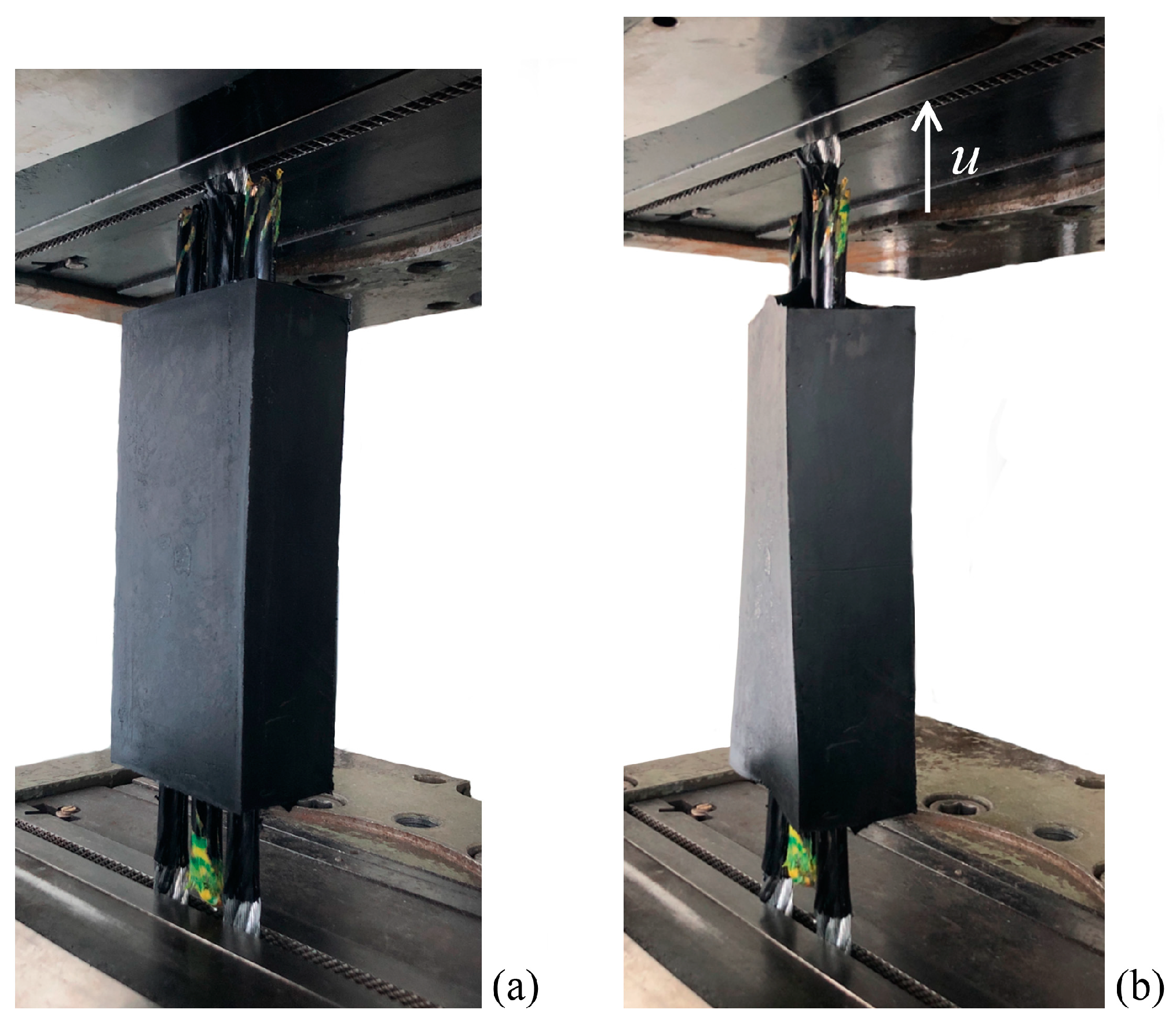
Figure 1.
A three-cable specimen: (a) unloaded and (b) vertically loaded with a twist due to a tension/torsion coupling of the cables.
Figure 1.
A three-cable specimen: (a) unloaded and (b) vertically loaded with a twist due to a tension/torsion coupling of the cables.

Figure 2.
Definition of the loads and strains of a cable.

Figure 3.
The three modeling approaches used for the cables: solid, beam, and a combination of both.
Figure 3.
The three modeling approaches used for the cables: solid, beam, and a combination of both.

Figure 4.
The geometry of the full-geometry single-cable model with its key parameters.

Figure 5.
The geometry of the three-cable specimen. Contact is defined in the orange-dashed regions.
Figure 5.
The geometry of the three-cable specimen. Contact is defined in the orange-dashed regions.

Figure 6.
Tensile force, torsional moment, and bending moment plotted over (a) the longitudinal strain and (b) the curvature of the seven-wire strand model for a mesh size of 0.5 mm and a relative cable length of 0.8.
Figure 6.
Tensile force, torsional moment, and bending moment plotted over (a) the longitudinal strain and (b) the curvature of the seven-wire strand model for a mesh size of 0.5 mm and a relative cable length of 0.8.

Figure 7.
Relative stiffness components of the strand model with (a) varied cable length using bilinear hexahedral elements with a mesh size of 0.5 mm and (b) varied mesh size with both bilinear hexahedral and quadratic tetrahedral elements for a relative cable length of 1.2.
Figure 7.
Relative stiffness components of the strand model with (a) varied cable length using bilinear hexahedral elements with a mesh size of 0.5 mm and (b) varied mesh size with both bilinear hexahedral and quadratic tetrahedral elements for a relative cable length of 1.2.

Figure 8.
Components of and relative to their target values for varying cable-modeling approaches without anisotropic material behavior. The parameters of the models are calibrated to (a,b) fit or (c,d) fit .
Figure 8.
Components of and relative to their target values for varying cable-modeling approaches without anisotropic material behavior. The parameters of the models are calibrated to (a,b) fit or (c,d) fit .

Figure 9.
The three anisotropic efficient cable-modeling approaches with their relative stiffness values in terms of (a) and (b) . Note that the parameters of the efficient models were calculated or fit to reach .
Figure 9.
The three anisotropic efficient cable-modeling approaches with their relative stiffness values in terms of (a) and (b) . Note that the parameters of the efficient models were calculated or fit to reach .

Figure 10.
Force–displacement and end rotation–displacement plots of the three-cable szs-type specimen with free end rotation .
Figure 10.
Force–displacement and end rotation–displacement plots of the three-cable szs-type specimen with free end rotation .

Figure 11.
Contour plots of the out-of-plane displacements in mm for (a) the full-geometry model and the four efficient cable-modeling approaches (b) solid, anisotropic, (c) solid, HGO, (d) beam, anisotropic, and (e) solid/beam, cubic (fit to Sij) of the three-cable szs-type specimen with free end rotation.

Figure 12.
Contour plots of the maximum principal stress (MPa) for (a) the full-geometry model and the four efficient cable-modeling approaches (b) solid, anisotropic, (c) solid, HGO, (d) beam, anisotropic, and (e) solid/beam, cubic (fit to Sij). The three-cable szs-type specimens are cut in the plane defined by z = 0.


Table 1.
Geometric parameters of the seven-wire strand.
| Parameter Name | Value |
|---|---|
| (mm) | 6 |
| (mm) | 1.95 |
| (mm) | 1.75 |
| (mm) | 0.25 |
| (°) | 11.8 |
Table 2.
Options of the efficient modeling approaches in terms of elements and material models used.
Table 2.
Options of the efficient modeling approaches in terms of elements and material models used.
| Linear Elastic | Hyperelastic | ||
|---|---|---|---|
| Approach | |||
| Solid | x | x | x |
| Beam | x | x | - |
| Solid/beam | x | - | - |
Table 3.
Geometry parameters of the three-cable model.
| Parameter Name | Value |
|---|---|
| (mm) | 100 |
| (mm) | 62 |
| (mm) | 20 |
| (mm) | 100 |
| (mm) | 10 |
| (mm) | 8 |
Table 4.
Information on the model size, necessary RAM to load the full stiffness matrix, and computation time (four cores of a six-core Intel Xeon E5-1650 v3 @ 3.5 GHz workstation with 128 GB RAM) for the full-geometry single-cable model (tensile load case) with varied element type, relative cable length, and mesh size.
| Mesh Type | Relative Length | Mesh Size (mm) | Nodes | Elements | Degrees of Freedom | Necessary RAM (MB) | Computation Time |
|---|---|---|---|---|---|---|---|
| Hex. | 0.2/2 | 0.5 | 14,427/158,021 | 10,162/109,965 | 40,397/396,291 | 240/3985 | 0:07 min/4:54 min |
| Hex. | 1.4 | 0.3/1.2 | 474,907/14,352 | 344,606/8744 | 1,203,365/35,068 | 19,867/205 | 20:19 min/0:08 min |
| Tet. | 1.4 | 0.75/2 | 40,509/36,660 | 26,702/14,304 | 100,875/82,882 | 738/442 | 4:56 min/0:43 min |
Table 5.
Stiffness parameters and from the full cable model with quadratic tetrahedral elements (mesh size of 0.75 mm) and cable length per strand length of 1.2.
Table 5.
Stiffness parameters and from the full cable model with quadratic tetrahedral elements (mesh size of 0.75 mm) and cable length per strand length of 1.2.
| 11,793 | kN | 7848 | kN | ||
| 15,594 | kN mm2 | 10,376 | kN mm2 | ||
| 7843 | kN mm | −15,601 | kN mm | ||
| 10,837 | kN mm2 | 10,837 | kN mm2 |
Table 6.
Material and geometry parameters for the efficient cable models from analytical calculation or calibration by FEM models.
Table 6.
Material and geometry parameters for the efficient cable models from analytical calculation or calibration by FEM models.
| Fit Towards | |||||
|---|---|---|---|---|---|
| Solid | 69.39 | 5.097 | - | ||
| 104.3 | 7.660 | 17.32 | |||
| Fit towards | * (GPa) | * (GPa) | k ** [1] | * (°) | |
| Solid, HGO | 0.7581 | 26.47 | 0.0 | 14.08 | |
| Fit towards | (GPa) | (GPa) | (mm) | * (MPa) | |
| Beam | 452.2 | 216.6 | 2.35 | - | |
| 1021 | 735.1 | 1.917 | 531.5 | ||
| Solid/beam | Fit towards | (GPa) | (GPa) | ** (mm) | (GPa) |
| 10.65 | 5.097 | 0.006 | 58,740,000 | ||
| 10.65 | 7.660 | 0.006 | 93,628,000 |
* Calibrated to fit . ** Chosen values.
Table 7.
Information on the model size, necessary RAM to load the full stiffness matrix, and computation time (four cores of a six-core Intel Xeon E5-1650 v3 @ 3.5 GHz workstation with 128 GB RAM) with varied model setup of the three-cable models.
Table 7.
Information on the model size, necessary RAM to load the full stiffness matrix, and computation time (four cores of a six-core Intel Xeon E5-1650 v3 @ 3.5 GHz workstation with 128 GB RAM) with varied model setup of the three-cable models.
| Nodes | Elements | Degrees of Freedom | Necessary RAM (MB) | Comp. Time | |
|---|---|---|---|---|---|
| Full geometry | 1,528,220 | 641,279 | 3,282,099 | 50,509 | 4:35 h |
| Solid | 165,198 | 77,642 | 338,343 | 1953 | 2:16 min |
| Beam | 74,053 | 33,990 | 165,081 | 843 | 0:46 min |
| Solid/beam | 166,056 | 78,071 | 393,630 | 1961 | 1:45 min |
Publisher’s Note: MDPI stays neutral with regard to jurisdictional claims in published maps and institutional affiliations. |
© 2022 by the authors. Licensee MDPI, Basel, Switzerland. This article is an open access article distributed under the terms and conditions of the Creative Commons Attribution (CC BY) license (https://creativecommons.org/licenses/by/4.0/).
Share and Cite
MDPI and ACS Style
Pletz, M.; Frankl, S.M.; Schuecker, C. Efficient Finite Element Modeling of Steel Cables in Reinforced Rubber. J. Compos. Sci. 2022, 6, 152. https://0-doi-org.brum.beds.ac.uk/10.3390/jcs6060152
AMA Style
Pletz M, Frankl SM, Schuecker C. Efficient Finite Element Modeling of Steel Cables in Reinforced Rubber. Journal of Composites Science. 2022; 6(6):152. https://0-doi-org.brum.beds.ac.uk/10.3390/jcs6060152
Chicago/Turabian StylePletz, Martin, Siegfried Martin Frankl, and Clara Schuecker. 2022. "Efficient Finite Element Modeling of Steel Cables in Reinforced Rubber" Journal of Composites Science 6, no. 6: 152. https://0-doi-org.brum.beds.ac.uk/10.3390/jcs6060152