A Practical Procedure for Predicting the Remaining Fatigue Life at an Arbitrary Stress Ratio

Abstract

A practical procedure for predicting the remaining fatigue life at an arbitrary stress ratio is developed and verified. The procedure was based on the validated damage function, in conjunction with the Kim and Zhang S-N curve model. The damage function was used for finding various iso-damage points dependent on three independent variables (i.e., stress level, number of fatigue cycles, and stress ratio). The verification was conducted using Alclad 24S-T aluminium alloy, available in the literature for fatigue loading varied under three different loading schemes. The first scheme was for two different stress ratios, the second was for three different stress ratios, and the last was for a single stress ratio as a special case. The prediction accuracies were found to be in an error range of −0.1 to 5.6%, −0.5 to −0.6, and 1.5 to 1.7% for the 1st, 2nd, and 3rd schemes, respectively.

1. Introduction

The term ‘fatigue’ in engineering seemingly first appeared in 1854 [1]. Fatigue is a phenomenon that takes place when the progressive damage under cyclic loading occurs to materials. There have been two different ways to approach the fatigue damage problems. One of the ways is to deal with cracks individually using fracture mechanics parameters, such as the stress intensity factor. The other way is to deal with “small” cracks [2] for fatigue life in a collective manner for crack initiation and growth at a relatively large scale, which requires an S-N curve model for characterisation (S and N in the acronym stand for stress and number of fatigue loading cycles, respectively).

Predicting the remaining fatigue life (RFL) following a prior fatigue loading associated with the S-N behaviour of the engineering materials has been a challenge since Palmgren [3] and Miner [4] attempted empirically. The history reveals that the application of the empirical approaches has been limited to some special cases, as reviewed in ref. [5]. Eskandari and Kim [5] eventually established a theoretical framework for fatigue damage validity, in conjunction with the Kim and Zhang S-N curve model [6,7]. The RFL depends on the fatigue damage accumulated during fatigue loading. The fatigue damage can be quantified using the damage function [5], which is, in general, a function of multiple independent variables. Quantified damage can be applicable to both composite and monolithic materials independent of the damage mechanism types involved [5]. If a material is subjected to a constant loading amplitude at a stress ratio (R), the RFL may be considered as a function of two variables, i.e., stress level and number of loading cycles. If a material is subjected to a different loading amplitude as a result of changing the stress ratio (R), it may be considered as a function of three variables, i.e., stress level, number of loading cycles, and R. In this case, it may need to have a predicted S-N curve to deal with a new stress ratio.

Kim and Huang [8] confirmed and verified a method for predicting the RFL with a new method for S-N curve characterisation applicable for time dependent materials, using the fatigue damage as a function of two independent variables at a single stress ratio (R) under tension-tension loading. As a natural progression, the prediction of the RFL using the fatigue damage as a function of three independent variables has been desired. This implies that, to find the parameters of the damage function, there must be a mathematical relationship between the stress ratio and S-N curve, given that the parameters of the damage function can be obtained from a relevant S-N curve. Kim [9,10] recently developed a practical method for predicting S-N curves at an arbitrary stress ratio, allowing us to proceed with further development of the three-variable problem. A solution to the three-variable problem may be important for potentially dealing with random fatigue loading in the future, given that the two variable approach is limited to a fixed stress ratio.

The purpose of the present paper was to develop a new procedure for predicting the RFL, using the fatigue damage function involving three independent variables. A successful outcome of the present work may be potentially a firm basis for developing a methodology for predicting the RFL under random fatigue loading.

2. The Theory

The Kim and Zhang S-N curve model has been evaluated [6,11,12] to be best suited not only for fatigue characterisation, but also for the prediction of the stress ratio (R = σ_min/σ_max = valley stress/peak stress) effect on the fatigue lives of composite materials. The number of cycles at failure (N = N_f) in the model with the lowest cycle (N = N₀) for material breaking point is given as a function of applied peak stress (σ_max), which is as follows:

$$N_f=\frac{{\left({\sigma }_{uT}\right)}^{-\beta }}{\alpha \left(\beta -1\right)}\left[{\left(\frac{{\sigma }_{max}}{{\sigma }_{uT}}\right)}^{1-\beta }-1\right]+N_0$$

(1)

or inversely,

$${\sigma }_{max}={\sigma }_{uT}{\left(\frac{\alpha \left(\beta -1\right)\left(N_f-N_0\right)}{{\left({\sigma }_{uT}\right)}^{-\beta }}+1\right)}^{\frac{1}{1-\beta }}$$

(2)

where $N_0$ = lowest number of cycles at the material breaking point,

• σ_uT = ultimate tensile strength, and
• α, β = damage parameters.

Although the value of $N_0$ is, in general, not exactly 0.5 for R ≠ 0 and R ≠ ±∞, it may be practically reasonable to approximate the cycle to be 0.5 cycle for an S-N curve characterisation. In fact, the breaking point is usually not obtainable from a fatigue testing machine because of the limited controllability, but it can be obtained from a universal testing machine. A practical method for using the value of 0.5 is proposed for time-dependent materials applicable to metallic materials [8].

The parameters (α, β) are obtained from the fatigue damage rate for T-T (tension-tension) loading or T-C (tension-compression) (if σ_uT > σ_uC (compressive strength)) and given by the following equation:

$$\frac{\partial D_f}{\partial N_f}=\alpha {\left({\sigma }_{max}\right)}^{\beta }$$

(3)

where D_f is the fatigue damage at tensile fatigue failure independent of stress ratio, which is defined by the following equation:

$$D_f=1-\frac{{\sigma }_{max}}{{\sigma }_{uT}}$$

(4)

A Matlab script for determining α and β is available in ref. [8]. The two parameters (α and β) in Equation (3) are determined by numerically differentiating an experimental fatigue data set for $\left(1-{\sigma }_{\max }/{\sigma }_{\mathrm{uT}}\right)$ versus N_f, followed by linearization by taking log on both sides of the differentiated data set. As a result, the intercept of the least square line of the differentiated data set becomes log α and β becomes its slope. If σ_uT < σ_uC for C-T (compression-tension) or C-C (compression-compression) loading, ${\sigma }_{uT}$ and ${\sigma }_{max}$ in Equations (1)–(4) are replaced with ${\sigma }_{uC}$ and ${\sigma }_{min}$, respectively [10].

The fatigue damage function (D) for any point on S-N plane given by the following equation [5,13]:

$$D=D_f{d}_f^n$$

(5)

where n is the validated exponent to be determined according to the practical procedure described in Appendix A, and $d_f$ is the (general) location factor with a value range of 0 to 1 for a point on the S-N plane at an arbitrary number of cycles (N) and peak stress (${\sigma }_{max}$), defined for a point b (Figure 1) as

$$d_f=\frac{\log N-\log N_0}{\log N_f-\log N_0}$$

(6)

3. Development of Procedure for Predicting the Remaining Fatigue Life at an Arbitrary R

The procedure to be developed here is based on the theory above. If the prediction of RFL is for a case of a single R, Equations (1)–(5) can be used for finding an iso-damage point at a new stress level on an S-N plane. If it is for a case of an arbitrary R at a new stress level, the same equations can be used but require another set of different parameter values from a new S-N curve. Thus, at least two S-N curves for a particular loading zone (e.g., T-T loading) in the CFL (constant fatigue life) diagram [10] are necessary for the latter case prediction. It should be noted that any other S-N curve can be predicted in each loading zone, provided that two S-N curves are available in the corresponding loading zone according to the method in ref. [10], allowing us to predict the RFL at a new stress level with any other R.

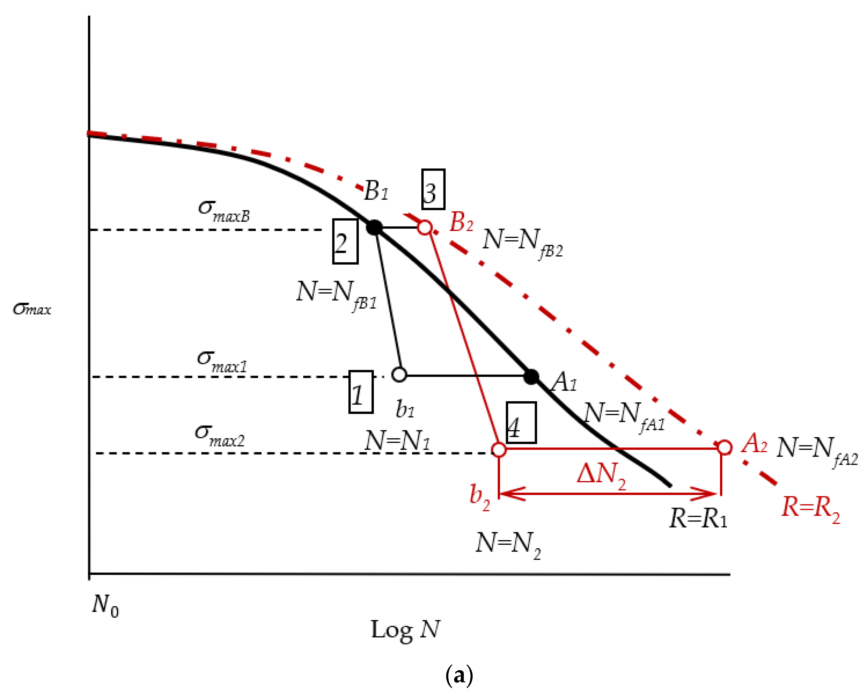
As schematically illustrated in Figure 1a, two S-N curves for two different stress ratios (i.e., R₁ and R₂) are considered here. When the fatigue load cycling at ${\sigma }_{max}={\sigma }_{max1}$ stops at a point b₁ under the S-N curve with R = R₁ and is then changed to ${\sigma }_{max}={\sigma }_{max2}$ with a different stress ratio R = R₂, a method for predicting the remaining fatigue life ($\mathsf{\Delta }{N}_2$) at R = R₂ may be developed. The sequence number given in each box (i.e., 1 to 4) in Figure 1a may be useful to indicate each point for sequential consideration. The following procedure involves mainly finding iso-damage points under two different S-N curves.

The location factor ($d_{fb1}$) at the first point b₁ (Figure 1a) with N = N₁ at ${\sigma }_{max}={\sigma }_{max1}={\sigma }_{maxA1}$ for R = R₁ is found according to Equation (6),

$$d_{fb1}=\frac{\log N_1-\log N_{01}}{\log N_{fA1}-\log N_{01}}$$

(7)

following the calculation of number of cycles at failure ($N_{fA1}$) at ${\sigma }_{max}={\sigma }_{maxA1}$ for R = R_1,

$$N_{fA1}=\frac{{\left({\sigma }_{uT}\right)}^{-{\beta }_1}}{{\alpha }_1\left({\beta }_1-1\right)}\left[{\left(\frac{{\sigma }_{maxA1}}{{\sigma }_{uT}}\right)}^{1-{\beta }_1}-1\right]+N_{01}$$

(8)

where each subscript ‘1’ indicates R = R₁.

The damage of the first iso-damage point ($D_{f{B}_1}$) at the 2nd point B₁, the damage of which is equal to that at the 1st point b₁ ($D_{f{b}_1}$), is required to be found with

$$D_{f{B}_1}\left(=D_{f{b}_1}\right)=D_{f{A}_1}{\left(d_{fb1}\right)}^{n_1}$$

(9)

using Equation (5). The second iso-damage point under R = R_2, damage ($D_{f{B}_2}$) at the 3rd point B₂ with R = R₂ is found at the same stress level on the S-N curve with R = R₂ according to Equation (4), giving the following equation:

$$D_{f{B}_2}=D_{f{A}_1}{\left(d_{fb1}\right)}^{n_1}$$

(10)

Thus, damage at the third iso-damage point b₂ ($D_{f{b}_2}$) at a new stress level ${\sigma }_{max2}$ is required to be found for R = R₂, the damage of which is equal to that of the 3rd point B₂ and to that of the point b₁ so that

$$D_{f{b}_2}\left(=D_{f{B}_2}\right)=D_{f{A}_2}{\left(d_{fb2}\right)}^{n_2}$$

(11)

Accordingly, the location factor for the point b₂ is found from Equations (9)–(11).

$$d_{fb2}={\left(\frac{D_{f{B}_2}}{D_{f{A}_2}}\right)}^{1/n_2}$$

(12)

and thus, the remaining fatigue life ($\mathsf{\Delta }{N}_2$) for R = R₂ is predicted to be

$$\mathsf{\Delta }{N}_2=N_{f{A}_2}-N_2$$

(13)

The practical sequence of the calculations with details involving two stress ratios is provided in

Table 1. Sequence of calculations for predicting the remaining fatigue life in volving two stress ratios.

Steps	Equations for Calculation	Comments
1	$N_{fA1}=\frac{{\left({\sigma }_{uT}\right)}^{-{\beta }_1}}{{\alpha }_1\left({\beta }_1-1\right)}\left[{\left(\frac{{\sigma }_{max{A}_1}}{{\sigma }_{uT}}\right)}^{1-{\beta }_1}-1\right]+N_{01}$	Number of cycles at failure at ${\sigma }_{max}={\sigma }_{maxA1}$ for R = R1
2	$d_{fb1}=\frac{\log N_1-\log N_{01}}{\log N_{f{A}_1}-\log N_{01}}$	Location factor at point b1 at ${\sigma }_{max}={\sigma }_{maxA1}$ for R = R1
3	$D_{f{A}_1}=1-\frac{{\sigma }_{max{A}_1}}{{\sigma }_{uT}}$	Damage at failure at ${\sigma }_{max}={\sigma }_{maxA1}$ for R = R1
4	$D_{f{B}_1}={\left(d_{fb1}\right)}^{n_1}{D}_{f{A}_1}$	Damage at point B1 or B2 for R = R1 or R = R2
5	${\sigma }_{maxB}={\sigma }_{uT}\left[1-{\left(d_{fb1}\right)}^{n_1}{D}_{f{A}_1}\right]$	Stress at ${\sigma }_{max}={\sigma }_{maxB}$
6	$N_{fB1}=\frac{{\left({\sigma }_{uT}\right)}^{-{\beta }_1}}{{\alpha }_1\left({\beta }_1-1\right)}\left[{\left(\frac{{\sigma }_{maxB}}{{\sigma }_{uT}}\right)}^{1-{\beta }_1}-1\right]+N_{01}$	Number of cycles at failure at ${\sigma }_{max}={\sigma }_{maxB}$ for R = R1
7	$N_{fB2}=\frac{{\left({\sigma }_{uT}\right)}^{-{\beta }_2}}{{\alpha }_2\left({\beta }_2-1\right)}\left[{\left(\frac{{\sigma }_{maxB}}{{\sigma }_{uT}}\right)}^{1-{\beta }_1}-1\right]+N_{02}$	Number of cycles at failure at ${\sigma }_{max}={\sigma }_{maxB}$ for R = R2
8	$D_{f{B}_2}=1-\frac{{\sigma }_{maxB}}{{\sigma }_{uT}}$	Damage at failure at ${\sigma }_{max}={\sigma }_{maxB}$ for R = R2
9	$D_{f{A}_2}=1-\frac{{\sigma }_{maxA2}}{{\sigma }_{uT}}$	Damage at failure at ${\sigma }_{max}={\sigma }_{maxA2}$ for R = R2
10	$d_{fb2}={\left(\frac{D_{f{B}_2}}{D_{fA2}}\right)}^{1/n_2}$	Location factor at point b2 at ${\sigma }_{max}={\sigma }_{maxA2}$ for R = R2
11	$N_{fA2}=\frac{{\left({\sigma }_{uT}\right)}^{-{\beta }_2}}{{\alpha }_2\left({\beta }_2-1\right)}\left[{\left(\frac{{\sigma }_{max{A}_2}}{{\sigma }_{uT}}\right)}^{1-{\beta }_2}-1\right]+N_{02}$	Number of cycles at failure at ${\sigma }_{max}={\sigma }_{maxA2}$ for R = R2
12	$\log N_2=d_{fb2}\left(\log N_{f{A}_2}-\log N_{02}\right)-\log N_{02}$	Number of cycles (N2) at point b2 for R = R2
13	$\Delta N_2=N_{f{A}_2}-N_2$	Predicted remaining number of cycles at ${\sigma }_{max}={\sigma }_{maxA2}$ for R = R2

. If three or more different stress ratios are involved for various load variations, the same procedure developed here can be used for predicting RFLs by choosing progressively two S-N curves with the associated calculations.

The accuracy of the prediction is a measure of how closely the experimental failure points ($N_2+\mathsf{\Delta }{N}_2$) are located to the relevant S-N curve. The location of each experimental failure point can be determined from $\log \left({10}^{\log N_2}+\mathsf{\Delta }{N}_2\right)$ using Step 12 in Table 1. Accordingly, the accuracy may be calculated using an error calculation, which is as follows:

$$\mathrm{Error}=\frac{\log \left({10}^{\log N_2}+\mathsf{\Delta }{N}_2\right)-\log \left(N_{fA2}\right)}{\log (N_{fA2})-\log \left(N_0\right)}$$

(14)

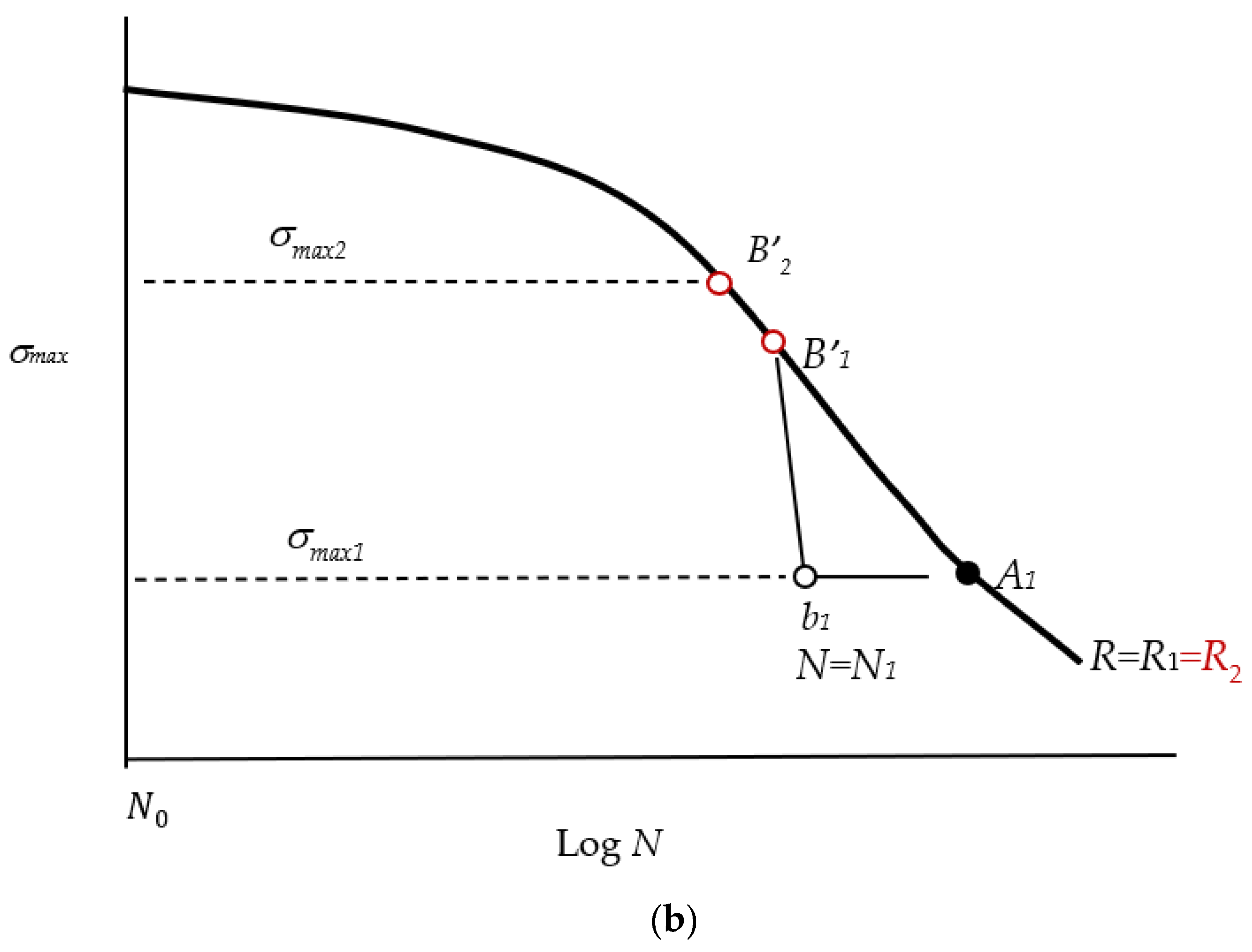
The procedure developed here is applicable for a special case of single R (i.e., R = R₁ = R₂). However, when low-high loading is applied with a single R, or with two stress ratios for similar S-N curves, an exceptional case is possible. Figure 1b is an example of a single R, where cyclic loading stopped at point b₁ at ${\sigma }_{max1}$ and increased to ${\sigma }_{max2}$ for further loading but it is possible that the new stress level of the iso-damage found at point B’₁ on the S-N curve is lower than that of point B’₂ on the S-N curve at the 2nd stress (σ_max2), when experimental/numerical uncertainties are high. In this case, the failure point may be approximated to be N_fB’2 + ΔN₂ using Equation (1) and an experimental value of ΔN₂, given that the damage values at two points B’₁ and B’₂ are usually not much different. Therefore, an error of RFL prediction may be as follows,

$$\mathrm{Error}=\frac{\log \left({10}^{\log N_{B^{\prime }2}}+\Delta N_2\right)-\log \left(N_{f{B}^{\prime }2}\right)}{\log (N_{f{B}^{\prime }2})-\log \left(N_0\right)}$$

(15)

4. Experimental Data

Fatigue experimental data sets for Alclad 24S-T aluminium alloy with an ultimate strength of 475 MPa were obtained from ref. [4] for three different stress ratios, R = −0.2, 0.2, and 0.5 (Figure 2). They were fitted to Equation (1) with the following parameter values: α = 1.65$\times$10⁻¹⁶, β = 4.197, and $N_0$ = 0.5 for R = −0.2; α = 6.47$\times$10⁻¹³, β = 2.582, and $N_0$ = 0.5 for R = 0.2; and α = 9.37$\times$10⁻¹⁶, β = 3.538, and $N_0$ = 0.5 for R = 0.2. The dashed lines of each S-N curve represent a confidence interval of 95%. The confidence interval for R = 0.5 appears to be relatively large, due to the small number of data points. The test specimens for the data sets were of dog-bone-shape made from flat sheet with material grain orientation perpendicular to sinusoidal fatigue loading.

The results of the RFL experiments for ΔN₂ conducted for the material used for the S-N behaviours shown in Figure 2 were also obtained from ref. [4] and are listed in

Table 2. Loading schemes and RFL experimental results (ΔN₂) with prediction errors.

R	(MPa)	$\times$1000 Cycles	logNf from Equation (1)	Predicted b2 (log N2)	Error of RFL Prediction
−0.2	σmax1 = 241	N1 = 40	NfA1 = 4.930	-
0.2	σmax2 = 224	ΔN2 = 149.5	NfA2 = 5.438	5.107	−0.1%
−0.2	σmax1 = 259	N1 = 40	NfA1 = 4.820	-
0.2	σmax2 = 172	ΔN2 = 423	NfA2 = 5.679	5.271	−1.8%
−0.2	σmax1 = 276	N1 = 30	NfA1 = 4.713	-
0.2	σmax2 = 184	ΔN2 = 83	NfA2 = 5.622	5.172	4.3%
−0.2	σmax1 = 276	N1 = 35	NfA1 = 4.713	-
0.2	σmax2 = 184	ΔN2 = 32.5	NfA2 = 5.622	5.233	5.3%
0.2	σmax1 = 172	N1 = 312	NfA1 = 5.679	-
−0.2	σmax2 = 259	ΔN2 = 56.8	NfA2 = 4.820	4.849	−5.6%
0.2	σmax1 = 184	N1 = 200	NfA1 = 5.622	-
−0.2	σmax2 = 276	ΔN2 = 46.2	NfA2 = 4.713	4.620	−4.6%
0.2	σmax1 = 172	N1 = 350	NfA1 = 5.679	-
−0.2	σmax2 = 259	ΔN2 = 23.8	NfA2 = 4.820	4.904	− 3.8%
−0.2	σmax1 = 276	N1 = 20	NfA1 = 4.713	-
0.2	σmax2 = 276	ΔN2 = 50	NfA2 = 5.215	4.850	-
0.2	σmax1 = 276	N1 = 70.334 + 50	NfA1 = 5.215	-
0.5	σmax2 = 276	ΔN2 = 143	NfA2 = 5.628	5.490	−0.5%
−0.2	σmax1 = 207	N1 = 40	NfA1 = 5.165
0.2	σmax2 = 224	ΔN2 = 80	NfA2 = 5.438	4.999
0.2	σmax1 = 224	N1 = 98.937 + 80	NfA1 = 5.438
0.5	σmax2 = 276	ΔN2 = 80	NfA2 = 5.628	5.583	− 0.6%
−0.2	σmax1 = 241	N1 = 33	Nf1 = 4.930
−0.2	σmax2 = 190	ΔN2 = 108.7	Nf1 = 5.294	4.718	1.7%
−0.2	σmax1 = 190	N1 = 127	Nf1 = 5.294
−0.2	σmax2 = 276	ΔN2 = 6.3	Nf1 = 4.713	N/A	1.5%

. The data in Table 2 consist of three load schemes for experimental variation, i.e., the first scheme is for two different stress ratios (i.e., R = −0.2 and 0.2), the second scheme for three different stress ratios (i.e., R = −0.2, 0.2, and 0.5), and the last scheme for a single stress ratio (i.e., R = −0.2). The first part of the first load scheme is for high-low loading. For example, the first applied maximum fatigue stress at σ_max1 = 241 MPa was stopped at N = 40,000 cycles with R = −0.2, followed by a decrease to σ_max2 = 224 MPa with R = 0.2, resulting in specimen failure in 149,500 cycles (=ΔN₂). The second part of the first load scheme was for low-high loading (e.g., σ_max = 172 to 259 MPa).

The second load scheme was for three stress ratios, i.e., R = −0.2, R = 0.2 and R = 0.5 (Table 2). In the first part of this load scheme, for example, the first fatigue loading at σ_max1 = 276 MPa with R = −0.2 was stopped at N = 20,000 cycles, followed by the same stress σ_max2 = 276 MPa, but with a different stress ratio R = 0.2 for further loading ΔN₂ = 50,000 cycles without failure at this point. This experiment continued at the same stress but with a different stress ratio, R = 0.5, until the specimen broke due to additional cycling ΔN₂ = 143,000 cycles.

The last load scheme was for a special case with a single stress ratio for both high-low and low high loadings.

5. Results and Discussion

The experimental failure points (represented by square and circular symbols) obtained from cyclic loading, which varied from R = −0.2 to 0.2, are shown in Figure 3a,b, with reference to the relevant S-N curves selected from Figure 2. Two different ways of loading, i.e., high-low and low-high loadings, are separately given in Figure 3a,b respectively. The straight lines, as already described in Section 3, represent the applied loading paths and connections between iso-damage points. The three iso-damage points were calculated according to the procedure developed earlier, in conjunction with experimental data points and numerically calculated values for exponent (n) in Equation (5) (i.e., n = 7.47, 9.38, 9.69 for R = −0.2, 0.2, and 0.5, respectively). The error of RFL prediction according to Equation (14) was found to be in a range of −0.1 to 5.3%, as listed in Table 2 for high-low loading (Figure 3a) and was found to be in a range of −5.6 to −3.8% (Figure 3b) for low-high loading.

Figure 3c shows two experimental failure points represented by circular symbols (it looks as though they are one because two points are almost identical). This is a case where three stress ratios (i.e., R = −0.2, 0.2, 0.5) are involved in load variations. Note that the specimen failure did not occur at the 2nd R (=0.2) for the 1st additional cyclic loading ($\mathsf{\Delta }{N}_2$), but took place at the 3rd R (=0.5), due to the 2nd additional cyclic loading ($\mathsf{\Delta }{N}_2$). The first load variation was conducted with a constant σ_max (=276 MPa), while the second load variation was with different stress levels (σ_max = 207, 224, and 276 MPa). Equation (14) was used again for prediction accuracy to find how the failure point is close to the S-N curve with R = 0.5. The prediction errors were found to be −0.5% and −0.6% for the 1st (σ_max = constant = 276 MPa) and 2nd (σ_max = 207, 224, 276 MPa) load variations, respectively. They appear to be more accurate than those of the first load scheme (Figure 3a,b).

Figure 3d shows a special case where a single S-N curve for R = −0.2 is used. Two failure points are shown from two different ways of load variation. One is represented by a square symbol for high-low loading and its prediction error was found to be 1.7%, according to Equation (14). The other is represented by a circular symbol for low-high loading. This is an exceptional case where the iso-damage point on S-N curve at the stress level (σ_max = 255 MPa), whose damage is equal to that of the load stopping point, does not correspond to that the new stress level (σ_max = 276 MPa) applied for load variation. In this case, as already discussed in Section 3, Equation (15) may be used for a prediction accuracy and an error of 1.5% was found.

When all the failure points are considered, no noticeable trend affected by the load sequence is found in Figure 3. One might expect the load sequence effect to occur when the cyclic loading is varied. For example, when a stress level decreases to a lower stress level (i.e., high-low loading), the fatigue life may be expected to increase due to the crack closure [14], or vice versa. The scatters of data points in individual cases in Figure 3a,b, however, both display that the deviations of failure points from each S-N curve tend to be opposite to such an expectation, and that the predictions in Figure 3c,d are accurate without much deviation. Therefore, it may be deduced that the small cracks constituting the S-N curve behaviour are unlikely to be affected by the load sequence, unlike the long cracks. The behaviour observed here appears consistent with the other experimental results in the literature [8], even though some experimental uncertainties are always possible for different loading schemes.

6. Conclusions

A procedure for predicting the remaining fatigue life (RFL) associated with S-N curves and multiple stress ratios has been developed for engineering materials. It has been verified using experimental results obtained from three different loading schemes for an aluminium alloy. The first scheme was for two different stress ratios, the second was for three different stress ratios, and the last was for a single stress ratio as a special case. The prediction errors have been found to be in the range of −0.1 to 5.6%, −0.5 to −0.6, and 1.5 to 1.7% for the 1st, 2nd, and 3rd schemes, respectively.

References

- Braithwaite, F. On the fatigue and consequent fracture of metals. In Minutes of the Proceedings of Civil Engineers; ICE Publishing: London, UK, 1854; Volume 13, pp. 463–467. [Google Scholar] [CrossRef]
- Kitagawa, H.; Takashima, S. Application of Fracture Mechanics to Very Small Fatigue Cracks or the Cracks in the Early Stage. In Proceedings of the Second International Conference on Mechanical Behavior of Materials, American Society for Metals, Materials Park, OH, USA, 16–20 August, 1976; pp. 627–631. [Google Scholar]
- Palmgren, A.G. Die Lebensdauer von Kugellagern (Life Length of Roller Bearings in German). Z. Des Ver. Dtsch. Ing. 1924, 68, 339–341. [Google Scholar]
- Miner, M.A. Cumulative damage in fatigue. J. Appl. Mech. 1945, 67, 159–164. [Google Scholar] [CrossRef]
- Eskandari, H.; Kim, H.S. A Theory for mathematical framework and fatigue damage function for the S-N plane. In Fatigue and Fracture Test Planning, Test Data Acquisitions, and Analysis; ASTM STP1598; Wei, Z., Nikbin, K., McKeighan, P.C., Harlow, D.G., Eds.; ASTM International: West Conshohocken, PA, USA, 2017; pp. 299–336. [Google Scholar]
- Kim, H.S.; Zhang, J. Fatigue Damage and Life Prediction of Glass/Vinyl Ester Composites. J. Reinf. Plast. Compos. 2001, 20, 834–848. [Google Scholar] [CrossRef]
- Kim, H.S. Mechanics of Solids and Fracture, 4th ed.; Mechanics of Solids and Fracture (bookboon.com); Bookboon, Ventus Publishing ApS: London, UK, 2022. [Google Scholar]
- Kim, H.S.; Huang, S. S-N curve Characterisation for Composite Materials and Prediction of Remaining Fatigue Life Using Damage Function. J. Compos. Sci. 2021, 5, 76. [Google Scholar] [CrossRef]
- Kim, H.S. Prediction of S-N curves at various stress ratios for structural materials. Procedia Struct. Integr. 2019, 19, 472–481. [Google Scholar] [CrossRef]
- Kim, H.S. Theory and practical procedure for Predicting S-N curves at various stress ratios. J. Compos. Biodegrad. Polym. 2019, 2, 57–72. [Google Scholar] [CrossRef]
- Burhan, I.; Kim, H.S. S-N Curve Models for Composite Materials Characterisation: An Evaluative Review. J. Compos. Sci. 2018, 2, 38. [Google Scholar] [CrossRef]
- Burhan, I.; Kim, H.S.; Thomas, S. A refined S-N curve model. In Proceedings of the International Conference on Sustainable Energy, Environment and Information (SEEIE 2016), Bangkok, Thailand, 20–21 March 2016; AMSME-E107, 23/34-35 Traimit Road: Taladnoy, Bangkok, Thailand. pp. 412–416. [Google Scholar] [CrossRef]
- Kim, H.S. S–N curve and fatigue damage for practicality. In Creep and Fatigue in Polymer Matrix Composites, Woodhead Publishing Series in Composites Science and Engineering, 2nd ed.; Guedes, R.M., Ed.; Elsevier: Cambridge, MA, USA, 2019; pp. 439–463. [Google Scholar] [CrossRef]
- Elber, W. The significance of fatigue crack closure. In Damage Tolerance in Aircraft Structures, ASTM STP486; ASTM International: West Conshohocken, PA, USA, 1971; pp. 230–242. [Google Scholar]
Figure 1.
Loading schemes: (a) two S-N curves for the general case for changing stress from σmax1 with R = R1 to σmax2 with R = R2; and (b) a single S-N curve as a special case for an exception, where the iso-damage point does not correspond to that at the new stress level σmax2 when low-high loading is applied.
Figure 2.
Experimental fatigue data and Kim and Zhang S-N curved model fitted.
Figure 3.
Fatigue loading schemes and failure points: (a) high-low loading for R = −0.2 and R = 0.2; (b) low-high loading for R = −0.2 and R = 0.2; (c) loading for R = −0.2, 0.2 and 0.5; and (d) high-low and low-high loadings for a single stress ratio R = −0.2.