
Property Checking with Interpretable Error Characterization for Recurrent Neural Networks


Facultad de Ingeniería, Universidad ORT Uruguay, 11100 Montevideo, Uruguay
*
Authors to whom correspondence should be addressed.
†
Equal contribution.
Mach. Learn. Knowl. Extr. 2021, 3(1), 205-227; https://0-doi-org.brum.beds.ac.uk/10.3390/make3010010
Submission received: 16 December 2020
/
Revised: 25 January 2021
/
Accepted: 3 February 2021
/
Published: 12 February 2021
(This article belongs to the Special Issue Selected Papers from CD-MAKE 2020 and ARES 2020)
Abstract
:This paper presents a novel on-the-fly, black-box, property-checking through learning approach as a means for verifying requirements of recurrent neural networks (RNN) in the context of sequence classification. Our technique steps on a tool for learning probably approximately correct (PAC) deterministic finite automata (DFA). The sequence classifier inside the black-box consists of a Boolean combination of several components, including the RNN under analysis together with requirements to be checked, possibly modeled as RNN themselves. On one hand, if the output of the algorithm is an empty DFA, there is a proven upper bound (as a function of the algorithm parameters) on the probability of the language of the black-box to be nonempty. This implies the property probably holds on the RNN with probabilistic guarantees. On the other, if the DFA is nonempty, it is certain that the language of the black-box is nonempty. This entails the RNN does not satisfy the requirement for sure. In this case, the output automaton serves as an explicit and interpretable characterization of the error. Our approach does not rely on a specific property specification formalism and is capable of handling nonregular languages as well. Besides, it neither explicitly builds individual representations of any of the components of the black-box nor resorts to any external decision procedure for verification. This paper also improves previous theoretical results regarding the probabilistic guarantees of the underlying learning algorithm.
1. Introduction
Artificial intelligence (AI) is a flourishing research area with numerous real-life applications. Intelligent software is developed in order to automate processes, classify images, translate text, drive vehicles, make medical diagnoses, and support basic scientific research. The design and development of this kind of systems is guided by quality attributes that are not exactly the same as those that drive the construction of a typical software system. Indeed, a salient one is the degree to which a human being (e.g., a physician) can really understand the actual cause of a decision made by an AI system (e.g., the diagnostic of a disease). Such attribute is called interpretability [1,2,3].
Undoubtedly, artificial neural networks (ANN) are currently the cutting-edge AI models [4]. However, their inherent nature undermines human capability of achieving acceptable comprehension of the reasons of their outputs. A major obstacle towards interpreting their behavior is their deep architectures with millions of neurons and connections. Such overwhelming complexity attempts against interpretability even if ANN structure used in a particular context is known (e.g., convolutional neural networks in computer vision or recurrent neural networks in language translation) and the mathematical principles on which they are grounded are understood [5].
Thoroughly interpreting the functioning of AI components is a must when they are used in the context of safety- and security-critical domains such as intelligent driving [6,7], intrusion, attack, and malware detection [8,9,10,11,12], human activity recognition [13], medical records analysis [14,15], and DNA promoter region recognition [16], which involve using deep recurrent neural networks (RNN) for modeling the behavior of the controlled, monitored, or analyzed systems or data. Moreover, it is paramount to verify their outputs with respect to the requirements they must fulfill to correctly perform the task they have been trained for. Whenever a network outcome does not satisfy a required property, it appears necessary to be able to adequately characterize and interpret the misbehavior, in order to be able to properly correct the fault, which may involve redesigning and retraining the network. Indeed, when it comes to interpreting the error of an RNN with respect to a given requirement, typically expressed as a property over sequences (i.e., a language in a formal sense) it is useful to do it through an operational and visual characterization, as a means for gaining insight into the set of incorrect RNN outputs (e.g., wrong classification of a human DNA region as a promoter) in reasonable time.
One way of checking language properties in the context of RNN devoted to sequence classification, consists in extracting an automaton, such as a deterministic finite automaton (DFA) from the network and resort to automata-theoretic tools to perform the verification task on the extracted automaton. That is, once the automaton is obtained, it can be model-checked against a desired property using an appropriate model-checker [17]. This approach can be implemented by resorting to white-box learning algorithms such as the ones proposed in [18,19,20]. However, RNN are more expressive than DFA [21]. Therefore, the language of the learned automaton is, in general, an approximation of the sequences classified as positive by the RNN. The cited procedures do not provide quantitative assessments on how precisely the extracted DFA characterizes the actual language of the RNN. Nonetheless, this issue is overcome by the black-box learning algorithm proposed in [22] which learns DFA which are probably correct approximations (PAC) [23] of the RNN. This means that the error between the outputs of the analyzed RNN and the extracted DFA can be bounded with a given confidence.
When applied in practice, this general approach has several important drawbacks. The first one is state explosion. That is, the DFA learned from the RNN may be too large to be explicitly constructed. Another important inconvenience is that when the model-checker fails to verify the property on the DFA, counterexamples found on the automaton are not necessarily real counterexamples of the RNN. Indeed, since the DFA is an approximation of the RNN, counterexamples found on the former could be false negatives. Last but not least, it has been advocated in [24] that there is also a need for property checking techniques that interact directly with the actual software that implements the network.
To cope with these issues, Reference [25] devised a technique based on the general concept of learning-based black-box checking (BBC) proposed in [26]. BBC is a refinement procedure where DFA are incrementally built by querying a black-box. At each iteration, these automata are checked against a requirement by means of a model-checker. The counterexamples, if any, found by the model-checker are validated on the black-box. If a false negative is detected, it is used to refine the automaton. A downside of BBC is that it requires (a) fixing a formalism for specifying the requirements, typically linear-time temporal logic, and (b) resorting to an external model-checker to verify the property. Moreover, the black-box is assumed to be some kind of finite-state machine.
Instead, the method proposed in [25] performs on-the-fly property checking during the learning phase, without using an external model-checker. Besides, the algorithm handles both the RNN and the property as black-boxes and it does not build, assume, or require them to expressed in any specific way. The approach devised in [25] focuses on checking language inclusion, that is, whether every sequence classified by the RNN belongs to the set of sequences defined by the property. This question can be answered by checking language emptiness: the requirement is satisfied if the intersection of the language of the RNN and the negation of the property is empty, otherwise it is not. Language emptiness is tackled in [25] by learning a probably approximately correct DFA. On one hand, if the learning algorithm returns an empty DFA, there is a proven upper bound on the probability of the language to be nonempty, and therefore of the RNN not satisfying the property. In other words, the property is probably true with probabilistic guarantees given in terms of the algorithm parameters. On the other, if the output is a nonempty DFA, the language is ensured to be nonempty. In this case, the property is certainly false. Besides, the output DFA is an interpretable characterization of the error.
The contribution of this paper is twofold. First, we revise and improve the theoretical results of [25]. We extend the approach to checking not only language inclusion but any verification problem which can be reduced to checking emptiness. Besides, we provide stronger results regarding the probabilistic guarantees of the procedure. Second, we apply the method to other use cases, including checking context-free properties and equivalence between RNN.
The structure of the paper is the following. Section 2 reviews probably approximately correct learning. Section 3 introduces on-the-fly black-box property-checking through learning. Section 4 revisits the framework proposed in [25] and shows the main theoretical results. These include improvements with respect to the previously known probabilistic guarantees of the underlying learning algorithm. Section 5 describes the experimental results obtained in a number of use cases from different application areas. Section 6 discusses related works. Section 7 presents the conclusions.
2. Probably Approximately Correct Learning
Let us first give some preliminary definitions. There is a universe of examples which is denoted . Given two subsets of examples , the difference is the set of such that , or equivalently, the set , where is the complement of X. Their symmetric difference, denoted , is defined as . Examples are assumed to be identically and independently distributed (i.i.d.) according to an unknown probability distribution over .
A concept C is a subset of . A concept class is a set of concepts. Given an unknown concept , the purpose of a learning algorithm is to output a hypothesis that approximates C, where , called hypothesis space, is a class of concepts possibly different from .
The prediction error of a hypothesis H with respect to the unknown concept C measured in terms of the probability distribution is the probability of an example , drawn from , to be in symmetric difference of C and H. Formally:
An oracle draws i.i.d examples from following , and associates the labels according to whether they belong to C. An example is labeled as positive if , otherwise it is labeled as negative. Repeated calls to are independent of each other.
A Probably Approximately Correct (PAC) learning algorithm [23,27,28] takes as input an approximation parameter , a confidence parameter , a target concept , an oracle , and a hypothesis space , and if it terminates, it outputs an which satisfies with confidence at least . Formally:
The output H of a PAC-learning algorithm is said to be an -approximation of C with confidence at least , or equivalently, an -approximation of C.
Typically, is indeed composed of a sampling procedure that draws an example and calls a membership query oracle to check whether . Besides and , a PAC-learning algorithm may be equipped with an equivalence query oracle . This oracle takes as input a hypothesis H and a sample size m and answers whether H is an -approximation of C by drawing a sample of size m using , i.e., , and checking whether for all , iff , or equivalently, .
We revisit here some useful results from [25].
Lemma 1.
Let and such that H is an -approximation of C. For any subset , we have that with confidence .
Proof.
For any subset , it holds that . It follows that implies . Now, for any satisfying , we have that . Hence, any sample drawn by that ensures with confidence also guarantees with confidence . ☐
Proposition 1.
Let and such that H is an -approximation of C. For any :
with confidence at least .
Proof.
From Lemma 1 because and are subsets of . ☐
3. Black-Box Property Checking
3.1. Post-Learning Verification
Given an unknown concept , and a known property to be checked on C, we want to answer whether holds, or equivalently . One way of doing it in a black-box setting consists in resorting to a model-checking approach. That is, first learn a hypothesis of C with a PAC-learning algorithm and then check whether H satisfies property P. We call this approach post-learning verification. In order to be feasible, there must be an effective procedure for checking .
Assume an algorithm for checking emptiness exists. Proposition 2 from [25], proves that whichever the outcome of the decision procedure for , the probability of the same result not being true for C is smaller than , with confidence at least .
Proposition 2.
Let and such that H is an -approximation of C. For any :
- 1.
- if then , and
- 2.
- if then ,
with confidence at least .
Proof.
- 1.
- If then . Thus, and from Proposition 1(3) it follows that , with confidence at least .
- 2.
- If , from Proposition 1(4) we have that , with confidence at least . ☐
When applied in practice, an important inconvenience of this approach is that whenever P is found by the model-checker not to hold on H, even if with small probability, counterexamples found on H may not be counterexamples in C. Therefore, whenever that happens, we would need to resort to to draw examples from and call to figure out whether they belong to C in order to trying finding a concrete counterexample in C.
From a computational perspective, in particular in the application scenario of verifying RNN, we should be aware that the learned hypothesis could be too large and that the running time of the learning algorithm adds up to the running time of the model-checker, thus making the overall procedure impractical.
Last but not least, this approach could only be applied for checking properties for which there exists a model-checking procedure in . In our context, it will prevent verifying nonregular properties.
3.2. On-the-Fly Property Checking through Learning
To overcome the aforementioned issues, rather than learning an -approximation of C, Ref. [25] proposed to use the PAC-learning algorithm to learn an -approximation of . This approach is called on-the-fly property checking through learning.
Indeed, this idea can be extended to cope with any verification problem which can be expressed as checking the emptiness of some concept , which in the simplest case is . In such context, we have the following, more general, result.
Proposition 3.
Let , and such that H is an -approximation of . Then:
- 1.
- if then , and
- 2.
- if then ,
with confidence at least .
Proof.
Straightforward since , with confidence at least , by the fact that H is an -approximation of . ☐
Proposition 3 proves that checking properties during the learning phase yields the same theoretical probabilistic assurance as doing it afterwards on the learned model of the target concept C. Nevertheless, from a practical point of view, on-the-fly property checking through learning has several interesting advantages over post-learning verification. First, no model of C is ever explicitly built which may result in a lower computational effort, both in terms of running time and memory. Therefore, this approach could be used in cases where it is computationally too expensive to construct a hypothesis for C. Second, there is no need to resort to external model-checkers. The approach may even be applied in contexts where such algorithms do not exist. Indeed, in contrast to post-learning verification, an interesting fact in on-the-fly checking is that in the case the PAC-learning algorithm outputs a nonempty hypothesis, it may actually happen that the oracle draws an example belonging to at some point during the execution, which constitutes a concrete, real evidence of not being empty with certainty.
4. On-the-Fly Property-Checking for RNN
In this section we further develop the general principle of on-the-fly property checking in the context of RNN. More precisely, the universe is the set of words over a set of symbols , the target concept inside the black-box is a language implemented as an RNN, and the hypothesis class is the set of regular languages or equivalently of deterministic finite automata (DFA).
4.1. Bounded-: An Algorithm for Learning DFA from RNN
DFA can be learned with [29], an iterative algorithm that incrementally constructs a DFA by calling oracles and . PAC-based satisfies the following property.
Property 1
(From [29]). (1) If terminates, it outputs an -approximation of the target language. (2) always terminates if the target language is regular.
may not terminate when used to learn DFA approximations of RNN because, in general, the latter are strictly more expressive than the former [21,30,31]. That is, there exists an RNN C for which there is no DFA A with the same language. Therefore, it may happen that at every iteration i of the algorithm, the call to for the i-th hypothesis fails, i.e., , where is the sample set drawn by . Hence, will never terminate for C.
To cope with this issue, Bounded- has been proposed in [22]. It bounds the number of iterations of by constraining the maximum number of states of the automaton to be learned and the maximum length of the words used to calling , which are typically used as parameters to determine the complexity of a PAC-learning algorithm [32]. For the sake of simplicity, we only consider here the bound n imposed on the number of states. This version of Bounded- is shown in Algorithm 1.
| Algorithm 1: Bounded- |
 |
Bounded- works as follows. Similarly to , the learner builds a table of observations, denoted , by interacting with the teacher. This table is used to keep track of which words are and are not accepted by the target language. is built iteratively by asking the teacher membership queries through . is a finite matrix . Its rows are split in two. The “upper” rows represent a prefix-closed set words and the “lower” rows correspond to the concatenation of the words in the upper part with every . Columns represent a suffix-closed set of words. Each cell represents the membership relationship, that is, . We denote the empty word and the value of the observation table at iteration i.
The algorithm starts by initializing (line 1) with a single upper row , a lower row for every , and a single column for the empty word , with values .
At each iteration , the algorithm makes closed (line 7) and consistent (line 10). is closed if, for every row in the bottom part of the table, there is an equal row in the top part. is consistent if for every pair of rows in the top part, for every , if then .
Once the table is closed and consistent, the algorithm proceeds to build the conjectured DFA (line 13) which accepting states correspond to the entries of such that .
Then, Bounded- calls (line 14) to check whether is PAC-equivalent to the target language. For doing this, draws a sample of size defined as follows [29]:
If , the equivalence test succeeds and Bounded- terminates producing the output DFA . Clearly, in this case, we conclude that is an -approximation of the black-box.
Corollary 1.
For any , if Bounded- terminates with a DFA A which passes , then A is an -approximation of C.
Proof.
Straightforward from Property 1(1). ☐
If and C are not equivalent according to , a counterexample is produced. If , the algorithm uses this counterexample to update the observation table (line 16) and continues. Otherwise, Bounded- returns together with the counterexample.
4.2. Analysis of the Approximation Error of Bounded-
Upon termination, Bounded- may output an automaton A which fails to pass . In such cases, A and the target language eventually disagree in sequences of the sample S drawn by . Therefore, it is important to analyze in detail the approximation error incurred by Bounded- in such case. In order to do so, let us start by giving the following definition:
for all . Notice that for all , , and .
Theorem 1.
For any target concept C, if Bounded- returns a DFA A with -divergences, such that , then A is an -approximation of C, where
Proof.
It is important to notice that this result improves the kind of “forensics” analysis developed in [22], which concentrates on studying the approximation error of the actual DFA returned by Bounded- on a particular run, rather than on any outcome of the algorithm, as it is stated by Theorem 1.
4.3. Characterization of the Error Incurred by the RNN
Let us recall that the black-box checking problem consists in verifying whether . Solving this task with on-the-fly checking through learning using Bounded- as the learning algorithm yields a DFA which is a PAC-approximation of . Indeed, the output DFA serves to characterize the eventual wrong classifications made by the RNN C in an operational and visual formalism. As a matter of fact, Bounded- ensures that whenever the returned regular language is nonempty, the language in the black-box is also nonempty. This result is proven below.
Proposition 4.
For any and , if Bounded- builds an automaton at iteration i, then .
Proof.
Suppose . Then, has at least one accepting state. By construction, such that . For this to be true, it must have occurred a positive membership query for u at some iteration , that is, . Hence, . This proves that . ☐
This result is important because it entails that whenever the output for the target language is nonempty, C does not satisfy P. Moreover, for every entry of the observation table such that , the sequence is a counterexample.
Corollary 2.
For any , if Bounded- returns a DFA , then . Besides, if then .
Proof.
Straightforward from Proposition 4. ☐
Indeed, from Proposition 4, it could be argued that Bounded- for could finish as soon as has a positive entry, yielding a witness of being nonempty. However, stopping Bounded- at this stage would prevent providing a more detailed, explanatory, even if approximate, characterization of the set of misbehaviors.
Theorem 1 and Corally 2 can be combined to show the theoretical guarantees yielded by Bounded- when used for black-box property checking through learning.
Theorem 2.
For any , if Bounded- returns a DFA A with -divergences and , then:
- 1.
- A is an -approximation of .
- 2.
- If or , then .
Proof.
- 1.
- Straightforward from Theorem 1.
- 2.
- By Corollary 2, it follows that implies . Let and . By the fact that , we have that . Since , it results that . Hence, . ☐
5. Case Studies
In this section we apply the approach presented in the previous sections to a number of case studies. The teacher is given . For instance, in order to verify language inclusion, that is, to check whether the language of the RNN C is included in some given language P (the property), is . The complement of P is actually never computed, since the algorithm only requires evaluating membership. That is, to answer on for a word , the teacher evaluates , complements its output, and evaluates the conjunction with the output of . It is straightforward to generalize this idea to any Boolean combination of C with other concepts . Every concept may be any kind of property, even a nonregular language, such as a context-free grammar, or an RNN.
We carried out controlled experiments where RNN were trained with sample datasets from diverse sources such as: known automata, context free grammars, and domain specific data as a way of validating the approach. However, it is important to remark that context-free grammars or DFAs are artifacts only used with the purpose of controlling the experiments. In real application scenarios, they are not assumed to exist at all. Unless otherwise stated, RNN consisted of a two-layer network starting with a single-cell three-dimensional LSTM layer [33] followed by a two-dimensional dense classification layer with a softmax activation function. The loss function was categorical cross-entropy. They were trained with Adam optimizer, with a default learning rate of , using two-phase early stopping, with an 80%-20% random split for train-validation of the corresponding datasets. The performance of trained RNN was measured on test datasets. Symbols of the alphabet were represented using one-hot encoding. We stress the fact that knowledge of the internal structure, training process, or training data (except for the alphabet) is by no means required by our approach. This information is provided in the paper only to describe the performed controlled experiments.
We applied our approach in three kinds of scenarios.
First, we studied RNN trained with sequences generated by context-free grammars (CFG) and checked regular and nonregular properties. In addition, we compared two different RNN trained with sequences from the same language specification, in order to check whether they are actually equivalent. Here, is a Boolean combination of the RNN under analysis.
Second, we checked regular properties over RNN trained with sequences of models of two different software systems, namely a cruise controller and an e-commerce application. The former deals with the situation where post-learning model-checking finds the DFA extracted from the RNN to not satisfy the property, but it is not possible to replay the produced counterexample on the RNN. In the latter, we injected canary bad sequences in the training set in order to pinpoint they end up being discovered by on-the-fly black-box checking.
Third, we studied domain-specific datasets, from system security and bioinformatics, where the actual data-generator systems were unknown, and no models of them were available. In one of these case studies the purpose is to analyze the behavior of an RNN trained to identify security anomalies in Hadoop file system (HDFS) logsfrom. The experiment revealed the fact that the RNN could mistakenly classify a log as normal when it is actually abnormal, even if the RNN incurred in no false positives on the test dataset during the training phase. The DFA returned by Bounded- served to gain insight on the error. In the last case study, we studied an RNN that classifies promoter DNA sequences as having or not a TATA-box subsequence. Here, post-learning verification was unfeasible because Bounded- did not terminate in reasonable time when asked to extract a DFA from the RNN. Nevertheless, it successfully checked the desired requirement using on-the-fly black-box checking through learning.
5.1. Context-Free Language Modeling
Parenthesis prediction is a typical problem used to study the capacity of RNN for context-free language modeling [34].
First, we randomly generated 550,000 sequences upto length 20 labeled as positive or negative according to whether they belong or not to the following 3-symbol Dyck-1 CFG with alphabet :
The RNN was trained using a subset of 500,000 samples until achieving 100% accuracy on the remaining validation set of 50,000 sequences. The following properties were checked:
- 1.
- The set of sequences recognized by the RNN C is included in the Dyck 1 grammar above. That is, . Recall that is not computed, since only membership queries are posed.
- 2.
- The set of sequences recognized by the RNN C are included in the regular property . In this case, .
- 3.
- The set of sequences recognized by the RNN C are included in the context-free language with . Here, . Again, is not computed.
Experimental results are shown in Table 1 and Table 2. For each , five runs were executed. All runs finished with 0-divergence . Execution times are in seconds. The mean sample size refers to the average test size at the last iteration of each run. Figures show that on average, the running times exhibited by of on-the-fly property checking were typically smaller than those achieved just to extract an automaton from the RNN. It is important to remark that cases (1) and (3) fall in an undecidable playground since checking whether a regular language is contained in a context-free language is undecidable [35]. For case (1), our technique could not find a counterexample, thus giving probabilistic guarantees of emptiness, that is, of the RNN to correctly modeling the 3-symbol parenthesis language. For cases (2) and (3), PAC DFA of the intersection language are found in all runs, showing the properties are indeed not satisfied. Besides, counterexamples are generated orders of magnitude faster (in average) than extracting a DFA from the RNN alone.
Second, we randomly generated 550,000 sequences upto length 20 labelled as positive or negative according to whether they belong or not to the following 5-symbol Dyck-2 CFG with alphabet :
The RNN was trained on 500,000 samples until achieving 99.646% accuracy on the remaining validation set of 50,000 sequences. This RNN was checked against its specification. For each , five runs were executed, with a timeout of 300 s. Experimental results are shown in Table 3 and Table 4. For each configuration, at least three runs of on-the-fly checking finished before the timeout and one was able to find, as expected, the property was not verified by the RNN, exhibiting a counterexample showing it did not model the CFG and yielding a PAC DFA of the wrong classifications.
5.2. Checking Equivalence between RNNs
Following Theorem 2, we present a case where it is of interest to check two RNNs against each other. An RNN is trained with data from a given language L, and a second RNN is trained with sequences from a language contained L. If both networks, when checked against L are found compliant with it, the following question arises: Are the networks equivalent? And, if the answer is negative, can the divergences be modeled? In order to answer those questions, the property to be checked is expressed as a Boolean composition .
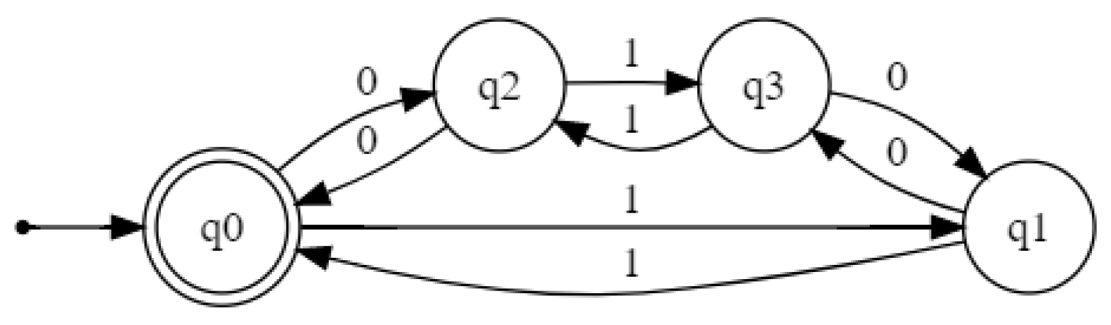
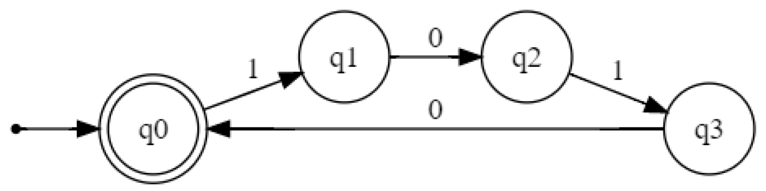
To illustrate this use case, an RNN was trained with data from Tomita’s 5th grammar [36] (Figure 1) until it reached a 100% accuracy both in all data. Similarly, a second network , with the same characteristics, was trained until complete overfitting with sequences from a sublanguage (Figure 2).
The architecture of the networks is depicted in Figure 3 (Network sketches have been generated using Keras utilities https://keras.io/api/utils/model_plotting_utils/, accessed on 5 February 2021). For each layer, its type, name (for clarity), and input/output shapes are shown. In all cases, the first component of the shape vector is the batch size and the last component is the number of features. For three-dimensional shapes, the middle element is the length of the sequence. “?” means that the parameter is not statically fixed but dynamically instantiated at the training phase. The initial layer is a two-dimensional dense embedding of the input. This layer is followed by a sequence-to-sequence subnetwork composed of a 64-dimensional LSTM chained to a 30-dimensional dense layer with a ReLU activation function. The network ends with a classification subnetwork composed of a 62-dimensional LSTM connected to a two-dimensional dense layer with a softmax activation function. This architecture has a total of 42,296 coefficients.
Each network has been trained in a single phase with specific parameters summarized in Table 5. This is the reason why batch size and sequence length have not been fixed in Figure 3 and therefore appear as “?”. The training process of both networks used sets of randomly generated sequences labeled as belonging or not to the corresponding target language. These sets have been split in two parts: 80% for the development set and 20% for the test set. The development set has been further partitioned into 67% for train and 33% for validation.
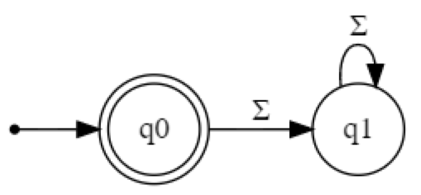
When checking both networks for inclusion in Tomita’s 5th grammar both of them were found to verify the inclusion, passing PAC tests with and . However, when the verification goal was to check , the output was different. In such scenario, on-the-fly verification returned a nonempty DFA, showing that the networks are indeed not equivalent. Figure 4 depicts the DFA approximating the language of their disagreement, that is, the symmetric difference . After further inspection, we found out that does not recognize the empty word .
5.3. An RNN Model of a Cruise Control Software
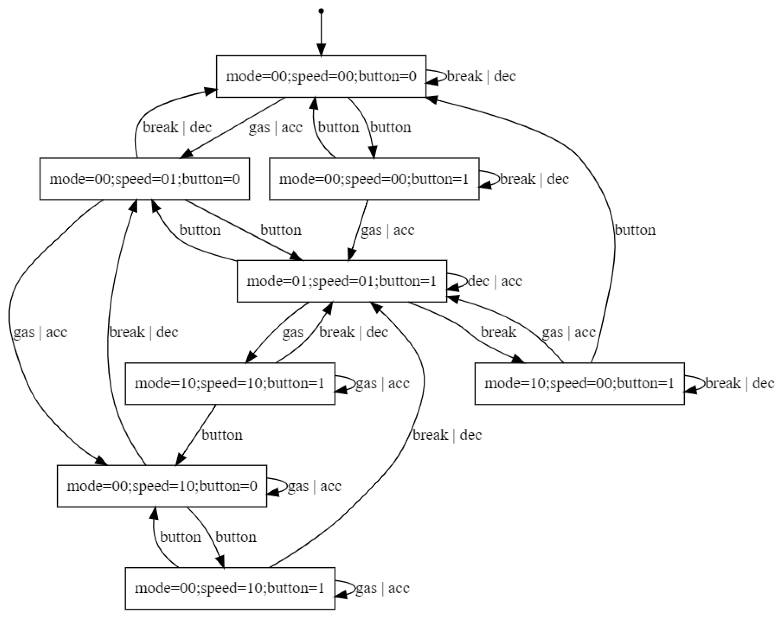
Here, we analyze an RNN trained with sequences from the model of a cruise controller software [37] depicted in Figure 5. In the figure, only the actions and states modeling the normal operation of the controller are shown. All illegal actions are assumed to go to a nonaccepting sink state. The training dataset contained 200,000 randomly generated sequences and labeled as normal and abnormal according to whether they correspond or not to executions of the controller (i.e., they are recognized or not by the DFA in Figure 5). All executions have a length of at most 16 actions. The accuracy of the RNN on a test dataset with 16,000 randomly generated sequences was 99.91%.
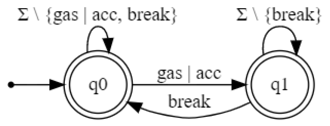
The requirement P to be checked on the RNN is the following: a break action can occur only if action gas|acc has already happened and no other break action has occurred in between. P is modeled by the DFA illustrated in Figure 6.
In this experiment, we compare both approaches, namely our on-the-fly technique vs. post-learning verification.
Every run of on-the-fly verification through learning terminates with perfect tests conjecturing that is empty. Table 6 shows the metrics obtained in these experiments (running times, sample sizes, and ) for different values of the parameters and .
Table 7 shows the metrics for extracting DFA from the RNN. The timeout was set at 200 s. For the first configuration, four out of five runs terminated before the timeout producing automata that exceeded the maximum number of states. Moreover, three of those were shown to violate the requirement. For the second one, there were three out of five successful extractions with all automata exceeding the maximum number of states, while for two the property did not hold. For the third configuration, all runs hit the timeout. Actually, the RNN under analysis classified all the counterexamples returned by the model-checker as negative, that is, they do not belong to its language. In other words, there were false positives. In order to look for true violating sequences, we generated 2 million sequences with for each of the automata H for which the property did not hold. Indeed, none of those sequences was accepted simultaneously by both the RNN under analysis and . Therefore, it is not possible to disprove that the RNN is correct with respect to P as conjectured bye on-the-fly black-box checking. It goes without saying that post-learning verification required considerable more computational effort as a consequence of its misleading verdicts.
The cruise controller case study illustrates an important benefit of our approach vs. post-learning verification: every counterexample produced by on-the-fly property checking is a true witness of being nonempty, while this is certainly false for the latter.
5.4. An RNN Model of an E-Commerce Web Site
In this case study, the target concept is an RNN trained with the purpose of modeling the behavior of a web application for e-commerce. We used a training dataset of 100,000 randomly generated sequences of length smaller than or equal to 16, using a variant of the model in [22,38] to tag the sequences as positive or negative. Purposely, we have modified the model so as to add canary sequences not satisfying the properties to be checked. The RNN achieved 100% accuracy on a test dataset of 16,000 randomly generated sequences. We overfitted to ensure faulty sequences were classified as positive by the RNN. The goal of this experiment was to verify whether on-the-fly black-box checking could successfully unveil whether the RNN learned these misbehaviors.
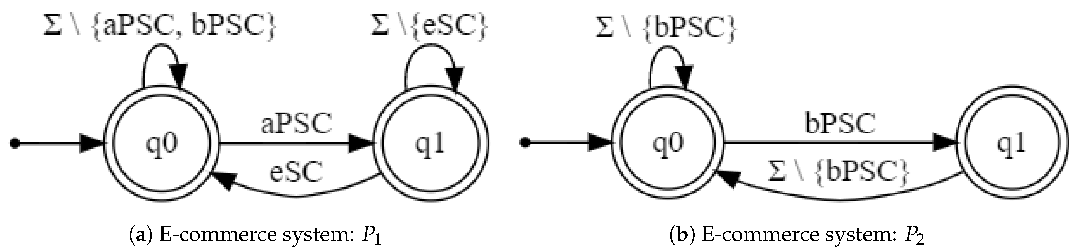
We analyzed the regular properties shown in Figure 7, where labels , , and model the actions (associated with their corresponding buttons) of adding products to the shopping cart, removing all products from the shopping cart, and buying products in the shopping cart, respectively. Requirement , depicted in Figure 7a, states that the e-commerce site must not allow a user to buy products in the shopping cart if the shopping cart does not contain any product. Property , depicted in Figure 7b, requires the system to prevent the user to perform consecutive clicks on the buy products button.
Table 8 shows the metrics obtained for extracting automata. All runs terminated with an with no divergences. Therefore, the extracted automata were -approximations of the RNN. Although we did not perform post-learning verification, these metrics are helpful to compare the computational performance of both approaches.
For each property , , the concept inside the black-box is is . As shown in Table 9, the on-the-fly method correctly asserted that none of the properties were satisfied. It is worth noticing that all experiments terminated with perfect , i.e., . Therefore, the extracted DFA were -approximations of . The average running time to output an automaton of the language of faulty behaviors is bigger than the running time for extracting an automaton of the RNN alone. Nevertheless, the first witness of (i.e., the first witness of nonemptiness) was always found by on-the-fly checking in comparable time.
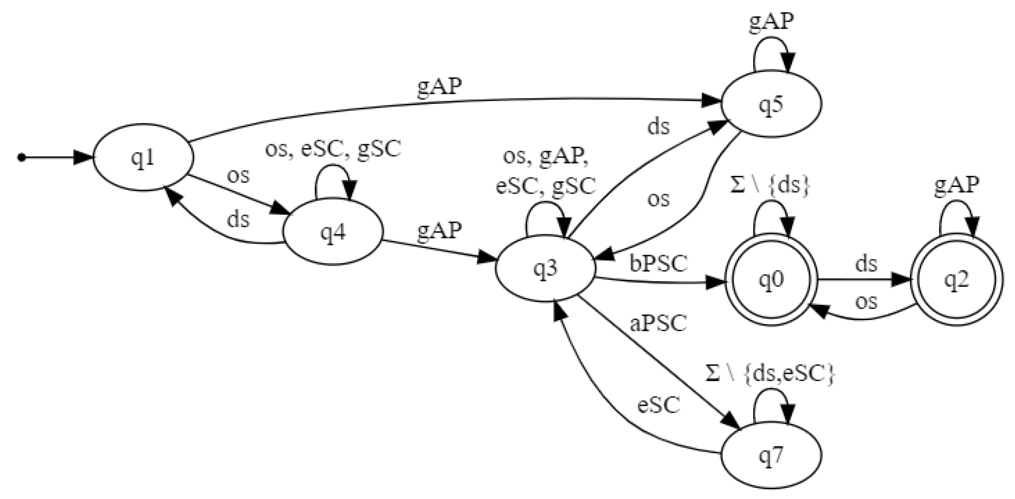
Figure 8 shows an automaton of built by the on-the-fly algorithm. For instance, it reveals that the RNN classifies as correct a sequence where the user opens a session (label event ), consults the list of available products (label gAP), and then buys products (), but the shopping cart is empty: . Indeed, it provides valuable information about possible causes of the error which are helpful to understand it and correcting it, since it makes apparent that every time occurred in an open session, the property was violated.
Figure 9 depicts an automaton for . A sequence showing that is not satified is: . Notice that this automaton shows that is violated as well, since state is reachable without any occurrence of .
5.5. An RNN for Classifying Hadoop File System Logs
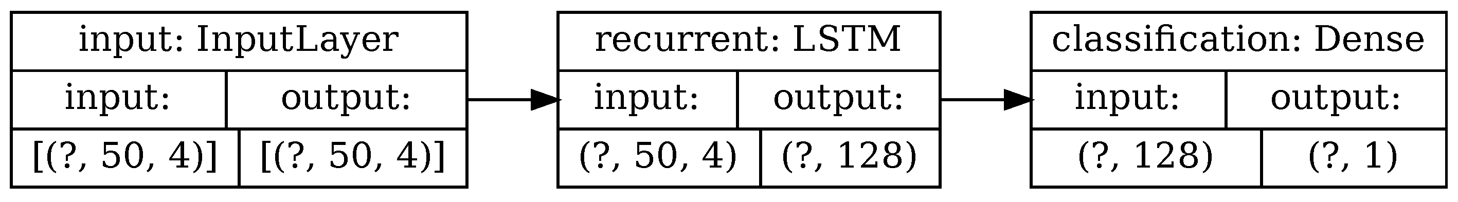
This experiment concerns the analysis of an RNN trained to find anomalies in logs of an application software based on Hadoop Distributed File System (HDFS). Data used in this case study come from [39]. Logs are sequences of natural numbers ranging from 0 to 28 which correspond to different kinds of logged messages. That is, the set of symbols is . The training dataset consists of 4856 normal logs of different lengths. We built an autoregressive network that predicts the probability distribution of symbols at each position in the sequence. Symbols are one-hot encoded. The LSTM layer outputs a 128-dimensional vector which is passed to a 29-dimensional dense layer that outputs the probability distribution of the next symbol. That is, for every position , where T is the length of the sequence, the network outputs a vector , whose i-th position holds the predicted probability of number i to be the t-th symbol in the sequence [40]. Figure 10 shows a sketch of the architecture. This network has 84,637 parameters. The activation function of the last layer is a softmax and the loss function is the corresponding categorical cross-entropy. For the sake of readability, we fixed the sequence length in Figure 10. However, in the actual architecture this parameter is not statically defined.
For each log in the training set we obtained all complete subsequences of length by sliding a window of size 10 from start to end. Overall, there were a total of 56,283 of such subsequences which were split in 80% (36,020 samples) for training and 20% (9006 samples) for validation. A single training phase of five epochs was performed using a learning rate of and a batch size of 30.
In order to build a classifier, the RNN is used to predict the probability of a log. Then, a log is considered to be normal if its predicted probability is beyond a threshold of . Otherwise, it is tagged as anomalous. The performance of the classifier was tested on a perfectly balanced subset of 33,600 samples taken from the test dataset of [39]. No false positives were produced by the classifier which incurred in an overall error of 2.65%.
During an exploratory analysis of the training dataset, we made the following observations. First, there were a subset of numbers, concretely {6, 7, 9, 11–14, 18, 19, 23, 26–28}, that were not present in the normal logs used for training. Let us call this set A for anomalous message types. Second, many logs have a subsequence containing numbers 4 and 21, such that their accumulated count was at most 5, that is, . We analyzed the classifier with the purpose of investigating whether the RNN actually learned these patterns as characteristic of normal logs.
Based on those observations, we defined the following properties. The first statement, , claims that the classifier always labels as anomalous any log containing a number in A. The second one, , says that every log satisfying is classified as normal. As in the case study of the e-commerce, for each property , , the concept inside the black-box is is , where C is the classifier. It is worth mentioning that C is indeed the composition of an RNN with the decision function that labels logs according to the probability output by the RNN.
Table 10 shows the results obtained with on-the-fly checking through learning. As in previous experiments, five runs of the algorithm were executed for each configuration. All runs terminated with perfect tests. Hence, all output hypotheses were -approximations of .
On one hand, property is satisfied by C with PAC guarantees. On the contrary, all runs of the algorithm for returned a nonempty automaton and a set of the logs that violate . Therefore, we conclude that C actually classifies as normal some logs containing numbers in A. Figure 11 depicts the automaton obtained for . It helps to understand the errors of C. For example, it reveals that C labels as normal a log that contains an occurrence of a number in A in its prefix of length 2. This behavior is captured by paths , , and . Indeed, this outcome highlights the importance of verification, since it revealed a clear mismatch with the results observed on the test dataset where C all logs containing numbers in A were labelled as anomalous because C reported no false positives whatsoever.
5.6. An RNN for Recognizing TATA-Boxes in DNA Promoter Sequences
DNA promoter sequences are in charge of controlling gene activation or repression. A TATA-box is a promoter subsequence with the special role of indicating other molecules the starting place of the transcription. A TATA-box is a subsequence having a length of six base pairs (bp). It is located upstream close to the gene transcription start site (TSS) from positions −30 bp to −25 bp (TSS is located at +1 bp). It is characterized by the fact that the accumulated number of occurrences of A’s and T’s is larger than that of C’s and G’s.
Recently, RNN-based techniques for recognizing TATA-box promoter regions in DNA sequences have been proposed [16]. Therefore, it is of interest to check whether an RNN classifies as positive sequences having a TATA-box and as negative those not having it. In terms of a formal language, the property can be characterized as the set of sequences with a subsequence v of length 6 from −30 bp to −25 bp such that , where is the number of occurrences of in v.
For that purpose, we trained an RNN until achieving 100% accuracy on the training data consisting of 16,455 aligned TATA and non-TATA promoter sequences of human DNA extracted from the online database EPDnew (https://epd.epfl.ch/index.php, accessed 5 February 2021). All sequences have a total length of 50 and end at the TSS. Overall, there were 2067 sequences with TATA boxes and 14,388 sequences without. The LSTM layer had a 128-dimensional output. In this case, training was performed on a single phase with a learning rate of and a batch size of 64. No validation nor test sets were used. Figure 12 shows a graphical sketch of the model. The input dimension is given by the batch size, the length of the sequence, and the number of symbols.
Table 11 shows the results obtained only with the on-the-fly approach. Indeed, every attempt to learn a DFA of the RNN C caused Bounded- to terminate with a timeout. Therefore, this case study illustrates the case where post-learning verification is not feasible while on-the-fly checking is. It turns out that all executions concluded that the empty language was an -approximation of the black-box . Thus, C verifies the requirement with PAC guarantees. It is worth noticing that in the last reported experiment, with and equal to , the sample used for checking equivalence was about an order of magnitude bigger than the dataset used for training.
6. Related Work
Regular inference on RNN can be considered to be a kind of rule extraction technique [41], where the rules that are extracted are represented by a DFA. Several different approaches for extracting automata out of RNN have been proposed. The method developed in [19,20] resorts to quantizing the hidden values of the network states and to using clustering for grouping them into automata states. The algorithm discussed in [18] combines and partition refinement. The equivalence query compares the proposed hypothesis with an abstract representation of the network obtained by refining a partition of its internal states. Those techniques are white box as they rely on some level of knowledge of the internal structure of the network. They can be applied for post-learning verification but they are not directly usable for on-the-fly black-box property checking. None of them provide provable PAC-guarantees on the generated automata.
There are a number of works that perform white-box, compositional, automata-theoretic verification of temporal properties by learning assumptions but require an external decision procedure [42,43,44]. Verification of regular properties of systems modeled as nonregular languages (expressed as automata equipped with FIFO queues) by means of learning DFA is proposed in [45]. However, the algorithm is white-box, it relies on a state-based representation of the FIFO automaton, and it requires being able to compute successor states of words by transitions of the target automata, which is by no means feasible for RNN. Our approach also differs from [46], since this work proposes an iterative technique for regular model-checking based on Trakhtenbrot-Barzdin passive learning algorithm [47] which requires generating complete datasets of positive and negative sequences.
Regarding BBC-based approaches, on-the-fly property checking through learning differs from on-the-fly BBC [26] which consists on a strategy for seeking paths in the automaton of the requirement. In this context, it is worth mentioning test case generation with learning based testing (LBT) [48]. LBT works by incrementally constructing hypotheses of the system under test (SUT) and model-checking them against a requirement. The counterexamples returned by the external model-checker become the test cases. LBT does not rely on PAC-learning and does not provide provable probabilistic guarantees on the hypothesis. Somehow, this issue has been partially studied in [49] but at the price of relaxing the black-box setting by observing and storing the SUT internal state.
White-box verification and testing of safety properties on feed-forward (FFNN) and convolutional (CNN) neural networks based on Linear Programming (LP) and Satisfiability Modulo Theories (SMT) has been explored in several works, for instance [50,51,52,53]. Reluplex [51] is a problem-specific SMT solver which handles ReLU constraints. The method in [52] exhaustively searches for adversarial misclassifications, propagating the analysis from one layer to the other directly through the source code. Several works have approached the problem of checking robustness, which is a specific property that evaluates ANN resilience to adversarial examples. DeepSafe [54] is a white-box tool for checking robustness based on clustering and constraint solvers. A black-box approach for robustness testing is developed in [55]. Those approaches have been applied for image classification with deep convolutional and dense layers but not for RNN over symbolic sequences.
In the case of RNN, a white-box, post-learning approach for adversarial accuracy verification is presented in [56]. The technique relies on extracting DFA from RNN but does not provide PAC guarantees. Besides, no real-life applications have been analyzed but only RNN trained with sequences of 0 s and 1 s from academic DFA [36]. In [57] white-box RNN verification is done by generating a series of abstractions. Specifically, the method strongly relies on the internal structure and weights of the RNN to generate a FFNN, which is proven to compute the same output. Then, reachability analysis is performed resorting to LP and SMT. RNSVerify [58] implements white-box verification of safety properties by unrolling the RNN and resorting to LP to solve a system of constraints. The method strongly relies on the internal structure and weight matrices of the RNN. Overall, these techniques are white-box and are not able to handle arbitrary properties over sequences. Moreover, they do not address the problem of producing interpretable characterizations of the errors incurred by the RNN under analysis.
A related but different approach is statistical model checking (SMC) [59,60]. SMC seeks to check whether a stochastic system satisfies a (possibly stochastic) property with a probability beyond some threshold. However, in our context, both the RNN is deterministic and the property are deterministic. That is, any sequence either satisfies or not. Moreover, our technique works by PAC-learning an arbitrary language expressed as a formula , where C is an RNN.
7. Conclusions
This paper explores the problem of checking properties of RNN devoted to sequence classification over symbolic alphabets in a black-box setting. The approach is not restricted to any particular class of RNN or property. Besides it is on-the-fly because it does not construct a model of the RNN on which the property is verified. The key idea is to express the verification problem on an RNN C as a formula such that its language is empty if and only if C does not satisfy the requirement and apply a PAC-learning algorithm for learning . On one hand, if the resulting DFA is empty, the algorithm provides PAC-guarantees about the language being itself empty. On the other, if the output DFA is not empty, it provides an actual sequence of C that belongs to . Besides, the DFA itself serves as an approximate characterization of the set of all sequences in . For instance, our method can be used to verify whether an RNN C satisfies a linear-time temporal property P by checking . Since the approach does not require computing the complement, it can also be applied to verify nonregular properties expressed, for instance, as context-free grammars, and to check equivalence between RNN, as illustrated in Section 5.
On-the-fly checking through learning has several advantages with respect to performs post-learning verification. When the learnt language that approximates is nonempty, the algorithm provides true evidence of the failure by means of concrete counterexamples. In addition, the algorithm outputs an interpretable characterization of an approximation of the set of incorrect behaviors. Besides, it allows checking properties, with PAC guarantees, for which no decision procedure exists. Moreover, the experimental results on a number of case studies from different application domains provide empirical evidence that the on-the-fly approach typically outperforms post-learning verification if the requirement is probably approximately satisfied.
Last but not least, Theorem 1 provides an upper bound of the error incurred by any DFA returned by Bounded-. Hence, this paper also improves the previously known theoretical results regarding the probabilistic guarantees of this learning algorithm [22].
Author Contributions
F.M. and S.Y. equally contributed to the theoretical, experimental results and writing. R.V. contributed to prototyping and experimentation. All authors have read and agreed to the published version of the manuscript.
Funding
This research was partially funded by ICT4V—Information and Communication Technologies for Verticals grant number POS_ICT4V_2016_1_15, and ANII—Agencia Nacional de Investigación e Innovación grant numbers FSDA_1_2018_1_154419 and FMV_1_2019_1_155913.
Data Availability Statement
Data sources used in this work were referenced throughout the article.
Conflicts of Interest
The authors declare no conflict of interest.
References
- Miller, T. Explanation in artificial intelligence: Insights from the social sciences. Artif. Intell. 2019, 267, 1–38. [Google Scholar] [CrossRef]
- Biran, O.; Cotton, C.V. Explanation and Justification in Machine Learning: A Survey. In Proceedings of the IJCAI Workshop on Explainable Artificial Intelligence (XAI), Melbourne, Australia 19–25 August 2017. [Google Scholar]
- Ahmad, M.; Teredesai, A.; Eckert, C. Interpretable Machine Learning in Healthcare. In Proceedings of the 2018 IEEE International Conference on Healthcare Informatics (ICHI); IEEE Computer Society: Los Alamitos, CA, USA, 2018; p. 447. [Google Scholar] [CrossRef]
- LeCun, Y.; Bengio, Y.; Hinton, G. Deep learning. Nature 2015, 521, 436–444. [Google Scholar] [CrossRef]
- Ribeiro, M.T.; Singh, S.; Guestrin, C. “Why Should I Trust You?”: Explaining the Predictions of Any Classifier. In Proceedings of the SIGKDD Knowledge Discovery and Data Mining, San Francisco, CA, USA, 13–17 August 2016; pp. 1135–1144. [Google Scholar]
- Scheiner, N.; Appenrodt, N.; Dickmann, J.; Sick, B. Radar-based Road User Classification and Novelty Detection with Recurrent Neural Network Ensembles. In Proceedings of the 2019 IEEE Intelligent Vehicles Symposium (IV), Paris, France, 9–12 June 2019; pp. 722–729. [Google Scholar]
- Kocić, J.; Jovičić, N.; Drndarević, V. An End-to-End Deep Neural Network for Autonomous Driving Designed for Embedded Automotive Platforms. Sensors 2019, 19, 2064. [Google Scholar] [CrossRef] [PubMed] [Green Version]
- Kim, J.; Kim, J.; Thu, H.L.T.; Kim, H. Long short term memory recurrent neural network classifier for intrusion detection. In Proceedings of the 2016 International Conference on Platform Technology and Service (PlatCon), Jeju, Korea, 15–17 February 2016; pp. 1–5. [Google Scholar]
- Yin, C.; Zhu, Y.; Fei, J.; He, X. A deep learning approach for intrusion detection using recurrent neural networks. IEEE Access 2017, 5, 21954–21961. [Google Scholar] [CrossRef]
- Pascanu, R.; Stokes, J.W.; Sanossian, H.; Marinescu, M.; Thomas, A. Malware classification with recurrent networks. In Proceedings of the 2015 IEEE International Conference on Acoustics, Speech and Signal Processing (ICASSP), South Brisbane, QLD, Australia, 19–24 April 2015; pp. 1916–1920. [Google Scholar]
- Rhode, M.; Burnap, P.; Jones, K. Early Stage Malware Prediction Using Recurrent Neural Networks. Comput. Secur. 2017, 77, 578–594. [Google Scholar] [CrossRef]
- Vinayakumar, R.; Alazab, M.; Soman, K.; Poornachandran, P.; Venkatraman, S. Robust Intelligent Malware Detection Using Deep Learning. IEEE Access 2019, 7, 46717–46738. [Google Scholar] [CrossRef]
- Singh, D.; Merdivan, E.; Psychoula, I.; Kropf, J.; Hanke, S.; Geist, M.; Holzinger, A. Human activity recognition using recurrent neural networks. In International Cross-Domain Conference for Machine Learning and Knowledge Extraction; Springer: Berlin/Heidelberg, Germany, 2017; pp. 267–274. [Google Scholar]
- Choi, E.; Bahadori, M.T.; Schuetz, A.; Stewart, W.F.; Sun, J. Doctor AI: Predicting Clinical Events via Recurrent Neural Networks. In Proceedings of the 1st Machine Learning for Healthcare Conference; Doshi-Velez, F., Fackler, J., Kale, D., Wallace, B., Wiens, J., Eds.; PMLR: Boston, MA, USA, 2016; Volume 56, pp. 301–318. [Google Scholar]
- Pham, T.; Tran, T.; Phung, D.; Venkatesh, S. Predicting healthcare trajectories from medical records: A deep learning approach. J. Biomed. Inform. 2017, 69, 218–229. [Google Scholar] [CrossRef]
- Oubounyt, M.; Louadi, Z.; Tayara, H.; Chong, K.T. DeePromoter: Robust promoter predictor using deep learning. Front. Genet. 2019, 10, 286. [Google Scholar] [CrossRef] [PubMed] [Green Version]
- Clarke, E.M.; Grumberg, O.; Peled, D.A. Model Checking; MIT Press: Cambridge, MA, USA, 1999. [Google Scholar]
- Weiss, G.; Goldberg, Y.; Yahav, E. Extracting Automata from Recurrent Neural Networks Using Queries and Counterexamples. In Proceedings of the International Conference on Machine Learning ICML, PMLR, Stockholm, Sweden, 10–15 July 2018; Volume 80. [Google Scholar]
- Wang, Q.; Zhang, K.; Ororbia, A.G., II; Xing, X.; Liu, X.; Giles, C.L. An Empirical Evaluation of Rule Extraction from Recurrent Neural Networks. Neural Comput. 2018, 30, 2568–2591. [Google Scholar] [CrossRef]
- Wang, Q.; Zhang, K.; Ororbia, A.G., II; Xing, X.; Liu, X.; Giles, C.L. A Comparison of Rule Extraction for Different Recurrent Neural Network Models and Grammatical Complexity. arXiv 2018, arXiv:1801.05420. [Google Scholar]
- Merrill, W. Sequential neural networks as automata. arXiv 2019, arXiv:1906.01615. [Google Scholar]
- Mayr, F.; Yovine, S. Regular Inference on Artificial Neural Networks. In Machine Learning and Knowledge Extraction; Springer: Cham, Switzerland, 2018; pp. 350–369. [Google Scholar]
- Valiant, L.G. A Theory of the Learnable. Commun. ACM 1984, 27, 1134–1142. [Google Scholar] [CrossRef] [Green Version]
- Odena, A.; Olsson, C.; Andersen, D.; Goodfellow, I.J. TensorFuzz: Debugging Neural Networks with Coverage-Guided Fuzzing. In Proceedings of the International Conference on Machine Learning ICML, PMLR, Long Beach, CA, USA, 9–15 June 2019; Volume 97, pp. 4901–4911. [Google Scholar]
- Mayr, F.; Visca, R.; Yovine, S. On-the-fly Black-Box Probably Approximately Correct Checking of Recurrent Neural Networks. In Proceedings of the 4th IFIP TC 5, TC 12, WG 8.4, WG 8.9, WG 12.9 International Cross-Domain Conference on Machine Learning and Knowledge Extraction (CD-MAKE 2020), Dublin, Ireland, 25–28 August 2020; Holzinger, A., Kieseberg, P., Tjoa, A.M., Weippl, E.R., Eds.; Lecture Notes in Computer Science. Springer: Berlin/Heidelberg, Germany, 2020; Volume 12279, pp. 343–363. [Google Scholar] [CrossRef]
- Peled, D.; Vardi, M.Y.; Yannakakis, M. Black box checking. J. Autom. Lang. Comb. 2002, 7, 225–246. [Google Scholar]
- Angluin, D. Computational Learning Theory: Survey and Selected Bibliography. In Proceedings of the Twenty-Fourth Annual ACM Symposium on Theory of Computing, Victoria, BC, Canada, 4–6 May 1992; pp. 351–369. [Google Scholar]
- Ben-David, S.; Shalev-Shwartz, S. Understanding Machine Learning: From Theory to Algorithms; Cambridge University Press: Cambridge, UK, 2014. [Google Scholar]
- Angluin, D. Learning Regular Sets from Queries and Counterexamples. Inf. Comput. 1987, 75, 87–106. [Google Scholar] [CrossRef] [Green Version]
- Siegelmann, H.T.; Sontag, E.D. On the Computational Power of Neural Nets. In Proceedings of the twenty-fourth annual ACM symposium on Theory of Computing, Victoria, BC, Canada, 4–6 May 1992; pp. 440–449. [Google Scholar]
- Suzgun, M.; Belinkov, Y.; Shieber, S.M. On Evaluating the Generalization of LSTM Models in Formal Languages. arXiv 2018, arXiv:1811.01001. [Google Scholar]
- Heinz, J.; de la Higuera, C.; van Zaanen, M. Formal and Empirical Grammatical Inference. In Proceedings of the ACL Annual Meeting, ACL, Minneapolis, MN, USA, 10–13 November 2011; pp. 2:1–2:83. [Google Scholar]
- Hochreiter, S.; Schmidhuber, J. Long Short-Term Memory. Neural Comput. 1997, 9, 1735–1780. [Google Scholar] [CrossRef]
- Hao, Y.; Merrill, W.; Angluin, D.; Frank, R.; Amsel, N.; Benz, A.; Mendelsohn, S. Context-free transductions with neural stacks. arXiv 2018, arXiv:1809.02836. [Google Scholar]
- Hopcroft, J.E.; Motwani, R.; Ullman, J.D. Introduction to automata theory, languages, and computation. ACM Sigact News 2001, 32, 60–65. [Google Scholar] [CrossRef]
- Tomita, M. Dynamic Construction of Finite Automata from examples using Hill-climbing. In Proceedings of the Fourth Annual Conference of the Cognitive Science Society, Vancouver, BC, Canada, 26–29 July 2006; pp. 105–108. [Google Scholar]
- Meinke, K.; Sindhu, M.A. LBTest: A Learning-Based Testing Tool for Reactive Systems. In Proceedings of the 2013 IEEE Sixth International Conference on Software Testing, Verification and Validation, Luxembourg, 18–22 March 2013; pp. 447–454. [Google Scholar]
- Merten, M. Active Automata Learning for Real Life Applications. Ph.D. Thesis, Technischen Universität Dortmund, Dortmund, Germany, 2013. [Google Scholar]
- Du, M.; Li, F.; Zheng, G.; Srikumar, V. DeepLog: Anomaly Detection and Diagnosis from System Logs through Deep Learning. In Proceedings of the 2017 ACM SIGSAC Conference on Computer and Communications Security, CCS 2017, Dallas, TX, USA, 30 October–3 November 2017; pp. 1285–1298. [Google Scholar]
- Bengio, Y.; Ducharme, R.; Vincent, P.; Janvin, C. A Neural Probabilistic Language Model. J. Mach. Learn. Res. 2003, 3, 1137–1155. [Google Scholar]
- Craven, M.W. Extracting Comprehensible Models from Trained Neural Networks. Ph.D. Thesis, The University of Wisconsin, Madison, WI, USA, 1996. AAI9700774. [Google Scholar]
- Cobleigh, J.M.; Giannakopoulou, D.; Păsăreanu, C.S. Learning assumptions for compositional verification. In Proceedings of the International Conference on Tools and Algorithms for the Construction and Analysis of Systems; Springer: Berlin/Heidelberg, Germany, 2003; pp. 331–346. [Google Scholar]
- Alur, R.; Madhusudan, P.; Nam, W. Symbolic compositional verification by learning assumptions. In Proceedings of the International Conference on Computer Aided Verification; Springer: Berlin/Heidelberg, Germany, 2005; pp. 548–562. [Google Scholar]
- Feng, L.; Han, T.; Kwiatkowska, M.; Parker, D. Learning-based compositional verification for synchronous probabilistic systems. In Proceedings of the International Symposium on Automated Technology for Verification and Analysis; Springer: Berlin/Heidelberg, Germany, 2011; pp. 511–521. [Google Scholar]
- Vardhan, A.; Sen, K.; Viswanathan, M.; Agha, G. Actively learning to verify safety for FIFO automata. In Foundations of Software Technology and Theoretical Computer Science; Springer: Berlin/Heidelberg, Germany, 2004; pp. 494–505. [Google Scholar]
- Habermehl, P.; Vojnar, T. Regular Model Checking Using Inference of Regular Languages. ENTCS 2004, 138, 21–36. [Google Scholar] [CrossRef]
- Trakhtenbrot, B.A.; Barzdin, I.M. Finite Automata: Behavior and Synthesis; North-Holland: Amsterdam, The Netherlands, 1973; 321p. [Google Scholar]
- Meinke, K. Learning-based testing: Recent progress and future prospects. In Machine Learning for Dynamic Software Analysis: Potentials and Limits; Springer: Berlin/Heidelberg, Germany, 2018; pp. 53–73. [Google Scholar]
- Meijer, J.; van de Pol, J. Sound black-box checking in the LearnLib. Innov. Syst. Softw. Eng. 2019, 15, 267–287. [Google Scholar] [CrossRef] [Green Version]
- Pulina, L.; Tacchella, A. Challenging SMT solvers to verify neural networks. AI Commun. 2012, 25, 117–135. [Google Scholar] [CrossRef]
- Katz, G.; Barrett, C.W.; Dill, D.L.; Julian, K.; Kochenderfer, M.J. Reluplex: An Efficient SMT Solver for Verifying Deep Neural Networks. In Proceedings of the International Conference on Computer Aided Verification; Springer: Berlin/Heidelberg, Germany, 2017; Volume 10426, pp. 97–117. [Google Scholar]
- Huang, X.; Kwiatkowska, M.; Wang, S.; Wu, M. Safety Verification of Deep Neural Networks. In Proceedings of the International Conference on Computer Aided Verification; Springer: Berlin/Heidelberg, Germany, 2017; Volume 10426, pp. 3–29. [Google Scholar]
- Ehlers, R. Formal Verification of Piece-Wise Linear Feed-Forward Neural Networks. In Proceedings of the International Symposium on Automated Technology for Verification and Analysis; Springer: Cham, Switzerland, 2017; Volume 10482, pp. 269–286. [Google Scholar]
- Gopinath, D.; Katz, G.; Pasareanu, C.S.; Barrett, C.W. DeepSafe: A Data-Driven Approach for Assessing Robustness of Neural Networks. In Proceedings of the 16th International Symposium on Automated Technology for Verification and Analysis (ATVA 2018); Los Angeles, CA, USA, 7–10 October 2018, Lahiri, S.K., Wang, C., Eds.; Lecture Notes in Computer Science; Springer: Berlin/Heidelberg, Germany, 2018; Volume 11138, pp. 3–19. [Google Scholar] [CrossRef]
- Wicker, M.; Huang, X.; Kwiatkowska, M. Feature-guided black-box safety testing of deep neural networks. In Proceedings of the International Conference on Tools and Algorithms for the Construction and Analysis of Systems; Springer: Berlin/Heidelberg, Germany, 2018; pp. 408–426. [Google Scholar]
- Wang, Q.; Zhang, K.; Liu, X.; Giles, C.L. Verification of Recurrent Neural Networks Through Rule Extraction. In Proceedings of the AAAI Spring Symposium on Verification of Neural Networks (VNN19), Stanford, CA, USA, 25–27 March 2019. [Google Scholar]
- Kevorchian, A. Verification of Recurrent Neural Networks. Master’s Thesis, Imperial College London, London, UK, 2018. [Google Scholar]
- Akintunde, M.E.; Kevorchian, A.; Lomuscio, A.; Pirovano, E. Verification of RNN-Based Neural Agent-Environment Systems. In Proceedings of the AAAI Conference on Artificial Intelligence, AAAI, New York, NY, USA, 7–12 February 2019; pp. 6006–6013. [Google Scholar]
- Legay, A.; Lukina, A.; Traonouez, L.M.; Yang, J.; Smolka, S.A.; Grosu, R. Statistical Model Checking. In Computing and Software Science: State of the Art and Perspectives; Springer: Cham, Switzerland, 2019; pp. 478–504. [Google Scholar]
- Agha, G.; Palmskog, K. A Survey of Statistical Model Checking. ACM Trans. Model. Comput. Simul. 2018, 28, 1–39. [Google Scholar] [CrossRef]
Figure 1.
DFA recognizing Tomita’s 5th grammar.

Figure 2.
DFA recognizing a sublanguage of Tomita’s 5th grammar.

Figure 3.
Sketch of the architecture used for Tomita’s 5th grammar and its variant.

Figure 4.
DFA approximating .

Figure 5.
Cruise controller: DFA model.

Figure 6.
Cruise controller: Property P.

Figure 7.
E-commerce system: Automata of the analyzed requirements.

Figure 8.
E-commerce system: Automaton for .

Figure 9.
E-commerce system: Automaton for .
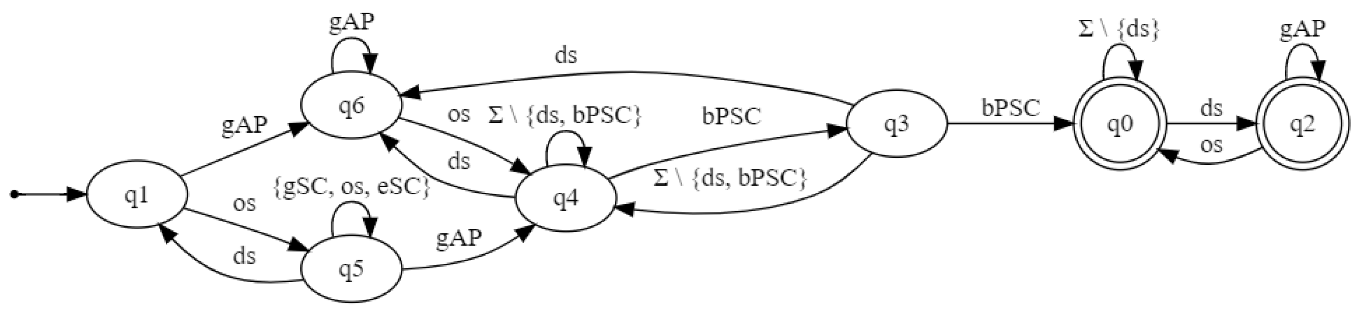
Figure 10.
Sketch of the architecture of the language model of Hadoop Distributed File System (HDFS) logs.
Figure 10.
Sketch of the architecture of the language model of Hadoop Distributed File System (HDFS) logs.

Figure 11.
Hadoop file system logs: Automaton for obtained with and .
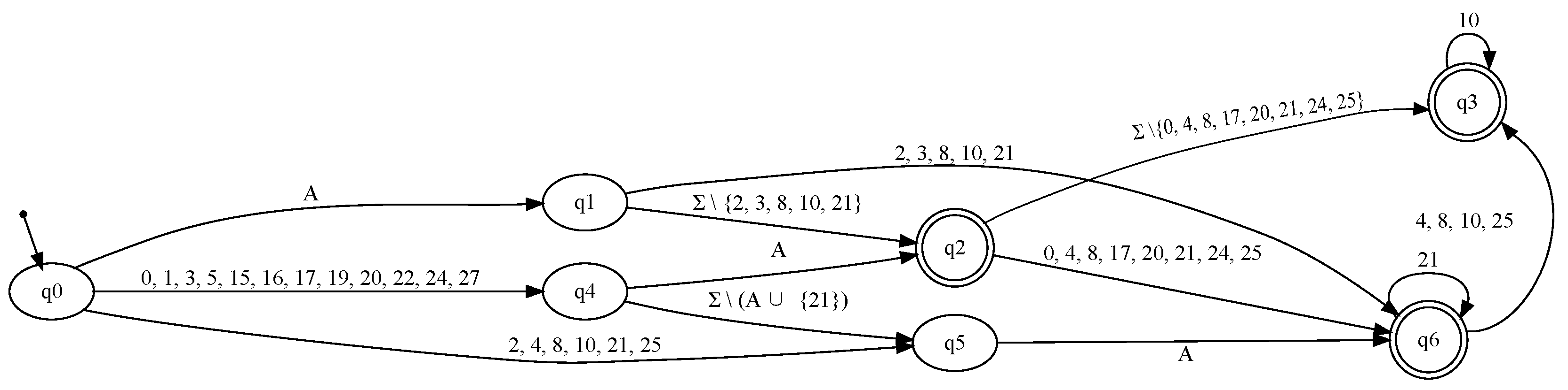
Figure 12.
Sketch of the architecture of the TATA-Box classification network


Table 1.
Dyck 1: Probably approximately correct (PAC) deterministic finite automata (DFA) extraction from recurrent neural networks (RNN).
Table 1.
Dyck 1: Probably approximately correct (PAC) deterministic finite automata (DFA) extraction from recurrent neural networks (RNN).
| Parameters | Running Time (in s) | Mean Sample Size | |||
|---|---|---|---|---|---|
| min | max | mean | |||
| 0.005 | 0.005 | 1.984 | 7.205 | 3.072 | 1899 |
| 0.0005 | 0.005 | 3.713 | 10.445 | 5.997 | 20,093 |
| 0.00005 | 0.005 | 7.982 | 30.470 | 9.997 | 203,007 |
| 0.00005 | 0.0005 | 8.128 | 36.621 | 9.919 | 249,059 |
| 0.00005 | 0.00005 | 9.625 | 41.884 | 12.185 | 295,111 |
Table 2.
Dyck 1: On-the-fly verification of RNN.
| Parameters | Running Time (in s) | First Positive | Mean Sample Size | ||||
|---|---|---|---|---|---|---|---|
| min | max | mean | |||||
| 0.005 | 0.005 | 0.004 | 0.012 | 0.006 | - | 1476 | |
| 0.0005 | 0.005 | 0.051 | 0.125 | 0.067 | - | 14,756 | |
| 0.00005 | 0.005 | 0.682 | 0.833 | 0.747 | - | 147,556 | |
| 0.00005 | 0.0005 | 1.164 | 1.595 | 1.340 | - | 193,607 | |
| 0.00005 | 0.00005 | 1.272 | 1.809 | 1.386 | - | 239,659 | |
| 0.005 | 0.005 | 0.031 | 34.525 | 5.762 | 0.099 | 1948 | |
| 0.0005 | 0.005 | 0.397 | 37.846 | 10.245 | 0.084 | 20,370 | |
| 0.00005 | 0.005 | 4.713 | 30.714 | 6.547 | 0.825 | 206,473 | |
| 0.005 | 0.005 | 0.025 | 0.966 | 0.302 | 0.006 | 1899 | |
| 0.0005 | 0.005 | 0.267 | 1.985 | 0.787 | 0.070 | 20,093 | |
| 0.00005 | 0.005 | 4.376 | 6.479 | 4.775 | 0.764 | 203,007 | |
Table 3.
Dyck 2: PAC DFA extraction from RNN.
| Parameters | Running Time (in s) | Mean Sample Size | Mean | |||
|---|---|---|---|---|---|---|
| Min | Max | Mean | ||||
| 0.005 | 0.005 | 2.753 | 149.214 | 19.958 | 1795 | 0.00559 |
| 0.0005 | 0.005 | 23.343 | 300.000 | 105.367 | 18,222 | 0.04432 |
| 0.00005 | 0.005 | 42.518 | 139.763 | 77.652 | 186,372 | 0.16248 |
Table 4.
Dyck 2: On-the-fly verification of RNN.
| Parameters | Running Time (in s) | First Positive | Mean Sample Size | Mean | |||
|---|---|---|---|---|---|---|---|
| Min | Max | Mean | |||||
| 0.005 | 0.005 | 0.004 | 122.388 | 24.483 | 90.285 | 1504 | 0.00618 |
| 0.0005 | 0.005 | 55.084 | 300.000 | 215.508 | 42.462 | 16,604 | 0.00895 |
| 0.00005 | 0.005 | 0.695 | 324.144 | 158.195 | 4.545 | 166,040 | 0.00005 |
Table 5.
Training parameters used for Tomita’s 5th grammar and its variant.
| Network | Dataset Size | Batch Size | Sequence Length | Learning Rate |
|---|---|---|---|---|
| 5K | 30 | 15 | 0.01 | |
| 1M | 100 | 10 | 0.001 |
Table 6.
Cruise controller: On-the-fly black-box checking.
| Parameters | Running Times (in s) | First Positive | Mean Sample Size | |||
|---|---|---|---|---|---|---|
| Min | Max | Mean | ||||
| 0.01 | 0.01 | 0.003 | 0.006 | 0.004 | - | 669 |
| 0.001 | 0.01 | 0.061 | 0.096 | 0.075 | - | 6685 |
| 0.0001 | 0.01 | 0.341 | 0.626 | 0.497 | - | 66,847 |
Table 7.
Cruise controller: Automaton extraction.
| Parameters | Running Times (in s) | Mean Sample Size | Mean | |||
|---|---|---|---|---|---|---|
| Min | Max | Mean | ||||
| 0.01 | 0.01 | 11.633 | 200.000 | 67.662 | 808 | 0.07329 |
| 0.001 | 0.01 | 52.362 | 200.000 | 135.446 | 8071 | 0.22684 |
| 0.0001 | 0.01 | - | - | - | - | - |
Table 8.
E-commerce: PAC DFA extraction from RNN.
| Parameters | Running Times (in s) | Mean Sample Size | |||
|---|---|---|---|---|---|
| Min | Max | Mean | |||
| 0.01 | 0.01 | 16.863 | 62.125 | 36.071 | 863 |
| 0.001 | 0.01 | 6.764 | 9.307 | 7.864 | 8487 |
| 0.0001 | 0.01 | 18.586 | 41.137 | 30.556 | 83,482 |
Table 9.
E-commerce: On-the-fly verification of RNN.
| Parameters | Running Times (in s) | First Positive | Mean Sample Size | ||||
|---|---|---|---|---|---|---|---|
| Min | Max | Mean | |||||
| 0.01 | 0.01 | 87.196 | 312.080 | 174.612 | 3.878 | 891 | |
| 0.001 | 0.01 | 0.774 | 203.103 | 102.742 | 0.744 | 9181 | |
| 0.0001 | 0.01 | 105.705 | 273.278 | 190.948 | 2.627 | 94,573 | |
| 0.01 | 0.01 | 0.002 | 487.709 | 148.027 | 80.738 | 752 | |
| 0.001 | 0.01 | 62.457 | 600.000 | 428.400 | 36.606 | 8765 | |
| 0.0001 | 0.01 | 71.542 | 451.934 | 250.195 | 41.798 | 87,641 | |
Table 10.
Hadoop file system logs: On-the-fly verification.
| Prop | Parameters | Running Times (in s) | First Positive | Mean Sample Size | |||
|---|---|---|---|---|---|---|---|
| Min | Max | Mean | |||||
| 0.01 | 0.01 | 209.409 | 1,121.360 | 555.454 | 5.623 | 932 | |
| 0.001 | 0.001 | 221.397 | 812.764 | 455.660 | 1.321 | 12,037 | |
| 0.01 | 0.01 | 35.131 | 39.762 | 37.226 | - | 600 | |
| 0.001 | 0.001 | 252.202 | 257.312 | 254.479 | - | 8295 | |
Table 11.
TATA-box: On-the-fly verification of RNN.
| Parameters | Running Times (in s) | Mean Sample Size | |||
|---|---|---|---|---|---|
| Min | Max | Mean | |||
| 0.01 | 0.01 | 5.098 | 5.259 | 5.168 | 600 |
| 0.001 | 0.001 | 65.366 | 66.479 | 65.812 | 8295 |
| 0.0001 | 0.0001 | 865.014 | 870.663 | 867.830 | 105,967 |
Publisher’s Note: MDPI stays neutral with regard to jurisdictional claims in published maps and institutional affiliations. |
© 2021 by the authors. Licensee MDPI, Basel, Switzerland. This article is an open access article distributed under the terms and conditions of the Creative Commons Attribution (CC BY) license (http://creativecommons.org/licenses/by/4.0/).
Share and Cite
MDPI and ACS Style
Mayr, F.; Yovine, S.; Visca, R. Property Checking with Interpretable Error Characterization for Recurrent Neural Networks. Mach. Learn. Knowl. Extr. 2021, 3, 205-227. https://0-doi-org.brum.beds.ac.uk/10.3390/make3010010
AMA Style
Mayr F, Yovine S, Visca R. Property Checking with Interpretable Error Characterization for Recurrent Neural Networks. Machine Learning and Knowledge Extraction. 2021; 3(1):205-227. https://0-doi-org.brum.beds.ac.uk/10.3390/make3010010
Chicago/Turabian StyleMayr, Franz, Sergio Yovine, and Ramiro Visca. 2021. "Property Checking with Interpretable Error Characterization for Recurrent Neural Networks" Machine Learning and Knowledge Extraction 3, no. 1: 205-227. https://0-doi-org.brum.beds.ac.uk/10.3390/make3010010