Article

Dynamic Measurements with the Bicone Interfacial Shear Rheometer: The Effects of the Numerical Implementation of the Interfacial Boundary Condition

by
Pablo Sánchez-Puga
1,*,†,
Javier Tajuelo
2,†,
Juan Manuel Pastor
3,† and
Miguel A. Rubio
1,†
1
Department of Fundamental Physics, Faculty of Sciences, Universidad Nacional de Educación a Distancia (UNED), Senda del Rey 9, 28040 Madrid, Spain
2
Department of Interdisciplinary Physics, Faculty of Sciences, Universidad Nacional de Educación a Distancia (UNED), Senda del Rey 9, 28040 Madrid, Spain
3
Complex Systems Group, ETSIAAB, Universidad Politécnica de Madrid, Av. Puerta de Hierro 4, 28040 Madrid, Spain
*
Author to whom correspondence should be addressed.
These authors contributed equally to this work.
Colloids Interfaces 2021, 5(1), 17; https://0-doi-org.brum.beds.ac.uk/10.3390/colloids5010017
Submission received: 18 January 2021 / Revised: 25 February 2021 / Accepted: 8 March 2021 / Published: 17 March 2021

Abstract

:
The increasing popularity of flow field-based data analysis (FFBDA) techniques has a paradigmatic example in the routines already developed for the rotational oscillating bicone bob interfacial shear rheometer. Such routines use a second order centered finite difference (SOCFD) discretization scheme, in both the vertical and radial coordinates, for the velocity field in the bulk fluid subphase and a first order forward finite difference (FOFFD) scheme in the vertical coordinate for the velocity field at the air/water interface. Such a mixture of schemes causes non-smooth flow fields at the interface that can be tackled by appropriately devising a SOCFD scheme for the vertical coordinate at the interface using a line of “phantom” nodes that merely serve to adequately merge the Navier–Stokes equations and the Boussinesq–Scriven boundary condition at the interface. Here we report on a detailed analysis of the quantitative improvements of such a scheme over the previous one by comparing the structure of the flow fields at and close to the interface, the differences in the interfacial and bulk drag torques on the bicone bob, and the differences in the torque/displacement complex amplitude ratio.

1. Introduction

Interfacial shear rheology aims at characterizing the shear mechanical properties of thin layers supported by a Newtonian liquid subphase. The need for a careful consideration of the role of the liquid subphase was recognized [1,2,3] since the first interfacial viscometers were designed [4,5]. Hence, in order to achieve a proper characterization of the shear rheological properties of a sample, one needs to properly separate the effects of the interface and the subphase. Therefore, the formulation of manageable physical models including a realistic representation of the coupling between the flow fields at the subphase and the interface are required.
Moreover, the availability of increasingly fast hardware (multi-kernel microprocessors and graphic cards) and powerful software platforms (MATLAB®, GNU Octave, Python®, Mathematica®, etc.) has dramatically decreased the computational time to the level that, nowadays, including such flow field-based data analysis (FFBDA) routines for real-time processing of the experimental data in modern interfacial shear rheometers is conceivable [6].
The first FFBDA scheme Reynaert et al. [7] was designed for the magnetic needle ISR in the Helmholtz coil configuration, that was soon followed by another scheme designed for the double wall-ring (DWR) rotational interfacial shear rheometer [8]. Some variants were proposed for the Helmholtz coil magnetic needle ISR [9,10] and the magnetic tweezers configuration too [11]. Very recently, a FFBDA scheme adequate for the micro-button rotational interfacial shear rheometer has been proposed too [6]. Let us mention here that data analysis is not the only source of inaccuracy in interfacial rheometry; for a thorough discussion of experimental problems that affect measurement accuracy see, for instance, reference [12].
The bicone bob rotational rheometer is one of the oldest (see, for instance [13,14,15,16] and references therein) and, together with the DWR, one of the most extended interfacial rheometer configurations, probably because of the simplicity of the elements needed to set it up if a modern rotational rheometer is available [17]. A FFBDA software package for the rotational bicone bob interfacial shear rheometer under oscillatory forcing [18,19,20] was recently described and made publicly available. The program was developed by adapting the bicone geometry the ideas already used in references [11], for the magnetic trap ISR, and [17], for the oscillating rotational bicone rheometer. Briefly, by using the flow field configurations, obtained from numerical solutions of the Navier–Stokes equation with adequate boundary conditions, in an iterative process, the program yielded a converged value of the complex Boussinesq number, B o * , that was later used to obtain [21] the complex interfacial dynamic moduli, G * , or interfacial shear viscosity, η * .
In that implementation [19] (code at [20]), different discretization schemes were used in the horizontal (SOCFD) and vertical (FOFFD) spatial directions at the interface line, which cause a sub-optimal evaluation of the velocity profiles right at the bicone rim [22]. Such errors might affect the calculation of the interfacial drag on the bicone probe and, consequently, the converged values of the complex dynamic moduli. Moreover, imprecision in the evaluation of the velocity fields close to the bicone rim may demand high mesh resolution for a proper representation of the velocity field when non-linear velocity profiles appear at the interface or the subphase, which is precisely the regime where FFBDA schemes are mandatory. Such undesirable effects jeopardize the possibility of including FFBDA schemes in the standard data analysis routines of commercial interfacial rheometers.
Here we report on an improvement of the numerical scheme that now incorporates a fully reworked discretization method that is now second order centered finite differences (SOCFD) in both spatial directions at both the subphase and, more importantly, the interface. In order to achieve the formulation of the SOCFD at the interface, a line of phantom nodes has been defined above the interface. However, an adequate combination of the discretized Boussinesq–Scriven boundary condition and the Navier–Stokes equations yields expressions for the matrix elements corresponding to the interface nodes in which the values of the velocity field at the phantom nodes are not present and, consequently, the values of the velocity field at the phantom nodes do not appear explicitly in the numerical formulation of the problem. A new version of the program (PV-II, hereafter; the previous program version will be labeled as PV-I)) has been made publicly available already [22] (code at [23,24]). No detailed account of the consequential improvement in the results of the data analysis has been provided whatsoever. Here, we provide a comparative analysis of the performance of both program versions in a wide range of physical parameters.
The paper is organized as follows. In Section 2, we make a brief introduction to the mathematical representation of the physical model of the bicone interfacial rheometer and a brief description of the numerical implementation of the new disctretization close to the interface. In Section 3, we illustrate the improvements in the performance of the program by comparing results obtained with both versions of the software, in aspects such as the velocity field and profiles, the interfacial drag torque, and the values obtained for the dynamic moduli both for numerical and experimental data. Conclusions are stated in Section 4.

2. Methods

2.1. Brief Description of the Mathematical Model

For the sake of completeness, we briefly remind here the physical model behind our approach and its mathematical formulation. In interfacial rotational shear rheology with bicone probes, measurements are performed on samples contained in a cylindrical cup, the bicone is placed with its rim exactly at the interface level, and the interface spans between the bicone rim and the cup wall.
The velocity field is obtained by numerical integration of the Navier–Stokes equations for an non-compressible fluid imposing the following approximations: (i) the axisymmetric geometry imposes an azimuthal velocity field, v ( r , z , t ) = v θ ( r , z , t ) , (ii) the interface is flat and horizontal, (iii) the conical bob is represented by a null thickness disk, and (iv) Marangoni flows can be neglected. Several circumstances that might take place in the experiment, in particular the formation of a meniscus at the interface, that deviates its shape from being perfectly flat, or non-zero radial and vertical fluid velocities, can not be addressed with this model. The rotor is supposed to perform an oscillatory motion. Then, the azimuthal flow velocity can be assumed to be proportional to the disk edge velocity, v θ , b ( t ) , by separating the time and space dependencies as follows
v θ ( r , z , t ) = g * ( r , z ) v θ , b ( t ) = i R b ω g * ( r , z ) θ 0 e i ω t ,
where R b is the conical bob radius, ω is the angular frequency, θ 0 is the oscillatory displacement amplitude, being θ * ( t ) = θ 0 e i ω t , and g * ( r , z ) is the complex non-dimensional spatial velocity amplitude, whose real and imaginary parts are in-phase and out-phase with respect to the bicone velocity.
Under these approximations, the non-dimensional Navier–Stokes equations read as follows
i R e * g * ( r ¯ , z ¯ ) = 2 g * ( r ¯ , z ¯ ) r ¯ 2 + 2 g * ( r ¯ , z ¯ ) z ¯ 2 + 1 r ¯ g * ( r ¯ , z ¯ ) r ¯ g * ( r ¯ , z ¯ ) r ¯ 2 ,
where R e * = ρ ω R c 2 η * is the Reynolds number. The spatial coordinates, r ¯ and z ¯ , have been made non-dimensional with the cup radius, R c , while 1 / ω has been chosen as the characteristic time scale. We remark that the subphase viscosity, η * , can be a complex number if the subphase is viscoelastic.
No-slip boundary conditions are imposed at the cup walls and floor, and at the bicone-fluid contact line, together with zero velocity along the cylindrical symmetry axis within the subphase. These boundary conditions are written as
g * ( r ¯ , 0 ) = g * ( 1 , z ¯ ) = 0 , g * ( 0 , z ¯ ) = 0 , g * ( r ¯ R ¯ b , h ¯ ) = r ¯ R ¯ b .
At the air–water interface ( R ¯ b < r ¯ < 1 and z ¯ = h ¯ ), we use the Boussinesq–Scriven boundary condition [7,25], which, in cylindrical coordinates, reads as
g * z ¯ = B o * r ¯ 1 r ¯ r ¯ r ¯ g * , at R ¯ b < r ¯ < 1 , z ¯ = h ¯ ,
where the complex Boussinesq number is defined as B o * = η s * R c η * . Note that the interfacial viscosity, η s * , can be a complex number too.
The rotational rheometer provides the angular position of the rotor-bicone ensemble and the torque the rheometer is imposing on it. In order to relate this parameters with the hydrodynamic field solution we use the torque balance equation
T * ( t ) + T sub * ( t ) + T surf * ( t ) = I 2 θ ( t ) t 2 ,
where T * is the forcing torque, T sub * and T surf * are, respectively, the subphase and surface drag torques and I is the moment of inertia of the rotor-bicone ensemble. The surface and subphase drag torques can be computed from the velocity profiles obtained after solving the hydrodynamic problem as:
T sub * = i ω 2 π R b η * θ 0 e i ω t 0 R b r 2 g * z z = h d r , T surf * = i ω 2 π R b 2 R c B o * η * θ 0 e i ω t R b g * r r = R b , z = h 1 .
Then, we make the ansatz that the forcing torque can be represented as
T * ( t ) = T 0 e i ω t δ = T 0 e i δ e i ω t = T 0 * e i ω t .
where δ is the phase difference between θ * ( t ) and T * ( t ) . Hence, one can define a complex amplitude ratio between the torque and the angular displacement, A R * , as
A R * = T 0 * θ 0 , δ = arg A R * .
Taking into account Equations (1), (5), (6), and (8), the amplitude ratio, the azimuthal velocity amplitude function g * , and the complex Boussinesq number, B o * , are related by the following expression
A R * = i ω 2 π R b η * 0 R b r 2 g * z | z = h d r R b R c B o * R b g * r | r = R b , z = h 1 I ω 2 .
Solving for B o * in Equation (9) allows us to define an iterative procedure to obtain a converged value of the complex Boussinesq number from the experimental value of the complex amplitude ratio, A R e x p * [17,19]. The converged value of B o * can then be used to compute the interfacial dynamic shear moduli, G * , or viscosity, η * .

2.2. Numerical Methods: Implementation of the New Discretization at the Interface

The difference between PV-I and PV-II resides in the way the equations for the interface nodes are defined. In the previous version [19], we discretized the equation representing the Boussinesq–Scriven boundary condition (Equation (4)) by taking first order finite differences in the vertical coordinate, z ¯ , and SOCFD in the radial direction, r ¯ . In PV-II, on the contrary, we use SOCFD in both directions. This is done by introducing phantom nodes at the positions with indexes ( j , 0 ) , with ( x indicates the highest integer smaller than or equal to x.) N R b ¯ + 2 j N . Hence, we have included a line of phantom nodes right above the interface, and we now have ( N + 1 ( N R b ¯ + 2 ) ) extra equations for the velocity field, g j , 0 * , at the extra nodes in the mesh.
Following [18], we can take advantage of the problem’s symmetry and solve for the flow field in the rectangle 0 r ¯ 1 and 0 z ¯ h ¯ . A cartoon version of the mesh is illustrated in Figure 1.
The discrete version of the Boussinesq–Scriven boundary condition (Equation (4)), in the new scheme of SOCFD in both the horizontal and vertical directions, is
1 2 M h ¯ g j , 0 * g j , 2 * = B o * N 2 g j + 1 , 1 * g j 1 , 1 * 2 ( j 1 ) g j , 1 * ( j 1 ) 2 + g j 1 , 1 * + g j + 1 , 1 * 2 g j , 1 * , j Z / N R b ¯ + 2 j N ,
while the discrete version of the Navier–Stokes equations at the central nodes is
i R e g j , 1 * = N 2 g j + 1 , 1 * + g j 1 , 1 * 2 g j , 1 * + g j + 1 , 1 * g j 1 , 1 * 2 ( j 1 ) g j , 1 * ( j 1 ) 2 + M h ¯ 2 g j , 0 * + g j , 2 * 2 g j , 1 * , j Z / N R b ¯ + 2 j N .
Solving for g j , 0 * in Equation (10) and substituting into Equation (11), the value of the velocity field at the phantom nodes, g j , 0 * , may be eliminated, and we are left with
i R e g j , 1 * = N 2 1 + 2 M h ¯ B o * g j + 1 , 1 * + g j 1 , 1 * 2 g j , 1 * + g j + 1 , 1 * g j 1 , 1 * 2 ( j 1 ) g j , 1 * ( j 1 ) 2 + 2 M h ¯ 2 g j , 2 * g j , 1 * , j Z / N R b ¯ + 2 j N .
Consequently there is no need to take the phantom nodes into account when solving the linear system corresponding to the discrete representation of the Navier–Stokes equation. We remark that the limit of negligible interfacial viscoelasticity, ( B o * = 0 ), is well behaved because in such a case the above expression reduces to the one corresponding to a free interface condition ( g * z ¯ = 0 , at the interface).
Finally, by implementing the corresponding four node formula (see Figure 2) for the interface nodes in Equation (12), factorizing and rearranging the terms in g j , k * , we arrive at
g j 1 , 1 * N 2 1 + 2 M h ¯ B o * 1 1 2 ( j 1 ) g j , 1 * i R e + N 2 1 + 2 M h ¯ B o * 2 + 1 ( j 1 ) 2 + 2 M h ¯ 2 + g j + 1 , 1 * N 2 1 + 2 M h ¯ B o * 1 + 1 2 ( j 1 ) + g j , 2 * 2 M h ¯ 2 = 0 , j Z / N R b ¯ + 2 j N .
Hence, the corresponding matrix elements are:
A ( j , j 1 ) = N 2 1 + 2 M h ¯ B o * 1 1 2 ( j 1 ) , A ( j , j ) = i R e N 2 1 + 2 M h ¯ B o * 2 + 1 ( j 1 ) 2 2 M h ¯ 2 , A ( j , j + 1 ) = N 2 1 + 2 M h ¯ B o * 1 + 1 2 ( j 1 ) , A ( j , j + ( N + 1 ) ) = 2 M h ¯ 2 , j Z / N R b ¯ + 2 j N .

3. Results: Comparative Performance

In this section we briefly sketch the most salient features concerning the improvements in the software performance by comparing the results of the new program version (PV-II, hereafter) against those of the previous one (PV-II, hereafter). The comparison will be performed on a typical experimental realization [17,18,19] of the bicone system with a bicone with radius R b = 34 mm, in a cup, with radius R c = 40 mm, the water bulk subphase being H = 22 mm deep. The frequency of the oscillation has been set at ω = π rad/s. In the following, variables obtained by means of program versions PV-I and PV-II will be labeled with subscripts I and II, respectively. Regarding practical applications of such data analysis schemes in the lab, the balance between computational cost and computational errors is a key aspect of the problem. Hence, the effect of the mesh size on the numerical results is investigated in detail.

3.1. Velocity Field Configurations

In Figure 3, we show color coded views of the differences between the velocity fields obtained with both versions of the software. The left panel in Figure 3 shows the differences between the real parts of the velocity field, [ g I I * ( r , z ) ] [ g I * ( r , z ) ] , while the right panel shows the differences between the imaginary parts, [ g I I * ( r , z ) ] [ g I * ( r , z ) ] . It is clear that the most significant differences appear close to the interface and, particularly, at the bicone rim. Nevertheless, the observed values, for both the differences between real and imaginary parts are always smaller than 5 × 10 3 (remember that the highest value of the velocity field amplitude is 1 just at the bicone rim).
According to Figure 3, relevant differences appear at the interface and just below it. In Figure 4, we show a comparison between the profiles of the real and imaginary parts of the non-dimensional velocity at the interface obtained with both versions of the software, g s , I * ( r ) (panels to the left) and g s , I I * ( r ) (panel to the right), at two different mesh sizes, namely, 440 × 220 (top row) and 2520 × 1260 (bottom row).
In each graph, we consider three different dynamical situations where continuous and dashed lines represent the real and imaginary parts, respectively. Case A (black lines) represents a viscoelastic interface ( η s * = ( 1 i ) × 10 3 N · s / m ) at high frequency ( f = 5 Hz). Case B (red lines) represents a purely viscous interface ( η s * = 10 5 N · s / m ) at an intermediate frequency ( f = 0.5 Hz). Finally, case C (blue lines) refers to a clean air–water interface at low frequency ( f = 0.05 Hz). It is clear that the slight piece-wise linear aspect of [ g s , I * ( r ) ] and [ g s , I * ( r ) ] at the bicone rim is not present anymore in [ g s , I I * ( r ) ] and [ g s , I I * ( r ) ] . This effect should be more appreciable for interfacial velocity profiles far from linear, i.e., for low interfacial viscosity and high oscillation frequency.

3.2. Interfacial and Subphase Torques

The differences found in the flow field profile just at the rim of the bicone might bring noticeable changes in the interfacial and subphase drag torques and, consequently, in the amplitude ratio. In the following, we will illustrate the influence of mesh spacing and interfacial viscosity on the drag torques just for the case of purely viscous interfaces on top of a water subphase and at a fixed frequency of 0.5 Hz.
In Figure 5, we show the relative differences in the real, Δ r ( ( T sub * ) ) (solid symbols), and imaginary parts, Δ r ( ( T sub * ) ) (open symbols), of the subphase drag torque, T sub , between the solutions obtained with different mesh sizes taking as reference the solution obtained for the mesh with the highest resolution used ( 2520 × 1260 mesh). Black, red, and blue symbols correspond to meshes with 200 × 100 , 440 × 220 , and 1000 × 500 nodes, respectively. The left and right panels display the results for PV-I and PV-II, respectively.
The results obtained for subphase drag with versions I and II of the program show no apparent differences. This fact can be easily explained, because the subphase drag occurs mostly at the lower surface of the bicone, where the difference between the flow field computed with PV-I and PV-II are negligible. Interestingly, the relative difference in T sub is practically unaffected by the value of the interfacial viscosity η s * .
On the contrary, the interfacial drag torque is determined by the velocity field gradient right at the bicone rim and, consequently, the corresponding figure for the interfacial drag torque is expected to show some differences. Such differences can be appreciated in Figure 6, where we show the relative differences real part, Δ r ( ( T surf * ) ) (solid symbols), and imaginary part, Δ r ( ( T surf * ) ) (open symbols) of the interfacial drag torque, T surf , between the solutions obtained with different mesh sizes taking as a reference the 2520 × 1260 mesh solution. Black, red, and blue symbols correspond to meshes with 200 × 100 , 440 × 220 , and 1000 × 500 nodes, respectively. The left and right panels of Figure 6 correspond, respectively, to the results obtained with PV-I and PV-II.
In both versions of the program, Δ r ( ( T surf * ) ) and Δ r ( ( T surf * ) ) decrease with increasing η s until they eventually level at η s values between 10 5 and 10 4 N · s / m . However, Δ r ( ( T surf * ) ) is considerably larger in PV-I than in PV-II for all the mesh sizes analyzed. Considering Δ r ( ( T surf * ) ) , version II again shows smaller values, but the difference between version I and II is in this case much smaller than for Δ r ( ( T surf * ) ) .
This fact can be explained by the effect of the box size length scale [26]. There are several characteristic length scales that affect the flow behavior in the bicone geometry. Following Fitzgibbon et al. [26], we can distinguish the subphase viscous (Stokes) length scale, ω = ν ω 1 / 2 , where ν is the kinematic viscosity, the interfacial viscous length scale, ω s = | B o * | 1 / 2 ω , the box size, b ˜ , and finally the bob radius, R b . In the terms of Reference [26], the box size is the interface radial extension, b ˜ = R c R b . Then, the interfacial length scale for velocity attenuation becomes larger than the box size when
ω s > b ˜ | B o ω * | ω > b ˜ | η s * | η ρ ω > b ˜ .
In the configuration here considered, the cross over value for η s * then should be
| η s * | b ˜ 2 ρ ω η 6.4 × 10 5 N · s / m ,
that is in very good agreement with the cross over value found numerically. Below that value, the interfacial viscous length scale, which depends on the value of η s , dominates the dynamics, while above that value the box size, which is constant, is the relevant length scale. In the bulk subphase the Stokes length is ω 0.56 mm; hence, in this study ω < H and, consequently, the relevant viscous length scale at the subphase is ω .
The differences observed in the calculations of T s u b * and T s u r f * certainly have consequences on the total drag torque too. Such differences can be appreciated in Figure 7, where we show the relative differences in the real part, Δ r ( ( T tot * ) ) (solid symbols), and imaginary part, Δ r ( ( T tot * ) ) (open symbols) of the total drag over the bicone + rotor assembly, between the solutions obtained with different mesh sizes taking as a reference the 2520 × 1260 mesh solution. Black, red, and blue symbols correspond to meshes with 200 × 100 , 440 × 220 , and 1000 × 500 nodes, respectively. The left and right panels of Figure 7 correspond, respectively, to the results obtained with versions I and II of the software.
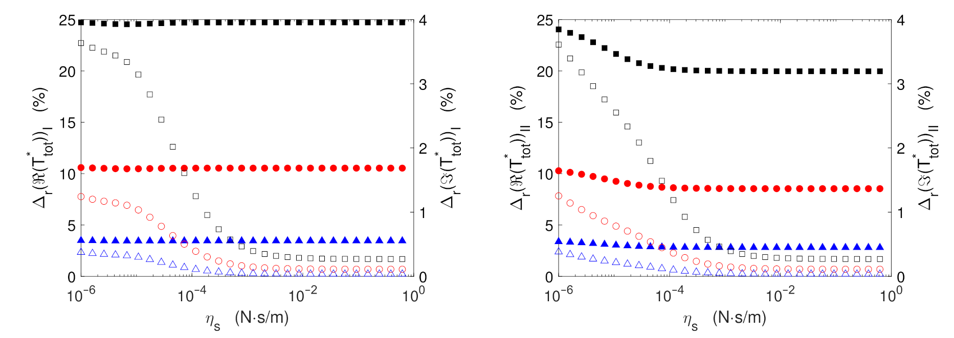
Generally speaking, both the real and imaginary parts of the relative differences in the total torque are smaller in PV-II. Moreover, for all the mesh sizes analyzed and for both versions of the numerical approach, Δ r ( ( T tot * ) ) is considerably smaller than Δ r ( ( T tot * ) ) (see the different scale of the left and right vertical axes). Interestingly, the results for PV-I show a practically constant value of the relative differences in the real part of the total torque, Δ r ( ( T tot * ) ) , while the imaginary part shows trend changes at two different values of η s . Indeed, the imaginary part levels out below η s 10 5 N·s/m and above η s 10 3 N·s/m, while showing a steep decrease in between those values upon increasing η s . On the contrary, for PV-II, the real part of the total torque is flat above η s 10 4 N·s/m and increases upon decreasing η s below that value, while the imaginary part shows a similar behavior although in this case the cross-over value is η s 10 3 N·s/m.

3.3. Complex Amplitude Ratio

The differences in the drag terms must show up in the complex amplitude ratio, A R * , too. In Figure 8, we show the relative differences in the modulus and argument of the complex amplitude ratio for the two program versions (left and right panels correspond to PV-I and PV-II, respectively). The dependence with the mesh size has been studied and the relative differences are referred to the results of the highest resolution mesh used ( 2520 × 1260 nodes). Black symbol curves correspond to a 200 × 100 mesh, red symbols to a 440 × 220 mesh, and blue symbols to a 1000 × 500 mesh. Filled and empty symbols correspond to relative differences in the modulus and argument, respectively.
The relative differences in the modulus and argument of the complex amplitude ratio show a more complex behavior as a function of η s , because the contributions of the differences in the interfacial and subphase drags are combined together with the inertia term (see Equation (9)) and nonlinearly transformed into modulus and argument.
In Figure 8, the aforementioned three distinct regions appear too. In this case the cross-over values are located approximately at η s 10 4 and η s 10 2 N·s/m. Generally speaking, the values of the relative differences for PV-II are always smaller than those corresponding to PV-I, particularly regarding the argument. Moreover, the modulus relative differences shows a monotonic variation with η s for PV-II, while this is not true for PV-I. Overall, the convergence of the results as a function of mesh size is quite good because the relative differences always decrease upon increasing mesh spatial resolution. Indeed, the relative differences between the best resolution mesh ( 2520 × 1260 nodes) and the second best resolution mesh ( 1000 × 500 nodes) are about 0.1 % in the modulus and 0.005 % in the argument. Hence, if in a given application the computing time needs to be shortened, spatial meshes of 1000 × 500 nodes or even 440 × 220 nodes might be safely used.

3.4. Local Strain at the Bicone Rim

It is not surprising that physical quantities that involve the response of the whole interface, such as the total torque, the complex amplitude ratio, or the complex interfacial viscosity, show small differences between the values obtained with both versions of the program. The opposite is true concerning physical variables that depend mostly on the local values at the bicone rim, such as the interfacial torque or the interfacial strain close to the bicone rim. The changes in the interfacial torque have already been illustrated in Figure 6. Indeed, the interfacial strain close to the bicon rim is, typically, the reference variable to study whether the measurements are made in the linear regime or not.
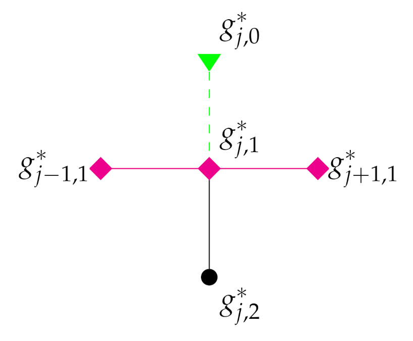
In the mathematical representation of the problem used here, the expression for the interfacial strain at the bicone rim is
γ * ( R b ) = u θ r u θ r r = R b = R b θ 0 e i ω t g * r g * r r = R b .
Hence
γ * ( R b ) θ 0 e i ω t = R b g * r r = R b g * ( R b ) = R b g * r r = R b 1 ,
and, taking into account Equation (6), the expression for the relationship between the strain at the bicone rim and the interfacial torque is
T s u r f θ 0 e i ω t = i ω 2 π R b 2 R c B o * η R b g * r r = R b 1 = i ω 2 π R b 2 R c B o * η γ * ( R b ) θ 0 e i ω t .
In Figure 9, we show the relative differences in the modulus and argument of the complex interfacial strain at the bicone rim for the two program versions (left and right panels correspond to PV-I and PV-II, respectively). The dependence with the mesh size has been studied and the relative differences are referred to the results of the highest resolution mesh used ( 2520 × 1260 nodes). Black symbol curves correspond to a 200 × 100 mesh, red symbols to a 440 × 220 mesh, and blue symbols to a 1000 × 500 mesh. Filled and empty symbols correspond to relative differences in the modulus and argument, respectively.
On the one hand, the relative differences in the modulus of the complex interfacial strain at the bicone rim, Δ r ( | γ * ( R b ) | ) , do not differ significantly for both program versions. On the other hand, the relative differences in the argument of the complex interfacial strain at the bicone rim, Δ r ( arg ( γ * ( R b ) ) ) , show large differences for η s 10 4 N·s/m. The relative differences in Δ r ( arg ( γ * ( R b ) ) ) between program versions I and II are particularly important in the range 10 5 η s 10 4 N·s/m, where the relative differences obtained with version PV-I are higher by a factor of 10 than those corresponding to version PV-II. This variation, in favor of version PV-II, is important because the range of η s between 10 5 and 10 4 N·s/m is, precisely, where more gain should be expected from using FFBDA schemes in the bicone geometry, provided the rheometer’s resolution in torque and angular displacement is good enough.

3.5. Consistency Tests

Consistency tests consist of programming a given interfacial viscosity, solving the flow field configuration, obtaining the corresponding value of the complex amplitude ratio, and feeding the data analysis scheme with those data to check if the FFBDA scheme yields the same values that were programmed initially. The test is performed for a set of 30 values of the interfacial viscosity with logarithmic spacing in the interval 10 6 η s 10 0 N·s/m. All of the results shown here have been obtained with a high resolution mesh ( 1000 × 500 nodes).
The consistency tests performed on the iterative scheme using PV-II, with the same protocol employed in [19], are shown in the left panels of Figure 10. Different rows correspond to the three aforementioned representative cases. The top row corresponds to a perfectly viscous interface, so that the real part of the complex interfacial viscosity should coincide with the programmed value of η s and the value of the imaginary part should be negligible, as it is shown in the top left panel of Figure 10, where the real part of the calculated values of the interfacial viscosity is always larger by at least three orders of magnitude than the corresponding values of the imaginary part. The middle row corresponds to a viscoelastic interface with equal real and imaginary components of the perfectly viscous interface, so that both the real and imaginary parts of the complex interfacial viscosity should coincide with the programmed value of η s . This is precisely what is shown in the middle left panel of Figure 10 where the real and imaginary parts superpose nicely in a single symbol line. The bottom row corresponds to a perfectly elastic interface, so that the real part of the complex interfacial viscosity should be negligible, while the imaginary part should coincide with the programmed value of η s . This happens again, as shown in the bottom left panel of Figure 10, but in a small region slightly above η s 10 5 N·s/m; such a behavior appeared also in PV-I [19].
The tests yielded very similar results to those reported for version I in [19]. This is not strange since in the consistency tests of each version of the software, the initial flow configuration is obtained using the same version that is used to process the data afterwards. The curves in the right side panels of Figure 10 show the number of iterations needed for convergence at each η s value for PV-II. They show very similar trends to those corresponding to PV-I [19] but the numbers of iterations needed for convergence with PV-II are slightly larger (2 to 3 more iteration steps, typically) than those corresponding to PV-I, probably a consequence of the more involved mathematical implementation of the boundary condition at the interface.

3.6. Comparative Results on Experimental Data

In the following, we illustrate the differences in the performance of both program versions on experimental data obtained in, first, thin silicone oil films of known interfacial viscosity and depth, and, second, on a pentadecanoic acid (PDA) Langmuir monolayer under an isothermal compression. All of the results shown here have been obtained with a high resolution mesh ( 1000 × 500 nodes); hence, the differences in the results obtained with program versions PV-I and PV-II have been minimized.
In Figure 11, we show the results of processing experimental data obtained at an air/water interface covered with three different silicone oil films. Red symbols: η = 33 Pa·s, d = 150 m; η s = 5 × 10 3 N·s/m. Black symbols: η = 33 Pa·s, d = 75 m; η s = 2.5 × 10 3 N·s/m. Blue symbols: η = 1 Pa·s, d = 100 m; η s = 10 4 N·s/m. In the left panel, circles and triangles correspond to the interfacial viscosity, η s ( ω ) , and interfacial loss modulus, G s ( ω ) , respectively. The values obtained with both program versions are indistinguishable in the logarithmic vertical scale chosen. Moreover, the values obtained for the interfacial viscosity agree very well with the expected value in the three cases, and the loss modulus shows a linear dependence on frequency (straight line with unity slope in the doubly logarithmic plot). Such data convergence was achieved with 5 iteration steps or less.
The corresponding relative differences in the values of the loss modulus, Δ r ( [ G s ] I , I I ) = [ G s ] I [ G s ] I I [ G s ] I I , and the interfacial viscosity, Δ r ( [ η s ] I , I I ) = [ η s ] I [ η s ] I I [ η s ] I I , processed with both versions of the program are shown in the right panel of Figure 11. As expected, the relative differences coincide for the loss modulus and the interfacial viscosity exception made of the points at which both moduli take values comparable to the resolution limit of the instrument ∼ 10 4 N/m [18], that according to the data shown in the left panel corresponds, approximately, to ω < 2 rad/s. Hence, the circles and triangles appear superposed in the right panel plot but at ω < 2 rad/s. Not surprisingly, the relative differences are much bigger for the case of the lower value of the interfacial viscosity because the case with η s = 10 4 N·s/m is close to the resolution limit of the instrument [18] and, consequently, small errors in the flow field solution yield larger errors in the determination of the values of the rheological properties. Moreover, the relative differences grow with frequency, which is not surprising because the interfacial velocity profile becomes increasingly nonlinear as the frequency is increased, and the difference between the profiles determined with both versions of the program should increase accordingly.
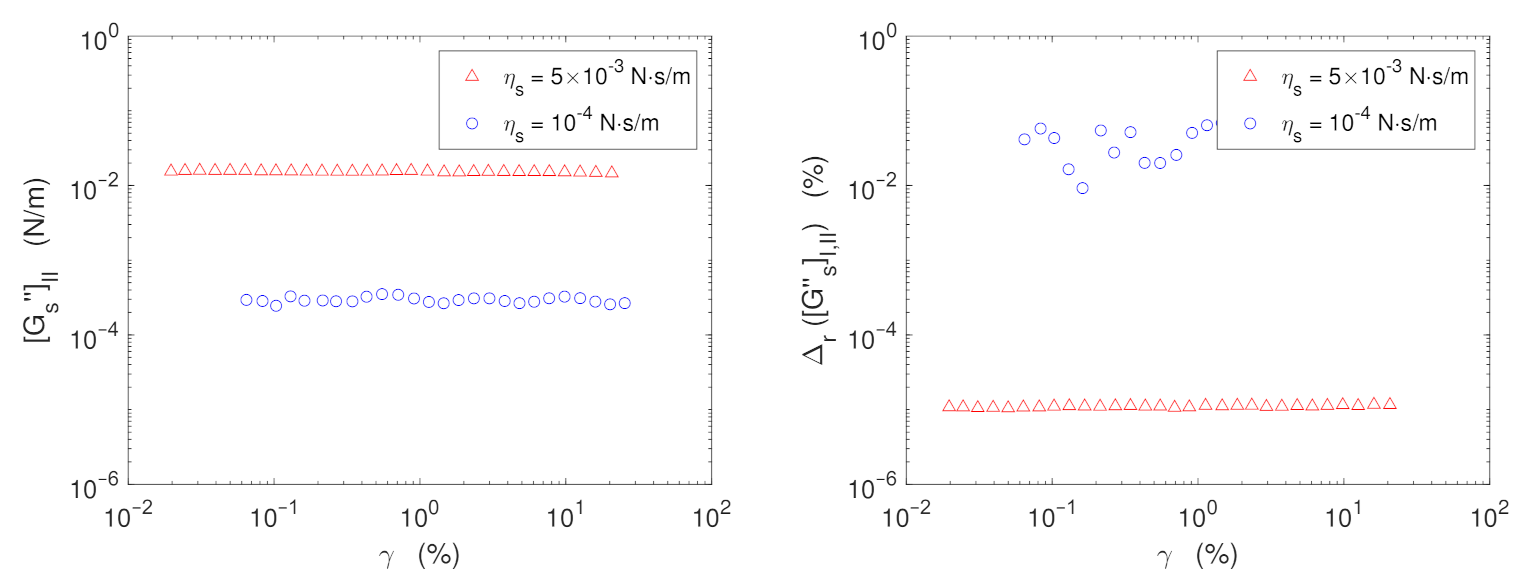
In the left panel of Figure 12, we show plots of the values obtained for the interfacial loss modulus, G s ( γ ) , as a function of the strain, γ , for the silicone oil films with η s = 5 × 10 3 N·s/m (red triangles; expected loss modulus G s 1.5 × 10 2 N/m) and η s = 10 4 N·s/m (blue circles; expected loss modulus G s 3 × 10 4 N/m)). In these measurements the frequency was set at f = 0.5 Hz ( ω = π rad/s), and the oscillation amplitude was varied. The left panel shows that the measurements are well within the linear regime, and good agreement with the expected values of the loss modulus is obtained. The corresponding relative differences in the values of the loss modulus processed with both versions of the program are shown in the right panel of Figure 12. Again, the relative differences are larger for the case of the lower value of the interfacial viscosity.
In Figure 13, we show (red triangles) the values of [ G s ] I I (red triangles) as a function of the interfacial pressure, Π , of a pentadecanoic acid Langmuir monolayer [19] obtained with PV-II, together with the relative difference, Δ r ( [ G s ] I , I I ) , between the values obtained when analyzed with both versions of the program calculated with two different mesh resolutions, namely, 1000 × 500 nodes (black dots) and 200 × 100 nodes (blue dots). From the results obtained with the high spatial resolution mesh (black dots), it is clear that the values of the difference, due to higher errors in the computations made with PV-I, are very small when the interfacial viscosity is larger than 10 3 N·s/m, roughly corresponding to interfacial pressure values above 25 mN/m, while they grow up to values about 0.1 % for lower values of the interfacial viscosity. The comparison with the results obtained using the low spatial resolution mesh (blue dots) shows that the differences increase by, roughly, a tenfold factor.

4. Conclusions

In this report, we show a detailed study of the influence of the discretization scheme close to an air/water interface in a FFBDA scheme for the bicone bob interfacial rheometer under oscillatory forcing. We have compared the performance of two program versions, using first order forward (FOFFD) and second order centered (SOCFD) finite differences discretization schemes at the interface, respectively. The SOCFD scheme needs the introduction of a line of phantom nodes above the interface. Such nodes, however, do not appear explicitly in the linear system of equations that has to be solved numerically because they are eliminated when combining the Navier–Stokes Equation (11) and the Boussinesq–Scriven boundary condition at the interface (10).
The velocity profiles at the interface show significant differences at the bicone rim, where the solutions provided by the SOCFD scheme are much smoother than those pertaining to the FOFFD one (Figure 4). Such an advantage is more noticeable the larger the nonlinearity of the profile, i.e., the lower the interfacial viscosity and the higher the oscillation frequency and the lower the spatial resolution of the mesh used in solving the hidrodynamic problem. Interestingly, the advantage in the accuracy of the flow profiles, at the highest mesh resolution used here, shows up as a few percent differences on the interface and subphase drag torques (Figure 5, Figure 6 and Figure 7), on the complex amplitude ratio (Figure 8), and on the final values obtained for the complex viscosity or dynamic moduli (Figure 10). Hence, using high resolution meshes, the values of the dynamic moduli or the complex viscosity obtained with PV-I show only marginal differences with respect to the more correct ones obtained with PV-II. Consequently, the operating windows previously reported [18] for a bicone bob ISR supplemented with BiconeDrag PV-I should be valid too when using PV-II. Regarding the computation time, PV-II requires, typically, only about 20 % more iteration steps than PV-I to achieve convergence. Such an increase in time cost is not relevant for the typical applications of the program.

Author Contributions

All authors have contributed equally to this work. All authors have read and agreed to the published version of the manuscript.

Funding

The authors acknowledge partial support from MINECO (Grant No. FIS2017-86007-C3-3-P). P.S.P. acknowledges the Programa Operativo Empleo Juvenil, co-funded by the Fondo Social Europeo and the Ministerio de Ciencia e Innovación (MICINN) and UNED for the funding of the contract with reference No. PEJ2018-005480-A.

Data Availability Statement

Not applicable.

Acknowledgments

The authors acknowledge technical and administrative support by M.J. Retuerce.

Conflicts of Interest

The authors declare no conflict of interest.

Abbreviations

The following abbreviations are used in this manuscript:
FFBDAFlow field-based data analysis
FOFFDFirst order forward finite differences
SOCFDSecond order centered finite differences
DWRDouble wall-ring
ISRInterfacial shear rheometer
PV-IProgram version I
PV-IIProgram version II
PDAPentadecanoic acid

References

  1. Harkins, W.D.; Kirkwood, J.G. The Viscosity of Monolayers: Theory of the Surface Slit Viscosimeter. J. Chem. Phys. 1938, 6, 53. [Google Scholar] [CrossRef]
  2. Harkins, W.D.; Kirkwood, J.G. Note on Surface Viscosimetry. J. Chem. Phys. 1938, 6, 298. [Google Scholar] [CrossRef]
  3. Nutting, G.C.; Harkins, W.D. The Viscosity of Monolayers: A Test of the Canal Viscosimeter. J. Am. Chem. Soc. 1940, 62, 3155–3161. [Google Scholar] [CrossRef]
  4. Myers, R.J.; Harkins, W.D. The Viscosity (or Fluidity) of Liquid or Plastic Monomolecular Films. J. Chem. Phys. 1937, 5, 601–603. [Google Scholar] [CrossRef]
  5. Dervichian, D.; Joly, M. Transformations d’ordre supérieur dans les couches monomoléculaires. J. Phys. Radium 1939, 10, 375–384. [Google Scholar] [CrossRef]
  6. Sánchez-Puga, P.; Tajuelo, J.; Pastor, J.M.; Rubio, M.A. Flow field-based data analysis in interfacial shear rheometry. Adv. Colloid Interface Sci. 2021, 288, 102332. [Google Scholar] [CrossRef]
  7. Reynaert, S.; Brooks, C.F.; Moldenaers, P.; Vermant, J.; Fuller, G.G. Analysis of the magnetic rod interfacial stress rheometer. J. Rheol. 2008, 52, 261–285. [Google Scholar] [CrossRef] [Green Version]
  8. Vandebril, S.; Franck, A.; Fuller, G.G.; Moldenaers, P.; Vermant, J. A double wall-ring geometry for interfacial shear rheometry. Rheol. Acta 2010, 49, 131–144. [Google Scholar] [CrossRef]
  9. Verwijlen, T.; Moldenaers, P.; Stone, H.A.; Vermant, J. Study of the Flow Field in the Magnetic Rod Interfacial Stress Rheometer. Langmuir 2011, 27, 9345–9358. [Google Scholar] [CrossRef]
  10. Tajuelo, J.; Pastor, J.M.; Martínez-Pedrero, F.; Vázquez, M.; Ortega, F.; Rubio, R.G.; Rubio, M.A. Magnetic Microwire Probes for the Magnetic Rod Interfacial Stress Rheometer. Langmuir 2015, 31, 1410–1420. [Google Scholar] [CrossRef]
  11. Tajuelo, J.; Pastor, J.M.; Rubio, M.A. A magnetic rod interfacial shear rheometer driven by a mobile magnetic trap. J. Rheol. 2016, 60, 1095–1113. [Google Scholar] [CrossRef]
  12. Renggli, D.; Alicke, A.; Ewoldt, R.H.; Vermant, J. Operating windows for oscillatory interfacial shear rheology. J. Rheol. 2020, 64, 141–160. [Google Scholar] [CrossRef] [Green Version]
  13. Soo-Gun, O.; Slattery, J.C. Disk and biconical interfacial viscometers. J. Colloid Interface Sci. 1978, 67, 516–525. [Google Scholar] [CrossRef]
  14. Erni, P.; Fischer, P.; Windhab, E.J.; Kusnezov, V.; Stettin, H.; Läuger, J. Stress- and strain-controlled measurements of interfacial shear viscosity and viscoelasticity at liquid/liquid and gas/liquid interfaces. Rev. Sci. Instruments 2003, 74, 4916–4924. [Google Scholar] [CrossRef]
  15. Miller, R.; Liggieri, L. Interfacial Rheology; Progress in Colloid and Interface Science; CRC Press: Boca Raton, FL, USA, 2009. [Google Scholar]
  16. Krägel, J. Surface shear rheology. In Interfacial Rheology; Miller, R., Liggieri, L., Eds.; CRC Press: New York, NY, USA, 2009; Volume 1. [Google Scholar]
  17. Tajuelo, J.; Rubio, M.A.; Pastor, J.M. Flow field based data processing for the oscillating conical bob interfacial shear rheometer. J. Rheol. 2017, 62, 295–311. [Google Scholar] [CrossRef]
  18. Sánchez-Puga, P.; Tajuelo, J.; Pastor, J.; Rubio, M.A. Dynamic Measurements with the Bicone Interfacial Shear Rheometer: Numerical Bench-Marking of Flow Field-Based Data Processing. Colloids Interfaces 2018, 2, 69. [Google Scholar] [CrossRef] [Green Version]
  19. Sánchez-Puga, P.; Tajuelo, J.; Pastor, J.M.; Rubio, M.A. BiconeDrag—A data processing application for the oscillating conical bob interfacial shear rheometer. Comput. Phys. Commun. 2019, 239, 184–196. [Google Scholar] [CrossRef] [Green Version]
  20. Sanchez-Puga, P.; Tajuelo, J.; Pastor, J.M.; Rubio, M.A. BiconeDrag—A data processing application for the oscillating conical bob interfacial shear rheometer. Mendeley Data (MATLAB Pyhton3 Codes) 2018. [Google Scholar] [CrossRef] [Green Version]
  21. Guzmán, E.; Tajuelo, J.; Pastor, J.M.; Rubio, M.A.; Ortega, F.; Rubio, R.G. Shear rheology of fluid interfaces: Closing the gap between macro- and micro-rheology. Curr. Opin. Colloid Interface Sci. 2018, 37, 33–48. [Google Scholar] [CrossRef]
  22. Sánchez-Puga, P.; Tajuelo, J.; Pastor, J.; Rubio, M.A. BiconeDrag Updated—A data processing application for the oscillating conical bob interfacial shear rheometer. Comput. Phys. Commun. 2021. to appear. [Google Scholar]
  23. Sanchez-Puga, P.; Tajuelo, J.; Pastor, J.M.; Rubio, M.A. BiconeDrag II—A data processing application for the oscillating conical bob interfacial shear rheometer. Code Ocean (MATLAB Code) 2021. [Google Scholar] [CrossRef]
  24. Sanchez-Puga, P.; Tajuelo, J.; Pastor, J.M.; Rubio, M.A. BiconeDrag II—A data processing application for the oscillating conical bob interfacial shear rheometer. Mendeley Data (MATLAB Python3 Codes) 2021. to appear. [Google Scholar] [CrossRef]
  25. Scriven, L. Dynamics of a fluid interface Equation of motion for Newtonian surface fluids. Chem. Eng. Sci. 1960, 12, 98–108. [Google Scholar] [CrossRef]
  26. Fitzgibbon, S.; Shaqfeh, E.S.G.; Fuller, G.G.; Walker, T.W. Scaling analysis and mathematical theory of the interfacial stress rheometer. J. Rheol. 2014, 58, 999–1038. [Google Scholar] [CrossRef]
Figure 1. Sketch of the new mesh. Blue up triangles: nodes at the cylindrical symmetry axis inside the subphase. Red dots: nodes at the bottom wall of the cup. Grey squares: nodes at the bicone surface. Black dots: nodes inside the fluid subphase. Black crosses: nodes at the outer cup wall. Magenta diamonds: nodes at the interface. Green down triangles: phantom nodes above the interface.
Colloids 05 00017 g001
Figure 2. Four node scheme at the interface. Black dot: node inside the fluid subphase. Magenta diamonds: nodes at the interface. Green down triangle: phantom node above the interface.
Colloids 05 00017 g002
Figure 3. Color coded plot of [ g I I * ( r , z ) ] [ g I * ( r , z ) ] (left) and [ g I I * ( r , z ) ] [ g I * ( r , z ) ] (right) for a viscoelastic interface with B o * = 0.1 0.1 i , at ω = π rad/s. The highest value of the velocity field amplitude is 1 just at the bicone rim.
Colloids 05 00017 g003
Figure 4. Real and imaginary parts of g s , I * ( r ) (left) and g s , I I * ( r ) (right) for ω and B o * values as in Figure 3. Top row: 440 × 220 mesh. Bottom row: 2520 × 1260 . Continuous and dashed lines represent the real and imaginary parts, respectively. Case A: High frequency with a viscoelastic interface (black). Case B: Medium frequency with purely viscous interface (red). Case C: Low frequency and clean air–water interface (blue).
Colloids 05 00017 g004
Figure 5. Subphase drag torque relative differences between the solutions with different mesh sizes taking as a reference the 2520 × 1260 mesh solution for the real part, Δ r ( ( T sub * ) ) (solid symbols), and the imaginary part, Δ r ( ( T sub * ) ) (open symbols). Black symbols: 200 × 100 mesh. Red symbols: 440 × 220 mesh. Blue symbols: 1000 × 500 . Left panel: program version (PV)-I, right panel: PV-II.
Colloids 05 00017 g005
Figure 6. Interfacial drag torque relative differences between the solutions with different mesh sizes taking as a reference the 2520 × 1260 mesh solution for the real part, Δ r ( ( T surf * ) ) (solid symbols), and the imaginary part, Δ r ( ( T surf * ) ) (open symbols). Black symbols: 200 × 100 mesh. Red symbols: 440 × 220 mesh. Blue symbols: 1000 × 500 . Left panel: PV-I, right panel: PV-II.
Colloids 05 00017 g006
Figure 7. Total drag force relative differences between the solutions with different mesh sizes taking as a reference the 2520 × 1260 mesh solution for the real part, Δ r ( ( T tot * ) ) (solid symbols), and the imaginary part, Δ r ( ( T tot * ) ) (open symbols). Black symbols: 200 × 100 mesh. Red symbols: 440 × 220 mesh. Blue symbols: 1000 × 500 . Left panel: PV-I, right panel: PV-II.
Colloids 05 00017 g007
Figure 8. Relative differences in modulus, Δ r ( A R ) (solid symbols), and phase, Δ r ( a r g ) (open symbols), between the solutions obtained with different mesh sizes taking as a reference the 2520 × 1260 mesh solution. Black symbols: 200 × 100 mesh. Red symbols: 440 × 220 mesh. Blue symbols: 1000 × 500 . Left panel: PV-I; right panel: PV-II.
Colloids 05 00017 g008
Figure 9. Relative differences in the modulus, Δ r ( | γ * ( R b ) | ) (solid symbols), and the argument, Δ r ( arg ( γ * ( R b ) ) ) (open symbols), of the interfacial strain at the bicone rim between the solutions obtained with different mesh sizes taking as a reference the 2520 × 1260 mesh solution. Black symbols: 200 × 100 mesh. Red symbols: 440 × 220 mesh. Blue symbols: 1000 × 500 . Left panel: PV-I; right panel: PV-II.
Colloids 05 00017 g009
Figure 10. Real (solid circles) and imaginary (open circles) parts of the interfacial shear viscosity (left column) and number of iterations (triangles) until convergence (right column) as a function of the interfacial shear viscosity modulus, | η s * | at a frequency f = 0.5 Hz. Upper row: Purely viscous interface ( η s = 0 ). Middle row: Viscoelastic interface ( η s = η s ). Bottom row: Purely elastic interface ( η s = 0 ).
Colloids 05 00017 g010
Figure 11. Left panel: Interfacial loss modulus, [ G s ] I I (triangles), and interfacial viscosity, η s (circles) as a function of oscillation frequency, ω . Right panel: Relative difference, Δ r ( [ G s ] I , I I ) , between the loss modulus of the thin films of silicone oil obtained with PV-I and PV-II as a function of frequency.
Colloids 05 00017 g011
Figure 12. Left panel: Interfacial loss modulus, [ G s ] I I as a function of strain, γ , for the silicone oil films with η s = 5 × 10 3 N·s/m (red triangles) and η s = 10 4 N·s/m (blue circles). Right panel: Relative difference, Δ r ( [ G s ] I , I I ) , between the loss modulus of the thin films of silicone oil obtained with PV-I and PV-II as a function of strain.
Colloids 05 00017 g012
Figure 13. Loss modulus, [ G s ] I I , (red triangles) and relative difference, Δ r ( [ G s ] I , I I ) , between results using PV-I and PV-II (black dots) of a PDA Langmuir monolayer, as a function of the interfacial pressure Π . The relative differences Δ r ( [ G s ] I , I I ) are shown for two different spatial resolution meshes: 1000 × 500 nodes (black dots) and 200 × 100 nodes (blue dots).
Colloids 05 00017 g013
Publisher’s Note: MDPI stays neutral with regard to jurisdictional claims in published maps and institutional affiliations.

