Holocene Carbon Burial in Lakes of the Uinta Mountains, Utah, USA


Geology Department, Middlebury College, Middlebury, VT 05753, USA
*
Author to whom correspondence should be addressed.
Quaternary 2019, 2(1), 13; https://0-doi-org.brum.beds.ac.uk/10.3390/quat2010013
Submission received: 22 February 2019
/
Revised: 8 March 2019
/
Accepted: 13 March 2019
/
Published: 16 March 2019
Abstract
:Recent research suggests that organic matter sequestered in lake sediment comprises a larger component of the global carbon cycle than once thought, yet little is known about carbon storage in mountain lakes. Here, we used a set of sediment cores collected from lakes in the Uinta Mountains (Utah, USA) to inform a series of calculations and extrapolations leading to estimates of carbon accumulation rates and total lacustrine carbon storage in this mountain range. Holocene rates of carbon accumulation in Uinta lakes are between 0.1 and 20.5 g/m2/yr, with an average of 5.4 g/m2/yr. These rates are similar to those reported for lakes in Greenland and Finland and are substantially lower than estimates for lakes in Alberta and Minnesota. The carbon content of modern sediments of seven lakes is notably elevated above long-term Holocene values, suggesting recent changes in productivity. The lakes of the Uintas have accumulated from 6 to 10 × 105 Mt of carbon over the Holocene. This is roughly equivalent to the annual carbon emissions from Salt Lake City, Utah. Based on their long-term Holocene rates, lakes in the Uintas annually sequester an amount of carbon equivalent to the emissions of <20 average Americans.
1. Introduction
Lakes cover <4% of the Earth’s non-glaciated land surface [1], yet they play an outsized role in the carbon cycle [2,3,4]. Lakes are sites of autochthonous organic matter production and locations where both autochthonous lacustrine and allochthonous terrestrial organic carbon are deposited [3]. In the first years after deposition, some of this organic matter is mineralized to CO2 and CH4 and is lost through water outflow and degassing at the surface [5]. However, the majority of this material escapes conversion due to of a lack of dissolved oxygen in some deep lake waters, and because high rates of sedimentation quickly bury organic matter, isolating it from the water column [5]. As a result, this organic matter is essentially removed from the carbon cycle for millennia [2,6].
Given the significant role of lakes in the global carbon cycle, two obvious questions are “how much carbon is stored in modern lake sediments?” and “how much carbon is removed from the atmosphere each year by sedimentation in lake basins?” In pursuit of answers to these questions, considerable effort has focused on quantifying carbon stored in lakes [5,7]. Much of this work has followed two different approaches. The first is to use a relatively small number (<~20) of Holocene-length lake sediment cores as grounds for extrapolation to the landscape scale [8,9,10,11]. These studies typically benefit from a deeper-time perspective provided by long sedimentary records, and cores can be combined with sub-bottom profiling to more accurately estimate sediment volumes [7,11]. On the other hand, these studies are typically hampered by assumptions made during analysis of the sediment. For instance, loss-on-ignition is often measured as a proxy for carbon content [12], rather than directly measuring carbon with an elemental analyzer, which is time consuming and more expensive. Large numbers of long cores are also rarely analyzed at cm-scales due to the huge number of samples involved. Bulk density values are also required to convert carbon content in percent to carbon content by mass. Yet because bulk density can be difficult to measure, it is often estimated from sediment organic content [10], introducing the potential for circularity.
A completely different approach is to calculate modern rates of carbon sequestration from recently deposited lake sediments [13,14,15]. Studies employing this method often involve much larger numbers of lakes (>100), yet because they focus solely on recent sediments, they cannot resolve long-term rates of carbon accumulation. There are also indications that modern rates of carbon accumulation are not representative of pre-Anthropocene rates [16], which undermines attempts to use modern rates to estimate carbon stores. Nonetheless, recent estimates of annual global carbon sequestration in inland waters range from 0.06 to 0.25 Pg/yr [15], considerably greater than an earlier estimate of 0.04 Pg/yr [17], and similar to the annual global oceanic sediments carbon sink of 0.12 Pg/yr [18].
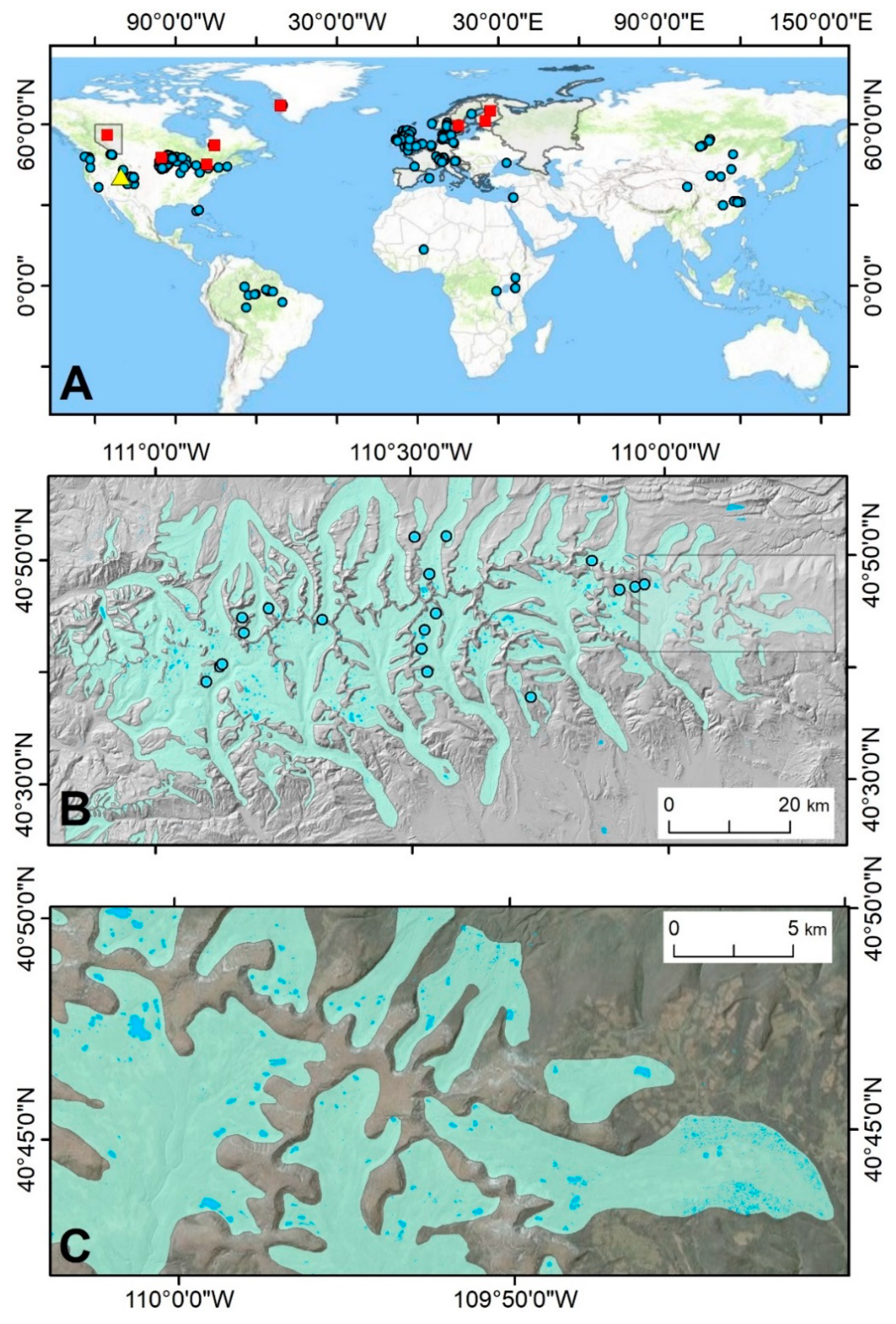
Furthermore, regardless of whether studies have utilized long cores or focused on modern sediments, there are significant issues related to the over-representation of large lakes in these compilations and the uneven distribution of studied lakes on the landscape. For instance, despite the fact that small lakes may sequester more carbon per area than larger water bodies [2,4,8], many studies of lacustrine carbon storage are dominated by relatively large lakes [6]. At the same time, not all biomes are equally represented in these compilations. For instance, the first estimate of the global lacustrine carbon sink started with just three lake cores from Minnesota (USA) before expanding to predict total carbon sequestration in all the world’s inland waters [17]. In subsequent work, the majority of carbon storage estimates extrapolated from long cores have focused on boreal and arctic landscapes [7,8,9,10,11,19,20,21]. Similarly, even the most comprehensive compilations of carbon in modern sediments still exhibit pronounced clustering (Figure 1A), with an over-representation of sites in northeastern North America and Europe [14,15]. As a result, there are no organic carbon burial measurements available for 85% of the world’s major catchments [15]. Overall, while extensive progress has been made in understanding the role of boreal and arctic lakes as sites of long-term carbon storage, little attention has been paid to lakes in other biomes, and the role of small lakes has typically been overlooked.
Mountain landscapes, particularly those that were subject to glaciation during the Pleistocene, often feature abundant lakes in basins produced by glacial erosion and deposition. However, lakes in mountain settings constitute a distinct minority of the sites used to compile modern rates of lacustrine carbon sequestration (Figure 1A) [14,15]. Furthermore, although some studies have reported bulk density and carbon contents for Holocene-length records from mountain lakes [22] these have typically been isolated projects focused on individual lakes that were not intended or used to yield broader estimates of lacustrine carbon in mountain settings.
To address this data gap, this study focused explicitly on a lake-rich landscape in part of the US Rocky Mountains (Figure 1A). Sediment analysis was combined with multiple linear regression, extrapolation, and geospatial analysis in a geographic information system (GIS) to answer three related questions:
- What is the Holocene-scale rate of carbon storage in lakes of this study area?
- How does this long-term average rate compare with modern values?
- How much carbon is stored in these lakes?
2. Materials and Methods
2.1. Study Area
The lakes cored in this project are located in the Uinta Mountains (hereafter, the “Uintas”), a component of the Rocky Mountain system in the western United States (Figure 1). Geologically the Uintas are a ~7 km-thick sequence of Precambrian quartzite, sandstone and argillite that was uplifted during the Laramide Orogeny forming a mountain range ~200 km long [23,24,25]. Summit elevations in the central part of the Uintas are >4 km above sea level (asl) and treeline is at an elevation of ~3.3 km asl. Although the Uintas are not currently glacierized, classic alpine glacial geomorphology records the presence of >2000 km2 of glacial ice during the Last Glacial Maximum [26]. These glaciers began to retreat around 18,000 years ago [27,28], leaving behind a landscape characterized by a huge number of lakes (Figure 1B, 1C) [29,30]. Representative Uinta lakes investigated in a previous study were classified as oligotrophic to oligo-mesotrophic on the basis of total phosphorus, total nitrogen, chlorophyll α, and Secchi depth values [31]. Depending on their elevation, Uinta lakes are surrounded by a variety of vegetation communities [32,33]. Alpine landscapes are mantled by tundra featuring abundant forbs including Acomastylis rossii (Alpine avens) and Polygonum bistortoides (alpine bistort). Picea engelmannii (Engelmann spruce) and Abies lasiocarpa (subalpine fir) dominate the upper-subalpine forests, giving way at intermediate elevations to a monoculture of Pinus contorta (lodgepole pine). Lakes in forest openings are bordered by meadows with common species including Danthonia intermedia (wild oat grass), Deschampsia caespitosa (tufted hairgrass), and Carex scirpodiea (single spike sedge) [33]. The climate of the Uintas is characterized by long, snowy winters and relatively cool summers. Mean annual precipitation ranges from 500 to 925 mm, decreasing eastward, with more than 60% falling as snow at elevations >3.3 km asl [34,35]. The mean annual temperature above ~3.1 km asl is <0°C [36,37,38]. Under these conditions, lakes freeze over in the winter, with a duration of ice cover extending roughly from October through June.
2.2. Field Methods
In the course of a project focused on post-glacial environmental change (Munroe, GSA Bulletin, in press), multiple lakes in the Uinta Mountains were cored from a floating platform; 19 of those cores are considered here (Table 1). Prior to coring, a bathymetric survey was conducted with a GPS- enabled sonar device, and the perimeter of each lake was explored on foot. Information from this survey was used to select a coring location in deep water near the lake center, far from prominent inlets or steep slopes (terrestrial and subaqueous) that could deliver sediment through mass wasting. A modified Reasoner-type percussion corer [39] fitted with a piston, metal nose cone with integrated core catcher, and ~30 kg driving weight was used to collect sediment in a 6 m-long barrel of 7.5 cm diameter PVC pipe. Driving of the percussion corer began at the sediment-water interface, but it was not possible to retrieve the unconsolidated near-surface sediment with this technique. As a result, all percussion cores were artificially truncated at a depth of ~50 cm. After driving to the point of refusal, the core barrels were extracted with a winch. Cores were cut to ~80 cm lengths with a hacksaw, capped, and transported by pack animals before shipping. In seven lakes selected for their ease-of-access, near-surface sediments (<50 cm) were collected using a UWITEC gravity corer. No attempt was made to correlate these gravity cores with the percussion cores because the amount of overlap between them, if any, was unknown. These cores were extruded on the lakeshore, and 2 cm-thick subsamples of the top, middle, and the bottom of each core were collected. After arrival in the lab, all percussion core sections and gravity core subsamples were stored at 4 °C until processing.
2.3. Analytical Methods
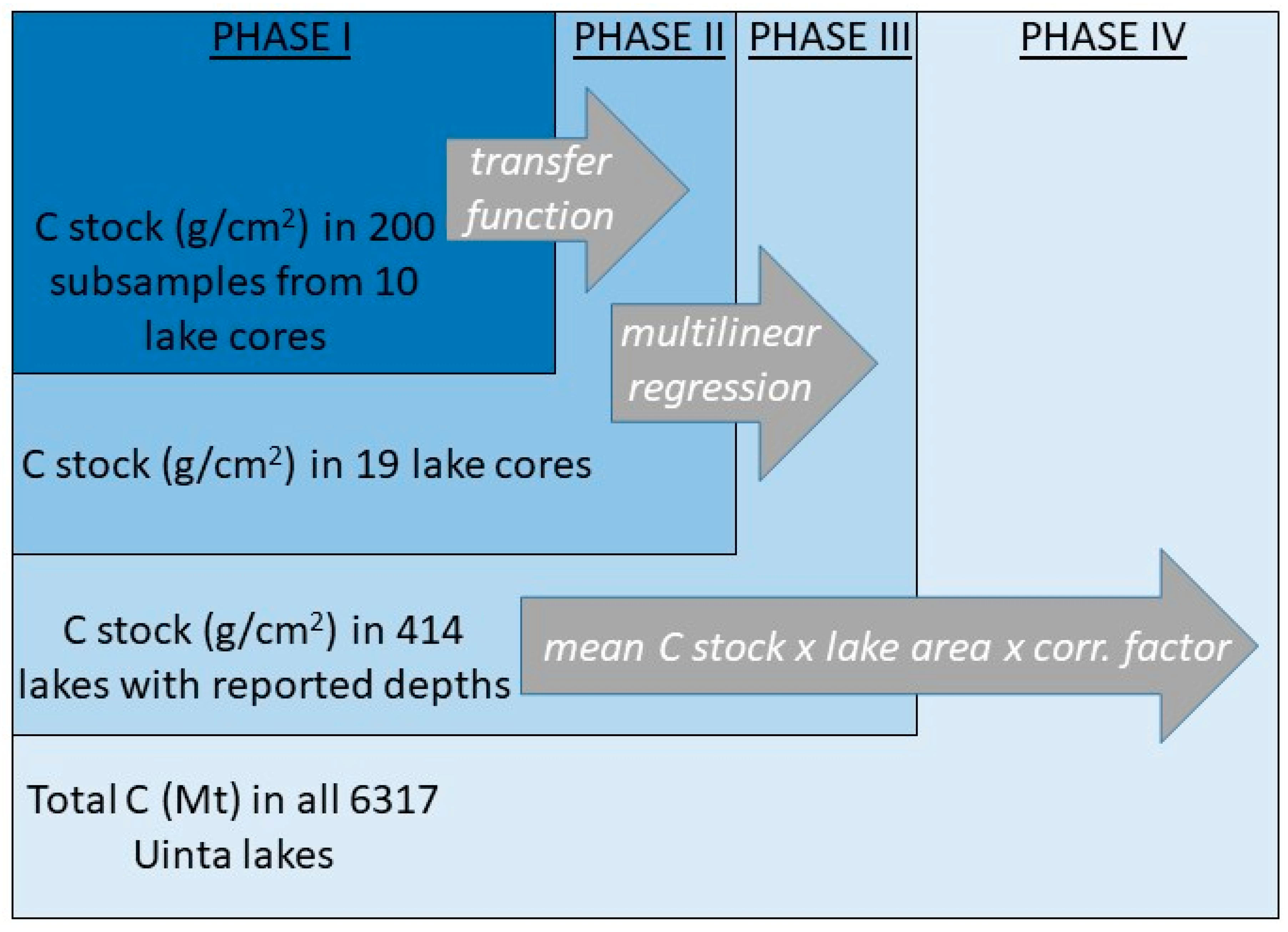
This study employed a series of sequential extrapolations to proceed from measurements made on the collected lake sediment cores, to a range-wide estimate of carbon accumulation rates and storage in all Uinta Mountain lakes. This approach is presented graphically in Figure 2. Briefly, in Phase I, bulk density and water content were measured for a random subset of samples and a regression between these variables was developed. In Phase II, this regression was employed as a transfer function to convert water content measurements for all cores into estimates of bulk density. These were then combined with measurements of carbon abundance to calculate total carbon content in each of the cores. In Phase III, multilinear regression was used to identify which variables describing the dimensions and physical setting of each lake were the best predictors for each lake’s carbon pool. This relationship supported estimates of carbon storage in the lakes for which depth data are available. Finally, in Phase IV, estimates of carbon storage in these lakes were then combined with lake areas to yield the total carbon stored in all lakes in the Uintas. Details of these procedures are presented in the following subsections.
2.3.1. Phase I: Measuring Water and C Content, Estimating Bulk Density
Percussion cores from 19 Uinta Mountain lakes were subsampled in quadruplicate at 1 cm resolution. As part of a project developing records of post-glacial environmental change from these cores (Munroe, GSA Bulletin, in press), one of these samples was consumed in a Leco TGA-701 thermogravimetric analyzer (TGA) to determine water content and loss-on-ignition. A second subsample was freeze-dried, ground, and analyzed in a Thermo Flash 2000 Elemental Analyzer to determine carbon and nitrogen content. The third subsample was consumed for analysis of grain size distribution, and the fourth was retained as an archive. Loss-on-ignition and grain size results are not presented here. Radiocarbon dates were generated for these cores, primarily on terrestrial macrofossils including conifer needles and cones, small wood fragments and twigs, and macroscopic charcoal. Radiocarbon results were calibrated with the Intcal13 calibration curve [40] and used along with their stratigraphic depths to construct depth-age models in the program CLAM [41]. Details of these procedures are presented in Munroe (GSA Bulletin, in press).
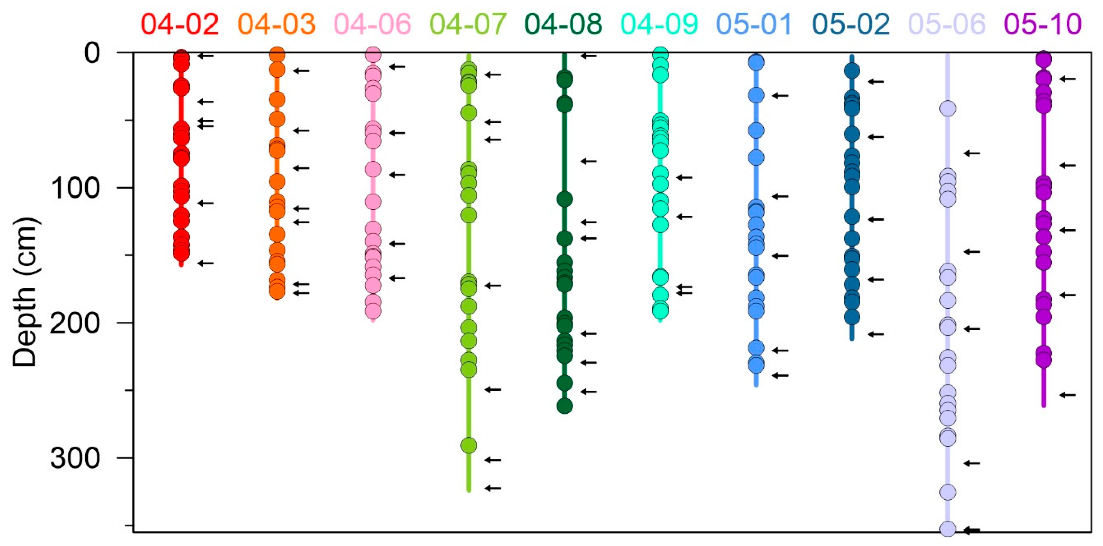
For the carbon study reported here, ten lake cores—representing a variety of landscape positions and lake dimensions, and with complete sets of archived samples from top to bottom—were selected for direct evaluation of bulk density. A random number generator was used to select 20 samples from each of these cores (Figure 3). The volume of these samples was measured with a Pentapyc 5200e pycnometer. The samples were then freeze-dried and weighed, and the combination of wet volume and dry mass was used to calculate bulk density (g/cm3).
These direct bulk density measurements were used to establish a relationship between sediment water content and bulk density. First, 17 samples identified as outliers were removed to produce a trimmed dataset. All of these had volumes <1 cm3, which apparently contributed to spurious results when they were measured in the pycnometer. Second, to evaluate whether water content could effectively predict bulk density, the trimmed dataset was randomly split in half. A regression relating moisture content and bulk density was then developed for one half of the data and used to predict the other half. These predicted values were compared with the measured values to demonstrate the strength of the regression as a transfer function. This analysis was conducted twice, with different random splits of the data. After confirming that bulk density could be predicted reliably from water content, a regression between the two variables was calculated for the full trimmed dataset.
2.3.2. Phase II: Estimation of the Holocene Carbon Accumulation Rate and Carbon Stock
The transfer function developed in Phase I was used to estimate bulk density through all of the Uinta cores using the water contents previously measured with the TGA (Figure 2). This procedure produced values of estimated bulk density at 1 cm spacing through the 10 cores from which the bulk density subsamples were taken, as well as the nine cores for which bulk density was not directly measured. Multiplying these estimated bulk density measurements by the percent carbon in each sample determined by the elemental analyzer yielded the mass of carbon per sample. Summing these masses for all of the samples in a given core yielded an estimated of the carbon in that core (normalized to 1 cm2 of lake bottom). Although many of these cores extend back into the late Pleistocene [42], only sediment that accumulated after 11,700 BP was included in this sum to constrain this analysis to the Holocene. Furthermore, because the upper parts of each core were artificially truncated by the percussion coring technique, carbon sums were calculated up to a depth in each core corresponding to 2000 BP, the age of the oldest core top. This carbon total for each core (between 11,700 and 2000 BP) was divided by 9700 to yield an average carbon accumulation rate (g/cm2/yr). This value was then multiplied by 11,700 years to estimate the amount of carbon that accumulated in the Holocene (hereafter the “carbon stock” in g/cm2). These results are presented in Table S1.
2.3.3. Phase III: Extrapolating Using Spatial Predictors
The Uinta Mountains contain many more lakes than could be cored, so extrapolation was required to generate range-wide estimates of carbon storage. This goal was met through a GIS analysis that measured spatial variables describing the dimensions and settings of these lakes, and a statistical analysis that revealed which of these variables are valid predictors of each lake’s carbon stock (Figure 2).
A database representing the digital outlines of the lakes in Utah was downloaded from the National Hydrography Dataset (Figure 1B). These data were projected in UTM Zone 12N (NAD83) with a vertical datum of NAVD88. Because nearly all of the natural lakes in the Uintas are located within areas impacted by glacial erosion and deposition during the Pleistocene, the downloaded lake database was clipped with the reconstructed outlines of alpine glaciers in the Uintas at the Last Glacial Maximum [26]. The resulting dataset was further processed to remove polygons coded as marsh, swamp, or intermittent water, leaving only perennial water bodies. The area and perimeter of the polygon representing each lake were calculated, along with complexity (perimeter of each lake divided by the perimeter of a circle with the same area as the lake). The polygons were then sorted by area from largest to smallest, and seven large artificial reservoirs were deleted. The lack of an original lake at these locations was confirmed by comparison with a 1909 map of the Uintas [30]. Centroids were then determined for each lake polygon, and the elevation of each centroid was calculated from a 10 m digital elevation model (DEM).
A variety of automated watershed delineation methods was explored, but unfortunately all failed to generate realistic watersheds in this complex landscape with abundant, closely spaced water bodies. As an alternate approach, a 100 m wide buffer was determined around the perimeter of each lake. These buffers were converted to a raster and each cell was assigned the value of the corresponding lake elevation. This raster buffer layer was divided by the DEM layer, so that cells at elevations at or above the lake had values of one or greater; cells with values <1 were reclassified to “NoData.” The raster was then converted back into a polygon layer delineating the “uphill buffer”: land area within 100 m of each lake with an elevation above that lake surface.
Two additional analyses were conducted to characterize the area within the uphill buffer associated with each lake. First, a slope raster was generated from the DEM, and zonal statistics were used to calculate average slope and slope range within each uphill buffer. Second, a Landsat 8 image from 10 August, 2018 was classified into five spectrally distinct landcover types: Bare ground, forest, water, biocrust/tundra, and agriculture. The area of each cover type within the uphill buffer of each lake was then tabulated.
Depths for ~500 lakes in the Uintas have been reported by the Utah Division of Wildlife Resources. Values for 414 lakes were manually appended to the lake dataset in the GIS. Most lakes for which depth values were not entered are small and unnamed and it was not possible to cross-reference them with the GIS.
Upon inspection of the carbon results for the cored Uinta lakes, three outlier cores were identified. The cores from two lakes (05-05 and 05-07) did not span the entire Holocene, thus it was deemed inappropriate to extrapolate their average sedimentation rates to the time period matching the other lakes (Table 1). A third lake (05-08) is singularly impacted by cold, turbid inflow from adjacent rock glaciers [43]. As a result, its carbon content is an outlier when compared with the other lakes.
The remaining 16 lakes were used to build a multilinear regression with Holocene carbon stock (in g/cm2 of lake bottom) as the target variable (Figure 2). The analysis was conducted in SPSS v.25 with ten variables as possible predictors. Six of these pertained to the lake itself: Perimeter, elevation, depth, area/depth ratio, area (log10), and complexity (log10). Four of these pertained to the uphill buffer around each lake: Percent bare ground, percent forest cover, mean slope, and range of slope. The analysis utilized forward stepwise construction, and the adjusted r2 was employed as the criterion for including predictors. The resulting regression was then used to estimate the carbon stock (in g/cm2) in the 414 lakes for which depth data were available. These results are presented in Table S2.
2.3.4. Phase IV: Extrapolating to Landscape Scale
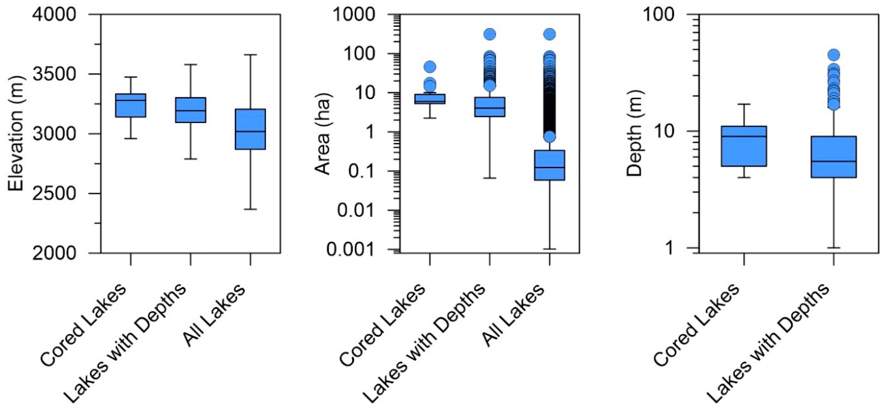
Estimates of carbon stock in all lakes of the Uintas (n = 6317) were made using six different “average” values: (1) Median and (2) mean carbon stock in the 19 cored lakes, (3) the mean for the smallest 25% of cored lakes, (4) median and (5) mean carbon stock predicted from the multilinear regression, and (6) the mean of the values predicted by the multilinear regression for the smallest 25% of the lakes. The smallest 25% threshold was used because the cored lakes and the lakes with reported depths are larger than the average Uinta lake (Figure 4).
These six estimates of carbon stock (g/cm2) in all Uinta lakes were multiplied by the area of each lake and divided by four to produce an estimate of each lake’s Holocene carbon pool. These results are presented in Table S3. This extrapolation is obviously vulnerable to possible sediment focusing [44] and the reality that sediment thickness and properties vary laterally within a lake basin [7,11]. Previous work has revealed that lake carbon pool estimates calculated by extrapolating a single depocenter core to the entire lake area are up to four times too large in comparison with sediment volume calculations made with a sub-bottom profiler [11]. Because depth data are not available for all Uinta lakes, because sub-bottom profiling was beyond the scope of this study, and because the number of lakes involved in this range-wide inventory is large, extrapolation was necessary, and the resulting uncertainty is an unfortunate reality. The use of six different estimates of average carbon stock, as well as the division step to correct sediment volume, are intended to help mitigate this inevitable uncertainty.
3. Results
3.1. Phase I: Measuring Water and C Content, Estimating Bulk Density
As part of a previous project (Munroe, GSA Bulletin, in press), measurements of water content were made for 4641 samples from 19 Uinta lake cores using the TGA. Percent carbon and nitrogen were measured with an elemental analyzer for 4619 samples. This total is lower because values were below detection limits in some deep, inorganic sediments (Table 1)
Bulk densities measured with the pycnometer ranged from 0.058 to 2.33 g/cm3 with a mean of 0.54 g/cm3, a median of 0.43 g/cm3, and a skewness of 2.47. After removal of the low-volume samples that yielded spurious results, the mean is 0.52 g/cm3 (±0.37), the median 0.42 g/cm3, and the skewness 2.8. The 90th percentile range is from 0.24 to 1.11 g/cm3.
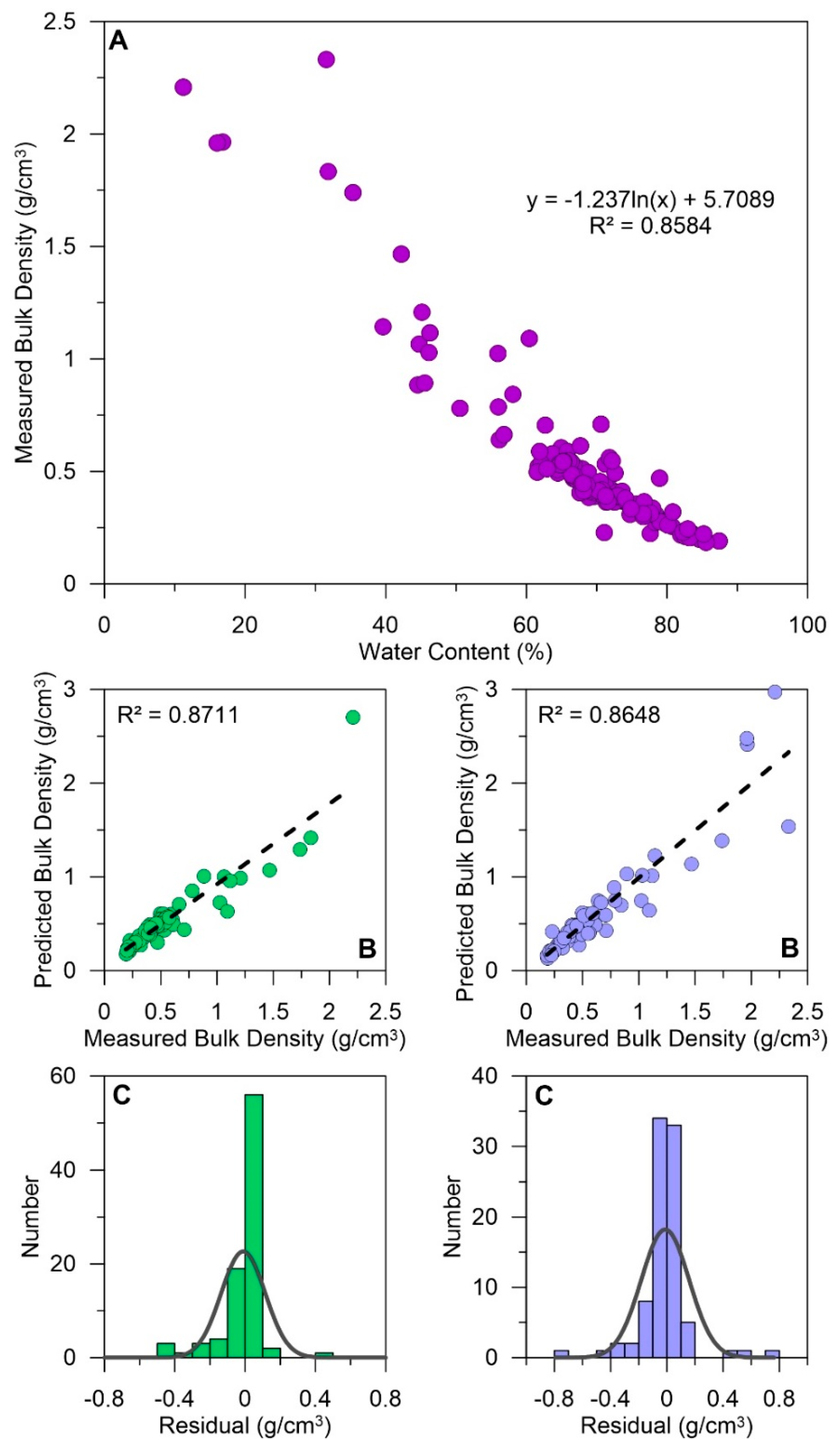
The relationship between water content and measured bulk density in the randomly selected lake core subsamples is best described by the logarithmic function y = −1.237ln(x) + 5.7089 with an r2 of 0.8584 (Figure 5A). When these data were split into two halves to test the efficacy of the logarithmic function in predicting bulk density, there was a linear relationship between the measured and predicted values in both trials with r2 ≥ 0.87. Residuals were generally smaller than 0.2 g/cm3 and followed a normal distribution (Figure 5B,C).
3.2. Phase II: Estimation of the Holocene Carbon Accumulation Rate and Carbon Stock
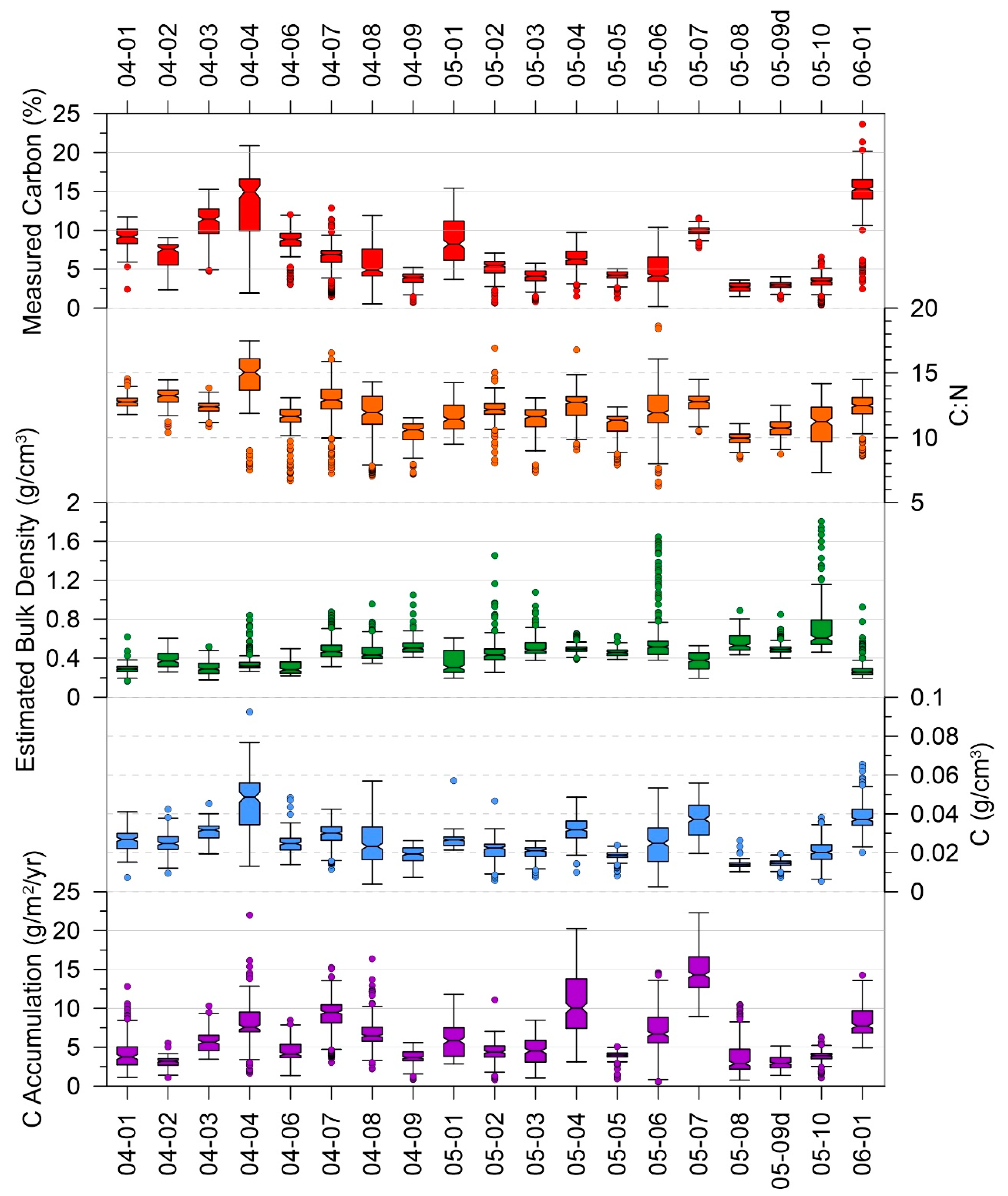
The relationship between water content and measured bulk density was used to predict bulk density for all of the Uinta lake sediment samples for which water content had previously been measured (Figure 6). The mean estimated bulk density is 0.52 g/cm3 (standard deviation of 0.32) and the median is 0.47 g/cm3. The 90th percentile range extends from 0.27 to 0.86 g/cm3. Previously measured values of percent carbon in the Holocene section of these cores range from 0.2% to 23.6% with a mean of 6.8% and a median of 5.9% (Figure 6). Multiplying these carbon abundances by the estimated bulk density values yielded the mass of carbon in each subsample. Summing these values for each core over the period 11,700 to 2000 BP and dividing by 9700 produced an estimate of long-term carbon accumulation rate. These rates range from 2.87 to 9.29 g/m2/yr. Multiplying these values by 11,700 generated an estimate of the carbon stock in each core ranging from 2.81 to 10.87 g/cm2 (Table 2).
3.3. Phase III: Extrapolating Using Spatial Predictors
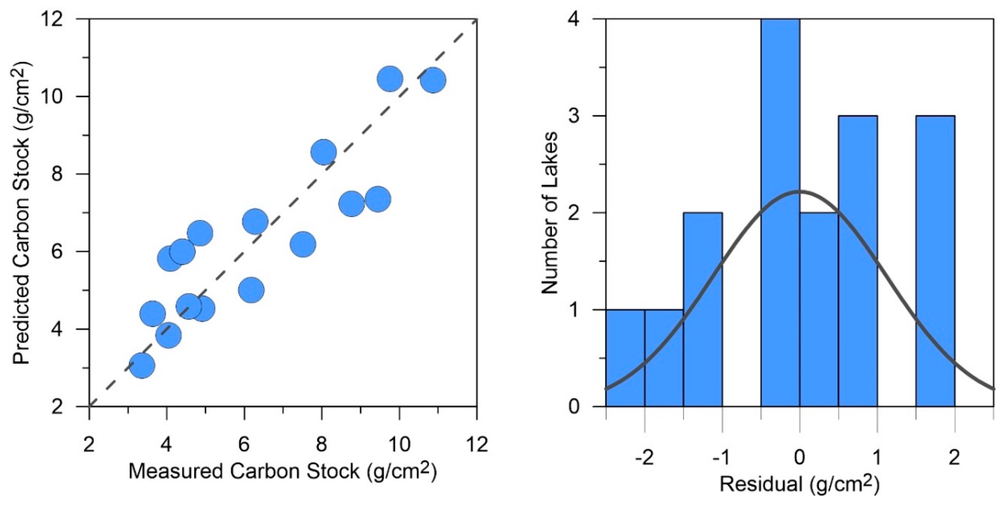
The result of the stepwise multilinear regression was an equation in which lake depth, lake area (log10) and lake complexity (log10) are predictors for Holocene carbon stock in the cored lakes. This regression had an information criterion of 15.289 and an adjusted r2 of 0.72 (Figure 7). All three variables were significant in the model, with P values <0.014 (Table 3). Residuals were generally symmetrically distributed within ±2 g/cm2 (Figure 7). Surprisingly, variables tabulated for the uphill buffer around in lake, such as mean slope or percent forest cover, did not exhibit a consistent relationship with carbon stock.
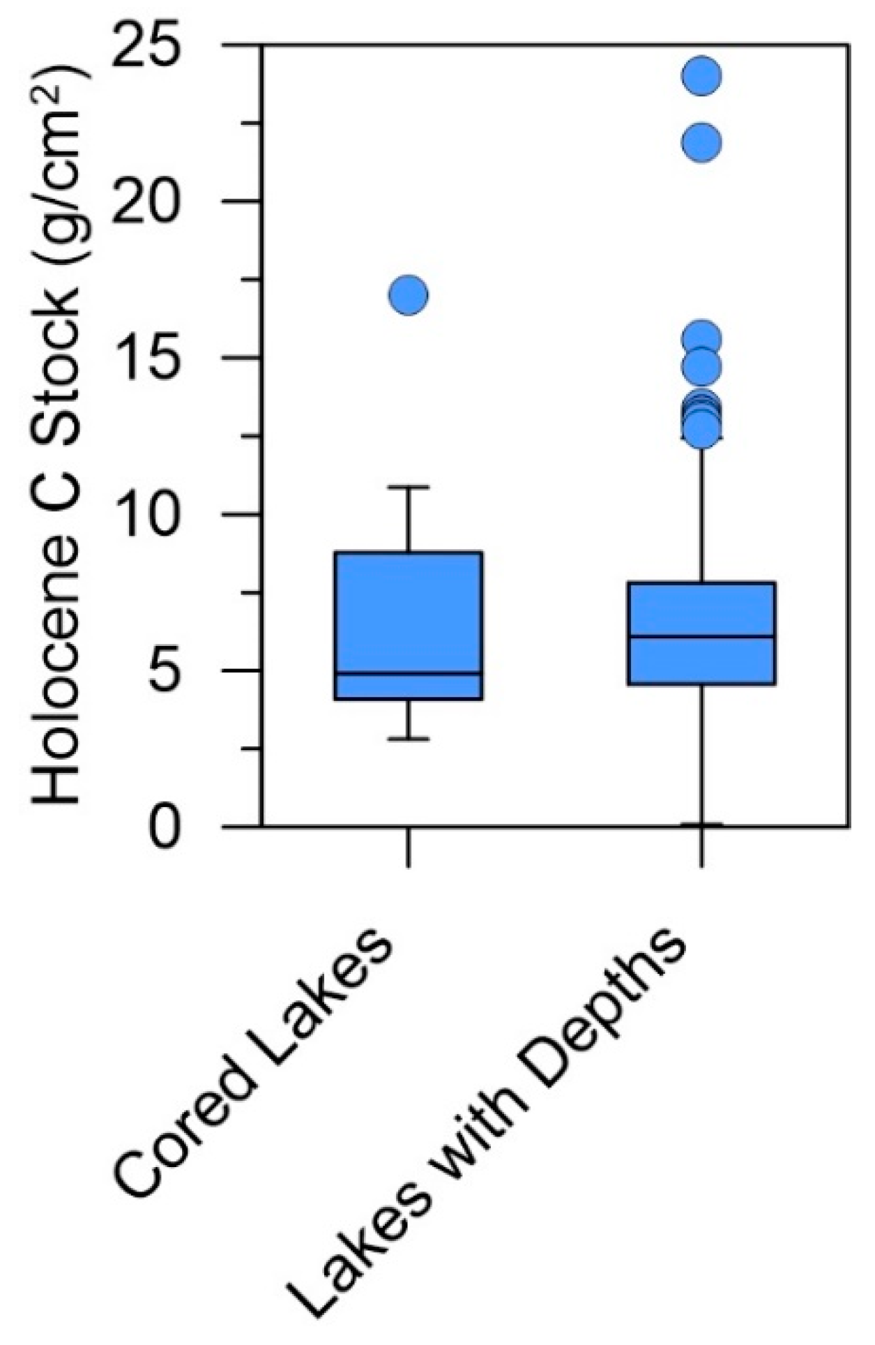
Results of the multilinear regression were then used to estimate carbon stock in the lakes for which depth data were available. Values range from to 0.09 to 24.0 g/cm2 with a mean of 6.36 g/cm2 (standard deviation 2.7) and a median of 6.09 g/cm2. The 90th percentile range extends from 3.6 to 9.6 g/cm2 (Figure 8). Dividing these stocks by 11,700 years yielded estimates of long-term carbon burial rates. Values range from to 0.1 to 20.5 g/m2/yr with a mean of 5.43 g/m2/yr (standard deviation 2.3) and a median of 5.21 g/m2/yr. The 90th percentile range extends from to 3.07 to 8.22 g/m2/yr.
3.4. Phase IV: Extrapolating to Landscape Scale
The final extrapolation to the landscape scale was accomplished using six different approximations of the “average” carbon stock in Uinta lakes (Table 4). After multiplying these values by the total area of lakes in the Uintas, and dividing by four as a conservative correction to accommodate changes in sediment thickness through each lake basin, it was concluded that these lakes accumulated between 5.9 × 10⁵ and 9.7 × 10⁵ metric tons of carbon over the past 11,700 years (Table 5). This corresponds to a long-term rate of between 50 and 83 metric tons of carbon per year (Table 5).
3.5. Carbon Content of Modern Sediment
The carbon content of recently deposited sediments in 7 Uinta lakes range from 3.2 to 19.2%. The highest values are found within 2 cm of the sediment-water interface.
4. Discussion
4.1. Carbon Accumulation Rates
Values of C:N provide information about the relative abundance of terrestrial and aquatic organic matter accumulating in a lake. Ratios <10 are typical of aquatic algae, whereas values >10 indicate increasing contributions of terrestrial material washing in from the surrounding watershed [45]. In two Uinta lakes, (04–09 and 05–08), all C:N values are <12, indicating that the organic matter is primarily algal (Figure 6). However, most of the studied lakes have average C:N values ~12 for the Holocene, with maximum values from 16 to 18 (Figure 6). This result indicates that a considerable amount of the organic matter accumulating in Uinta lakes is terrestrial in origin.
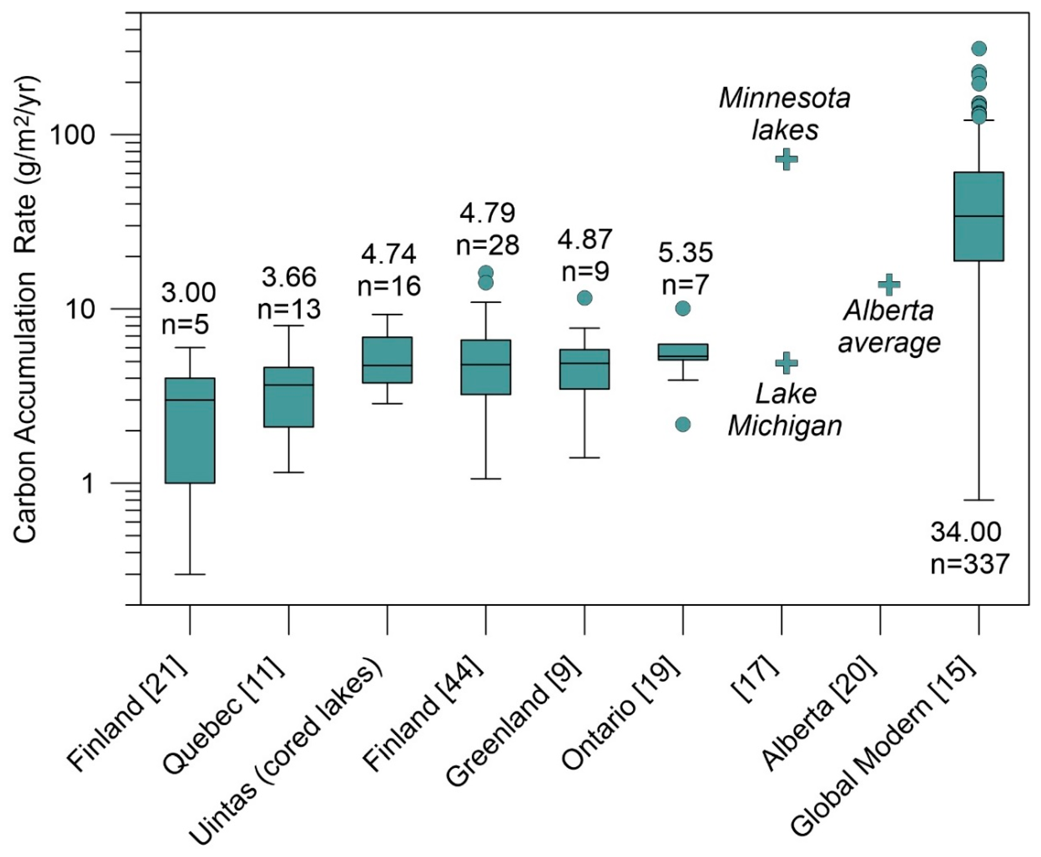
When lake size is plotted against carbon accumulation rate, it is clear that the Uinta lakes are generally smaller than those considered in many other studies (Figure 9A). However, the carbon accumulation rates determined for the Uinta lakes overlap strongly (Figure 10) with those reported for lakes at far more northerly latitudes, including in Ontario, northern Quebec, Finland, and Greenland [9,11,19,21,46]. In contrast, carbon accumulation rates in Uinta lakes are lower (Figure 10) than estimates for lakes in Alberta (15 g/m2/yr) [20] and dramatically lower than estimates for lakes in Minnesota (72 g/m2/yr) [17]. The median value for the cored Uinta lakes is most similar to values reported for lakes in Finland and southwestern Greenland ~25° (~2800 km) to the north. This median also matches the value estimated for Lake Michigan (5 g/m2/yr) [47], which is more than 128,000 times larger than the biggest lake cored in the Uintas. The trophic status of Uinta lakes (oligo- to mesotrophic) is not unusually low, and cannot be the sole explanation for this result. Rather, this result suggests that carbon accumulation rates in mid-latitude mountain lakes are more similar to those in boreal or arctic regions than in temperate regions that are geographically closer. Although it is perhaps logical that colder high-elevation lakes that endure long-periods of seasonal ice cover would be less productive than those in temperate lowland settings at similar latitudes, the magnitude of this difference is unexpectedly large. Future attempts to estimate lacustrine carbon storage at global scales should be careful to apply realistically low accumulation rates to mountain lakes even at lower latitudes if they are located at higher elevations.
The carbon accumulation rates for the lakes cored in the Uintas form a notably tight cluster in comparison with some of the other data reported in the literature (Figure 9A and Figure 10). This pattern likely reflects the relatively narrow range of lake dimensions targeted as part of the project for which these cores were originally collected. It is also apparent that some lakes in Greenland, Quebec, and Finland have carbon accumulation rates <2 g/m2/yr, which is the lower end of the values measured in the Uintas (Figure 9A). On the other hand, when the values estimated for all lakes in the Uintas for which depth data are available are plotted (Figure 9B), numerous lakes have values <2 g/m2/yr, indicating that the apparent minimum accumulation rate for Uinta lakes in Figure 9A is an artifact of the lakes that were originally cored.
4.2. The Carbon Content of Recent Sediments Relative to the Long-Term Average
The estimated carbon accumulation rates for Uinta lakes were calculated as an average for the interval 11,700 to 2000 BP, so caution is necessary when comparing them with modern rates. Nonetheless, it is notable how much lower the Uinta rates are (Figure 9B) than nearly all of the modern rates for lakes (excluding reservoirs) compiled in a recent global survey [15]. Indeed there is almost no overlap between the two populations when plotted vs. lake area (Figure 9B), and the greater median and much wider range for the modern data are clearly visible when compared with the long-term values determined from Holocene-length cores (Figure 10). This discrepancy may reflect the dominance of lakes in non-mountain settings in the modern compilation [15] as seen in Figure 1A. On the other hand, this difference is also consistent with recent studies, which have concluded that modern rates of carbon accumulation are higher than Holocene-scale averages, reflecting the effects of anthropogenic alterations to nutrient status and land cover [16,48].
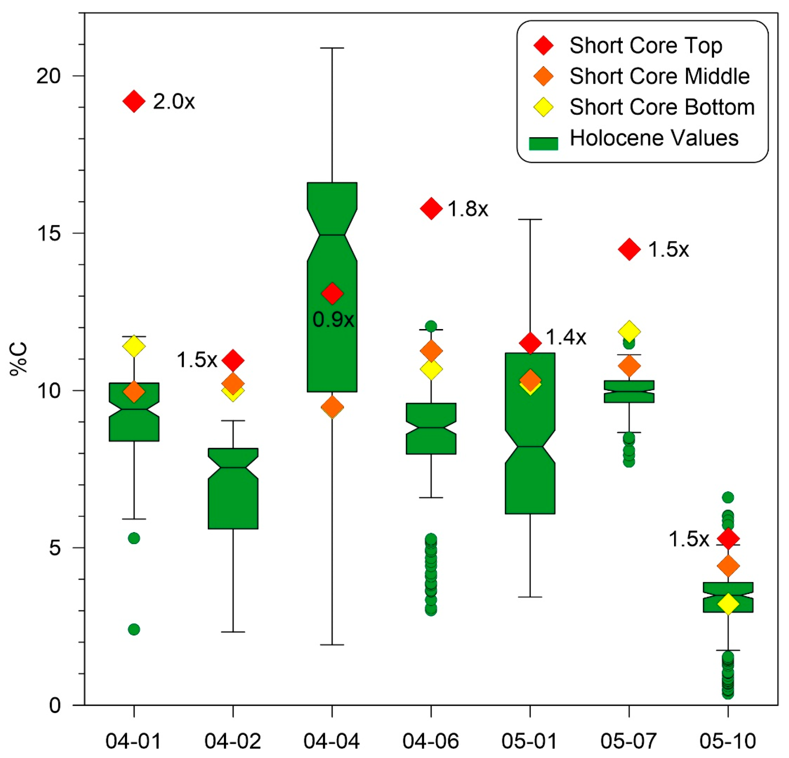
To clarify this uncertainty, it is useful to consider the %C values measured in young sediments collected from seven Uinta lakes with the gravity corer. Depth-age models are not available for these cores, so their %C values cannot be converted to accumulation rates. Nonetheless, it is illustrative to compare the carbon content in the near-surface sediments with the values measured between 11,700 and 2000 BP (Figure 11). In all but one lake, the carbon content of the uppermost 2 cm of sediment is from 1.4 to 2.0 times greater than the long-term median. The one lake in which this relationship does not hold (04–04), experienced a sustained stretch of uniquely high %C values in the early Holocene due to changes in the hydrology of its watershed [49]. In contrast, %C values measured for deeper sediment in each gravity core typically fall within the range of variability seen in the long-term records (Figure 11). Depth-age models based on 210Pb have been reported for two lakes in the Uintas, and in both of these, sediment below a depth of 9 cm was deposited before AD 1870 [50]. One of these lakes (Marshall Lake) was also considered in this study (04–01), and the dimensions, elevation, and setting of the other lake (Hidden Lake) are similar to the Uinta lakes from which long cores were collected. Thus, it is reasonable to conclude that the middle and bottom samples from the Uinta gravity cores were also deposited before the onset of any human perturbation of these remote water bodies. Correspondence of the %C values for the middle and bottom samples from the short cores with their corresponding long cores, and the elevated values in the top samples, therefore support the interpretation that carbon accumulation rates in Uinta lakes have increased in the Anthropocene. Previous work has presented diatom, sediment, and isotope evidence of enhanced productivity in Uinta lakes beginning in the mid-20th century and attributed this change to atmospheric deposition of nitrogen and phosphorus [31].
4.3. Carbon Pools
The total carbon pool of the Uintas is between 5.9 × 10⁵ and 9.7 × 10⁵ Mt (Table 5), depending on the value used to represent “average” Uinta lake sediment (Table 4). This total corresponds to a long-term rate of between 50 and 83 Mt of carbon per year. Even if the factor-of-4 reduction employed to correct for variations in sediment thickness within each lake basin is overly conservative, it is unlikely that lakes in the Uintas sequester more than a few hundred Mt of carbon annually.
Although this mountain range is notably lake-dense, with >6,000 lakes and >50 km2 of water surface area, total annual carbon sequestration in these lakes is very small compared to the amount of carbon humans emit annually through fossil fuel consumption. For example, as of 2009, Salt Lake City, the nearest metropolis to the Uintas, emitted 4.75 × 10⁶ Mt of CO2 per year, equivalent to 1.3 × 10⁶ Mt of carbon [51]. Therefore, each year, residents of Salt Lake City put a similar amount of carbon into the atmosphere as Uinta Mountain lakes have sequestered over the entire Holocene. Approximately one quarter of Salt Lake City carbon emissions (24%) is estimated to come from on-road vehicle traffic [51]. Thus, each year traffic in Salt Lake alone emits carbon equivalent to ~3000 years of lake sedimentation in the Uintas. Similarly, as of 2014, the average US citizen was responsible for the emission of 16.5 Mt of CO2 annually [52]. Therefore, at their Holocene rate, the >6000 lakes in the Uinta Mountains sequester as much carbon as ~20 or fewer average US residents, or ~10 Salt Lake city residents, who are responsible for more carbon emission than average (Salt Lake City Corporation, 2010). The carbon sink provided by Uinta Mountain lakes is therefore negligible compared to the amount of carbon emitted even locally by human activity, demonstrating the magnitude of perturbation to the global carbon cycle represented by anthropogenic emissions.
4.4. Limitations and Directions for Future Work
The design of this study represents an improvement on many previous projects in several ways. Foremost among these is that mountain lakes were directly investigated, rather than assuming that carbon accumulates in these environments at rates similar to those measured in lowland lakes. Inclusion of a large number of sediment cores, the analysis of these cores at 1 cm intervals, the use of a carbon analyzer for direct measurement of carbon content, and calculation of bulk density with a pycnometer for developing a transfer function with water content, are all steps that improve the resulting estimations. However, extrapolation from the cored lakes to the greater number of lakes for which less data are available required several assumptions that likely impacted the accuracy of the results. Most critically, due to the lack of detailed bathymetric and subsurface data, a conservative correction was applied to convert the carbon stocks measured in single depocenter cores to lake-wide carbon pool estimates. Although it was not an option in this study, previous work has demonstrated that a superior approach is to use a sub-bottom profiler to create a map of the sedimentary package underlying the lake bottom [7,11]. Additionally, since depth data could only be connected to 414 of the lakes, it was not possible to apply the relatively robust multilinear regression based on water depth, lake area, and shoreline complexity to all water bodies in the Uintas. Instead, six different estimates of “average” carbon stock were extrapolated to the range-wide lake dataset, with an obvious decrease in precision. Better estimates of the overall carbon pool would be possible if depth data were collected for additional lakes. Finally, it is intuitive that the hydrogeomorphic setting of each lake will control the amount of type of sediment that accumulates within it, including the amount of carbon. Previous work has demonstrated connections between lake setting in the Uintas and the amount of organic matter revealed by loss-on-ignition [12] measurements [53,54], so it was surprising that the watershed properties included as predictors in the multilinear regression failed to exert a significant control on the resulting carbon accumulation rate. On the other hand, perhaps the 100 m-wide lakeside buffer employed here failed to capture all salient aspects of each lake’s hydrogeomorphic setting. Future work could investigate this further, perhaps with more effective automated tools for delineating watershed boundaries.
5. Conclusions
This study employed a series of steps to extrapolate from 19 lake sediment cores to a range-wide estimate of the Holocene carbon storage in over 6000 lakes in the Uinta Mountains, Utah. Mountain lakes have been almost entirely overlooked in previous studies focused on lacustrine carbon inventories. Results indicate that Uinta Mountain lakes accumulated carbon over the Holocene at rates most similar to lakes in locations much farther north, such as Finland and Greenland. At the same time, accumulation rates in Uinta lakes are much lower than values reported for lakes relatively close by in Alberta and Minnesota. This result reveals that latitude alone is insufficient as a predictor for lacustrine carbon storage and underscores the danger inherent in broadly applying average accumulation rates to lakes in different biomes.
Although modern carbon accumulation rates could not be calculated, the carbon content of modern sediments in Uinta lakes are elevated up to two times above long-term rates for the Holocene. This pattern corroborates recent studies that have reported enhanced carbon accumulation rates in the Anthropocene. Given the almost complete lack of development around the Uinta lakes, most of which are located within a protected wilderness area, this recent enhancement of carbon accumulation is best explained by changes in nutrient status related to atmospheric deposition of nitrogen and phosphorus [31].
Finally, the total carbon pool in Uinta Mountain lakes is conservatively estimated as <10 × 105 Mt. Remarkably, this total is equivalent to the total carbon emitted by Salt Lake City, the nearest major urban area, in ~1 year. Annual carbon sequestration in Uinta lakes, based on long-term Holocene rates, is equivalent to the annual emissions of <20 average Americans. This result starkly underscores the magnitude of human perturbations to the global carbon cycle.
Supplementary Materials
The following are available online at https://0-www-mdpi-com.brum.beds.ac.uk/2571-550X/2/1/13/s1, Table S1: Carbon Content of Cored Lakes; Table S2: Carbon Content of Lakes with Depths; Table S3: All Lakes Carbon Estimates.
Author Contributions
Conceptualization, J.M.; methodology, J.M. and Q.B.; validation, J.M.; formal analysis, J.M. and Q.B.; investigation, J.M.; resources, J.M.; data curation, J.M.; writing—original draft preparation, J.M. and Q.B.; writing—review and editing, J.M.; visualization, J.M.; supervision, J.M.; project administration, J.M.; funding acquisition, J.M.
Funding
This research was funded by NSF-EAR-0345112, NSF-ATM-0402328, and EAR-0922940.
Acknowledgments
Cores used in this study were collected with the help of M. Devito, B. Laabs, D. Munroe, N. Oprandy, C. Plunkett, and numerous students. Thanks to D. Koerner with the Ashley National Forest for arranging critical logistical support. The comments of two anonymous reviewers were helpful in improving the manuscript.
Conflicts of Interest
The authors declare no conflict of interest.
References
- Verpoorter, C.; Kutser, T.; Seekell, D.A.; Tranvik, L.J. A global inventory of lakes based on high-resolution satellite imagery. Geophys. Res. Lett. 2014, 41, 6396–6402. [Google Scholar] [CrossRef]
- Cole, J.J.; Prairie, Y.T.; Caraco, N.F.; McDowell, W.H.; Tranvik, L.J.; Striegl, R.G.; Duarte, C.M.; Kortelainen, P.; Downing, J.A.; Middelburg, J.J.; et al. Plumbing the Global Carbon Cycle: Integrating Inland Waters into the Terrestrial Carbon Budget. Ecosystems 2007, 10, 172–185. [Google Scholar] [CrossRef]
- Tranvik, L.J.; Downing, J.A.; Cotner, J.B.; Loiselle, S.A.; Striegl, R.G.; Ballatore, T.J.; Dillon, P.; Finlay, K.; Fortino, K.; Knoll, L.B. Lakes and reservoirs as regulators of carbon cycling and climate. Limnol. Oceanogr. 2009, 54, 2298–2314. [Google Scholar] [CrossRef]
- Downing, J.A. Emerging global role of small lakes and ponds: Little things mean a lot. Limnética 2010, 29, 9–24. [Google Scholar]
- Mulholland, P.J.; Elwood, J.W. The role of lake and reservoir sediments as sinks in the perturbed global carbon cycle. Tellus 1982, 34, 490–499. [Google Scholar] [CrossRef]
- Einsele, G.; Yan, J.; Hinderer, M. Atmospheric carbon burial in modern lake basins and its significance for the global carbon budget. Glob. Planet. Chang. 2001, 30, 167–195. [Google Scholar] [CrossRef]
- Chmiel, H.E.; Kokic, J.; Denfeld, B.A.; Einarsdóttir, K.; Wallin, M.B.; Koehler, B.; Isidorova, A.; Bastviken, D.; Ferland, M.-È.; Sobek, S. The role of sediments in the carbon budget of a small boreal lake. Limnol. Oceanogr. 2016, 61, 1814–1825. [Google Scholar] [CrossRef]
- Kortelainen, P.; Pajunen, H.; Rantakari, M.; Saarnisto, M. A large carbon pool and small sink in boreal Holocene lake sediments. Glob. Chang. Biol. 2004, 10, 1648–1653. [Google Scholar] [CrossRef]
- Anderson, N.J.; D’andrea, W.; Fritz, S.C. Holocene carbon burial by lakes in SW Greenland. Glob. Chang. Biol. 2009, 15, 2590–2598. [Google Scholar] [CrossRef]
- Kastowski, M.; Hinderer, M.; Vecsei, A. Long-term carbon burial in European lakes: Analysis and estimate. Glob. Biogeochem. Cycles 2011, 25, GB3019. [Google Scholar] [CrossRef]
- Ferland, M.-E.; Giorgio, P.A.; Teodoru, C.R.; Prairie, Y.T. Long-term C accumulation and total C stocks in boreal lakes in northern Québec. Glob. Biogeochem. Cycles 2012, 26, GB0E04. [Google Scholar] [CrossRef]
- Dean, W.E., Jr. Determination of carbonate and organic matter in calcareous sediments and sedimentary rocks by loss on ignition; comparison with other methods. J. Sediment. Petrol. 1974, 44, 242–248. [Google Scholar]
- Dong, X.; Anderson, N.J.; Yang, X.; Shen, J. Carbon burial by shallow lakes on the Yangtze floodplain and its relevance to regional carbon sequestration. Glob. Chang. Biol. 2012, 18, 2205–2217. [Google Scholar] [CrossRef]
- Clow, D.W.; Stackpoole, S.M.; Verdin, K.L.; Butman, D.E.; Zhu, Z.; Krabbenhoft, D.P.; Striegl, R.G. Organic carbon burial in lakes and reservoirs of the conterminous United States. Environm. Sci. Technol. 2015, 49, 7614–7622. [Google Scholar] [CrossRef]
- Mendonça, R.; Müller, R.A.; Clow, D.; Verpoorter, C.; Raymond, P.; Tranvik, L.J.; Sobek, S. Organic carbon burial in global lakes and reservoirs. Nat. Commun. 2017, 8, 1694. [Google Scholar] [CrossRef] [PubMed]
- Heathcote, A.J.; Anderson, N.J.; Prairie, Y.T.; Engstrom, D.R.; del Giorgio, P.A. Large increases in carbon burial in northern lakes during the Anthropocene. Nat. Commun. 2015, 6, 10016. [Google Scholar] [CrossRef] [PubMed]
- Dean, W.E.; Gorham, E. Magnitude and significance of carbon burial in lakes, reservoirs, and peatlands. Geology 1998, 26, 535–538. [Google Scholar] [CrossRef]
- Sarmiento, J.L.; Sundquist, E.T. Revised budget for the oceanic uptake of anthropogenic carbon dioxide. Nature 1992, 356, 589. [Google Scholar] [CrossRef]
- Dillon, P.J.; Molot, L.A. Dissolved organic and inorganic carbon mass balances in central Ontario lakes. Biogeochemistry 1997, 36, 29–42. [Google Scholar] [CrossRef]
- Campbell, I.D.; Campbell, C.; Vitt, D.H.; Kelker, D.; Laird, L.D.; Trew, D.; Kotak, B.; LeClair, D.; Bayley, S. A first estimate of organic carbon storage in Holocene lake sediments in Alberta, Canada. J. Paleolimnol. 2000, 24, 395–400. [Google Scholar] [CrossRef]
- Einola, E.; Rantakari, M.; Kankaala, P.; Kortelainen, P.; Ojala, A.; Pajunen, H.; Mäkelä, S.; Arvola, L. Carbon pools and fluxes in a chain of five boreal lakes: A dry and wet year comparison. J. Geophys. Res. Biogeosci. 2011, 116, G03009. [Google Scholar] [CrossRef]
- Menounos, B. The water content of lake sediments and its relationship to other physical parameters: An alpine case study. Holocene 1997, 7, 207–212. [Google Scholar] [CrossRef]
- Bradley, W.H. Geomorphology of the North Flank of the Uinta Mountains; US Government Printing Office: Washington, DC, USA, 1936.
- Sears, J.; Graff, P.; Holden, G. Tectonic evolution of lower Proterozoic rocks, Uinta Mountains, Utah and Colorado. Geol. Soc. Am. Bull. 1982, 93, 990–997. [Google Scholar] [CrossRef]
- Dehler, C.M.; Porter, S.M.; De Grey, L.D.; Sprinkel, D.A.; Brehm, A. The Neoproterozoic Uinta Mountain Group revisited; a synthesis of recent work on the Red Pine Shale and related undivided clastic strata, northeastern Utah, U. S. A. Soc. Sediment. Geol. 2007, 86, 151–166. [Google Scholar]
- Munroe, J.S.; Laabs, B.J.C. Glacial Geologic Map of the Uinta Mountains Area, Utah and Wyoming; Utah Geological Survey: Cedar City, Utah, 2009.
- Munroe, J.; Laabs, B.; Shakun, J.; Singer, B.; Mickelson, D.; Refsnider, K.; Caffee, M. Latest Pleistocene advance of alpine glaciers in the southwestern Uinta Mountains, Utah, USA: Evidence for the influence of local moisture sources. Geology 2006, 34, 841–844. [Google Scholar] [CrossRef]
- Laabs, B.J.C.; Refsnider, K.A.; Munroe, J.S.; Mickelson, D.M.; Applegate, P.J.; Singer, B.S.; Caffee, M.W. Latest Pleistocene glacial chronology of the Uinta Mountains: Support for moisture-driven asynchrony of the last deglaciation. Quat. Sci. Rev. 2009, 28, 1171–1187. [Google Scholar] [CrossRef]
- Atwood, W.W. Lakes of the Uinta Mountains. Bull. Am. Geogr. Soc. 1908, 40, 12–17. [Google Scholar] [CrossRef]
- Atwood, W.W. Glaciation of the Uinta and Wasatch Mountains; US Government Printing Office: Washington, DC, USA, 1909; Volume 61.
- Hundey, E.J.; Moser, K.A.; Longstaffe, F.J.; Michelutti, N.; Hladyniuk, R. Recent changes in production in oligotrophic Uinta Mountain lakes, Utah, identified using paleolimnology. Limnol. Oceanogr. 2014, 59, 1987–2001. [Google Scholar] [CrossRef]
- Shaw, J.D.; Long, J.N. Forest ecology and biogeography of the Uinta Mountains, USA. Arct. Antarct. Alp. Res. 2007, 39, 614–628. [Google Scholar] [CrossRef]
- Munroe, J.S. Physical, chemical, and thermal properties of soils across a forest-meadow ecotone in the Uinta Mountains, Northeastern Utah, USA. Arct. Antarct. Alp. Res. 2012, 44, 95–106. [Google Scholar] [CrossRef]
- Munroe, J.S.; Mickelson, D.M. Last Glacial Maximum equilibrium-line altitudes and paleoclimate, northern Uinta Mountains, Utah, U.S.A. J.Glaciol. 2002, 48, 257–266. [Google Scholar] [CrossRef]
- Munroe, J.S. Holocene timberline and palaeoclimate of the northern Uinta Mountains, northeastern Utah, USA. Holocene 2003, 13, 175–185. [Google Scholar] [CrossRef]
- Munroe, J.S. Investigating the spatial distribution of summit flats in the Uinta Mountains of northeastern Utah, USA. Geomorphology 2006, 75, 437–449. [Google Scholar] [CrossRef]
- Munroe, J.S. Properties of alpine soils associated with well-developed sorted polygons in the Uinta Mountains, Utah, USA. Arct. Antarct. Alp. Res. 2007, 39, 578–591. [Google Scholar] [CrossRef]
- Bockheim, J.G.; Munroe, J.S. Organic carbon pools and genesis of alpine soils with permafrost: A review. Arct. Antarct. Alp. Res. 2014, 46, 987–1006. [Google Scholar] [CrossRef]
- Reasoner, M.A. Equipment and procedure improvements for a lightweight, inexpensive, percussion core sampling system. J. Paleolimnol. 1993, 8, 273–281. [Google Scholar] [CrossRef]
- Reimer, P.J.; Bard, E.; Bayliss, A.; Beck, J.W.; Blackwell, P.G.; Ramsey, C.B.; Buck, C.E.; Cheng, H.; Edwards, R.L.; Friedrich, M.; et al. IntCal13 and Marine13 radiocarbon age calibration curves 0–50,000 years cal BP. Radiocarbon 2013, 55, 1869–1887. [Google Scholar] [CrossRef]
- Blaauw, M. Methods and code for ‘classical’age-modelling of radiocarbon sequences. Quat. Geochronol. 2010, 5, 512–518. [Google Scholar] [CrossRef]
- Munroe, J.S.; Laabs, B.J. Combining radiocarbon and cosmogenic ages to constrain the timing of the last glacial-interglacial transition in the Uinta Mountains, Utah, USA. Geology 2017, 45, 171–174. [Google Scholar] [CrossRef]
- Munroe, J.S.; Klem, C.M.; Bigl, M.F. A lacustrine sedimentary record of Holocene periglacial activity from the Uinta Mountains, Utah, U.S.A. Quat. Res. 2013, 79, 101–109. [Google Scholar] [CrossRef]
- Blais, J.M.; Kalff, J. The influence of lake morphometry on sediment focusing. Limnol. Oceanogr. 1995, 40, 582–588. [Google Scholar] [CrossRef]
- Meyers, P.A.; Ishiwatari, R. Lacustrine organic geochemistry; an overview of indicators of organic matter sources and diagenesis in lake sediments. Org. Geochem. 1993, 20, 867–900. [Google Scholar] [CrossRef]
- Pajunen, H. Lake Sediments: Their Carbon Store and Related Accumulation Rates; Special Paper; Geological Survey Of Finland: Espoo, Finland, 2000; pp. 39–70.
- Rea, D.K.; Bourbonniere, R.A.; Meyers, P.A. Southern Lake Michigan sediments: Changes in accumulation rate, mineralogy, and organic content. J. Great Lakes Res. 1980, 6, 321–330. [Google Scholar] [CrossRef]
- Anderson, N.J.; Dietz, R.D.; Engstrom, D.R. Land-use change, not climate, controls organic carbon burial in lakes. Proc. R. Soc. B Biol. Sci. 2013, 280, 20131278. [Google Scholar] [CrossRef]
- Corbett, L.B.; Munroe, J.S. Investigating the influence of hydrogeomorphic setting on the response of lake sedimentation to climatic changes in the Uinta Mountains, Utah, USA. J. Paleolimnol. 2010, 44, 311–325. [Google Scholar] [CrossRef]
- Reynolds, R.L.; Mordecai, J.S.; Rosenbaum, J.G.; Ketterer, M.E.; Walsh, M.K.; Moser, K.A. Compositional changes in sediments of subalpine lakes, Uinta Mountains (Utah): Evidence for the effects of human activity on atmospheric dust inputs. J. Paleolimnol. 2010, 44, 161–175. [Google Scholar] [CrossRef]
- Salt Lake Community Corporation Salt Lake City Community Carbon Footprint. Available online: http://www.slcdocs.com/slcgreen/SLC%20Community%20Carbon%20Footprint%20Report%20(2).pdf (accessed on 19 February 2019).
- The World Bank CO2 Emissions (Metric Tons Per Capita). Available online: https://data.worldbank.org/indicator/EN.ATM.CO2E.PC (accessed on 19 February 2019).
- Munroe, J.S. Exploring relationships between watershed properties and Holocene loss-on-ignition records in high-elevation lakes, southern Uinta Mountains, Utah, U.S.A. Arct. Antarct. Alp. Res. 2007, 39, 556–565. [Google Scholar] [CrossRef]
- Munroe, J.S. Hydrogeomorphic controls on Holocene lacustrine loss-on-ignition records. J. Paleolimnol. 2019, 61, 53–68. [Google Scholar] [CrossRef]
Figure 1.
Location of the study area. (A) Global distribution of previous studies that calculated rates of carbon accumulation in lakes. Red squares represent Holocene-length studies, along with shading for Alberta, Canada [20] and various European countries where studies have been completed [10]. Blue dots represent locations where modern rates of carbon burial in lakes have been calculated, as summarized in recent work [15]. The yellow triangle marks the location of the Uinta Mountains in the western US. (B) Lakes of the Uinta Mountain range in Utah (denoted by the yellow triangle in Panel A) displayed over a digital elevation model with hillshading to accentuate topography. Areas covered by glaciers at the Last Glacial Maximum (LGM) are shown in green [26]. Cored lakes are marked with circles and the box delineates the inset. (C) Inset showing typical lake density in the Uinta Mountains displayed over a true-color aerial image with hillshading. Areas covered by glaciers during the LGM are shown in green.

Figure 2.
Schematic showing the four phases of extrapolation in this study and the methods employed at each step.
Figure 2.
Schematic showing the four phases of extrapolation in this study and the methods employed at each step.

Figure 3.
Distribution of randomly selected samples in sediment cores from 10 lakes, plotted against depth below the top of each core. Because cores were artificially truncated, core tops do not always correspond with the modern sediment-water interface. Colored lines in background denote the length of each core. Black arrows note 14C age control in each core. Radiocarbon ages and resulting depth-age models are presented in (Munroe, GSA Bulletin, in press).

Figure 4.
Distribution of elevations, areas, and depths for Uinta lakes.

Figure 5.
Water content and bulk density in Uinta lake sediments. (A) Relationship between water content and bulk density. (B) This dataset was randomly split in half (twice) and the two halves were used to test the robustness of the relationship. In both cases, moisture content proved to be a valid predictor of bulk density. (C) Residuals were <0.2 g/cm3 when predicted values were compared with measured values.

Figure 6.
Measured percent carbon, C:N ratio, estimated bulk density, calculated carbon content, and carbon accumulation rate in the Holocene section (11,700 BP to present) of 19 Uinta lake sediment cores.
Figure 6.
Measured percent carbon, C:N ratio, estimated bulk density, calculated carbon content, and carbon accumulation rate in the Holocene section (11,700 BP to present) of 19 Uinta lake sediment cores.

Figure 7.
Results of predicting carbon stock with the multilinear regression (Table 3).
Figure 7.
Results of predicting carbon stock with the multilinear regression (Table 3).

Figure 8.
Boxplot comparing Holocene carbon stock in the 19 cored lakes with the stock estimated in the 414 lakes for which depth data are available.
Figure 8.
Boxplot comparing Holocene carbon stock in the 19 cored lakes with the stock estimated in the 414 lakes for which depth data are available.

Figure 9.
Plots of lake area and carbon accumulation rate. (A) Log-log plot of lake area vs. carbon accumulation rate for studies based on Holocene-length records. Uinta lakes have rates more similar to those of lakes in locations much farther north. (B) Log-log plot (same axis dimensions) of carbon accumulation rates in Uinta lakes (measured and estimated) and modern sedimentation rates in a recent global compilation [15].

Figure 10.
Boxplot of reported carbon accumulation rates.

Figure 11.
Boxplot of carbon contents measured in Uinta lakes from Holocene-length long cores, and surface sediments collected with a gravity corer. Numbers indicate the enhancement of the modern value (red diamond) over the Holocene median.
Figure 11.
Boxplot of carbon contents measured in Uinta lakes from Holocene-length long cores, and surface sediments collected with a gravity corer. Numbers indicate the enhancement of the modern value (red diamond) over the Holocene median.


Table 1.
Locations and Dimensions of Cored Lakes.
| Lake ID | Lake Name | Latitude North DD MM.mmm | Longitude West DD MM.mmm | Elevation asl m | Water Depth m | Lake Area ha | AW/AL * | Hydrology ** | Core Length cm | Holocene Thickness cm | Water Measurements n | Carbon Measurements n |
|---|---|---|---|---|---|---|---|---|---|---|---|---|
| 4-01 | Marshall | 40° 40.538 | 110° 52.452 | 3043 | 10.7 | 8.0 | 7.5 | 1 | 190 | 150 | 190 | 184 |
| 04-02 | Hoover | 40° 40.824 | 110° 50.824 | 3018 | 7.9 | 7.8 | 17.8 | 4 | 156 | 127 | 156 | 155 |
| 04-03 | Pyramid | 40° 39.192 | 110° 54.094 | 2957 | 10.7 | 5.8 | 13.3 | 1 | 180 | 180 | 180 | 179 |
| 04-04 | Elbow | 40° 47.619 | 110° 02.502 | 3326 | 10.7 | 10.0 | 33.5 | 2 | 217 | 159 | 217 | 215 |
| 04-06 | Swasey | 40° 40.048 | 110° 28.000 | 3267 | 9.5 | 14.6 | 21.7 | 2 | 198 | 154 | 198 | 192 |
| 04-07 | Spider | 40° 42.019 | 110° 28.756 | 3316 | 12.8 | 8.1 | 44.8 | 3 | 324 | 324 | 324 | 324 |
| 04-08 | Little Superior | 40° 44.003 | 110° 28.461 | 3417 | 9.5 | 6.0 | 51.8 | 3 | 264 | 264 | 264 | 263 |
| 04-09 | North Star | 40° 45.195 | 110° 27.075 | 3474 | 5.8 | 5.8 | 49.7 | 4 | 198 | 183 | 198 | 198 |
| 05-01 | Reader | 40° 47.445 | 110° 03.583 | 3341 | 4.0 | 4.8 | 11.3 | 2 | 246 | 233 | 246 | 246 |
| 05-02 | Ostler | 40° 45.579 | 110° 46.749 | 3218 | 5.2 | 5.3 | 21.9 | 2 | 213 | 213 | 212 | 212 |
| 05-03 | Kermsuh | 40° 44.876 | 110° 49.926 | 3145 | 5.2 | 3.9 | 68.2 | 3 | 219 | 219 | 219 | 219 |
| 05-04 | Ryder | 40° 43.540 | 110° 49.688 | 3243 | 17.4 | 8.6 | 17.3 | 3 | 347 | 317 | 347 | 347 |
| 05-05 | Lower Red Castle | 40° 48.793 | 110° 27.762 | 3279 | 9.1 | 17.6 | 65.8 | 4 | 142 | 130 | 142 | 142 |
| 05-06 | Bald | 40° 52.030 | 110° 29.540 | 3367 | 7.0 | 2.2 | 14.5 | 1 | 355 | 341 | 355 | 355 |
| 05-07 | Hessie | 40° 52.102 | 110° 25.742 | 3237 | 6.1 | 5.3 | 7.5 | 1 | 258 | 258 | 258 | 258 |
| 05-08 | Deadhorse | 40° 44.711 | 110° 40.381 | 3316 | 12.5 | 5.8 | 12.8 | 3 | 199 | 205 | 199 | 194 |
| 05-09d | Island | 40° 49.796 | 110° 08.684 | 3285 | 11.4 | 45.3 | 24.1 | 4 | 308 | 213 | 308 | 308 |
| 05-10 | Taylor | 40° 47.193 | 110° 05.478 | 3421 | 11.0 | 9.0 | 35.4 | 3 | 270 | 219 | 257 | 257 |
| 06-01 | Upper Lily Pad | 40° 37.665 | 110° 15.993 | 3129 | 9.8 | 4.0 | 76.3 | 2 | 371 | 245 | 371 | 371 |
* Ratio of watershed area to lake area. ** 1—no inlet or outlet; 2—little or no obvious inflow, weak outflow; 3—modest inflow and outflow; 4—robust inflow and outflow.
Table 2.
Calculated and Predicted Holocene C.
| Lake ID | Lake Name | Holocene C g/cm2 | Predicted C g/cm2 | Accumulation Rate g/m2/yr |
|---|---|---|---|---|
| 04-01 | Marshall Lake | 4.09 | 5.82 | 3.49 |
| 04-02 | Hoover Lake | 3.63 | 4.4 | 3.10 |
| 04-03 | Pyramid Lake | 6.27 | 6.77 | 5.36 |
| 04-04 | Elbow Lake | 8.77 | 7.23 | 7.49 |
| 04-06 | Swasey Lake | 4.57 | 4.58 | 3.91 |
| 04-07 | Spider Lake | 9.76 | 10.45 | 8.34 |
| 04-08 | Little Superior Lake | 7.51 | 6.19 | 6.42 |
| 04-09 | North Star Lake | 4.04 | 3.84 | 3.45 |
| 05-01 | Reader Lake | 6.18 | 5.01 | 5.28 |
| 05-02 | Ostler Lake | 4.91 | 4.53 | 4.20 |
| 05-03 | Kermsuh Lake | 4.86 | 6.47 | 4.15 |
| 05-04 | Ryder Lake | 10.87 | 10.42 | 9.29 |
| 05-05 | Lower Red Castle Lake | 4.51 | 4.17 | -- |
| 05-06 | Bald Lake | 8.05 | 8.56 | 6.88 |
| 05-07 | Hessie Lake | 17.02 | 4.74 | -- |
| 05-08 | Dead Horse Lake | 2.81 | 8.74 | -- |
| 05-09d | Island Lake | 3.35 | 3.06 | 2.87 |
| 05-10 | Taylor Lake | 4.40 | 6 | 3.76 |
| 06-01 | Upper Lily Pad | 9.44 | 7.35 | 8.07 |
Table 3.
Multilinear Regression Summary.
| Model Term | Coefficient | Significance |
|---|---|---|
| Intercept | 34.379 | 0.000 |
| Lake Area (log10) | −7.193 | 0.000 |
| Lake Depth | 0.559 | 0.000 |
| Shoreline Complexity (log10) | 11.154 | 0.014 |
Table 4.
Average Carbon Stocks and Accumulation Rates in Uinta Lakes.
| Cored Lakes n = 19 | Carbon Stock g/cm2 | Accumulation Rate g/m2/yr | Lakes with Depths n = 414 | Carbon Stock g/cm2 | Accumulation Rate g/m2/yr |
|---|---|---|---|---|---|
| max | 17.02 | 14.55 | max | 23.99 | 20.51 |
| min | 2.81 | 2.40 | min | 0.09 | 0.08 |
| median | 4.91 | 4.20 | median | 6.09 | 5.21 |
| mean | 6.58 | 5.63 | mean | 6.35 | 5.43 |
Table 5.
Estimates of the Total Carbon Pool in Uinta Lakes.
| Cored Lakes n = 19 | Total Carbon Pool Mt | Accumulation Rate Mt/yr | Lakes with Depths n = 414 | Total Carbon Pool Mt | Accumulation Rate Mt/yr |
|---|---|---|---|---|---|
| median | 587622 | 50 | median | 729111 | 62 |
| mean | 787766 | 67 | mean | 760713 | 65 |
| smallest 25% | 800454 | 68 | smallest 25% | 967201 | 83 |
© 2019 by the authors. Licensee MDPI, Basel, Switzerland. This article is an open access article distributed under the terms and conditions of the Creative Commons Attribution (CC BY) license (http://creativecommons.org/licenses/by/4.0/).
Share and Cite
MDPI and ACS Style
Munroe, J.; Brencher, Q. Holocene Carbon Burial in Lakes of the Uinta Mountains, Utah, USA. Quaternary 2019, 2, 13. https://0-doi-org.brum.beds.ac.uk/10.3390/quat2010013
AMA Style
Munroe J, Brencher Q. Holocene Carbon Burial in Lakes of the Uinta Mountains, Utah, USA. Quaternary. 2019; 2(1):13. https://0-doi-org.brum.beds.ac.uk/10.3390/quat2010013
Chicago/Turabian StyleMunroe, Jeffrey, and Quinn Brencher. 2019. "Holocene Carbon Burial in Lakes of the Uinta Mountains, Utah, USA" Quaternary 2, no. 1: 13. https://0-doi-org.brum.beds.ac.uk/10.3390/quat2010013