Metamodels Resulting from Two Different Geometry Morphing Approaches Are Suitable to Direct the Modification of Structure-Born Noise Transfer in the Digital Design Phase


Abstract
:
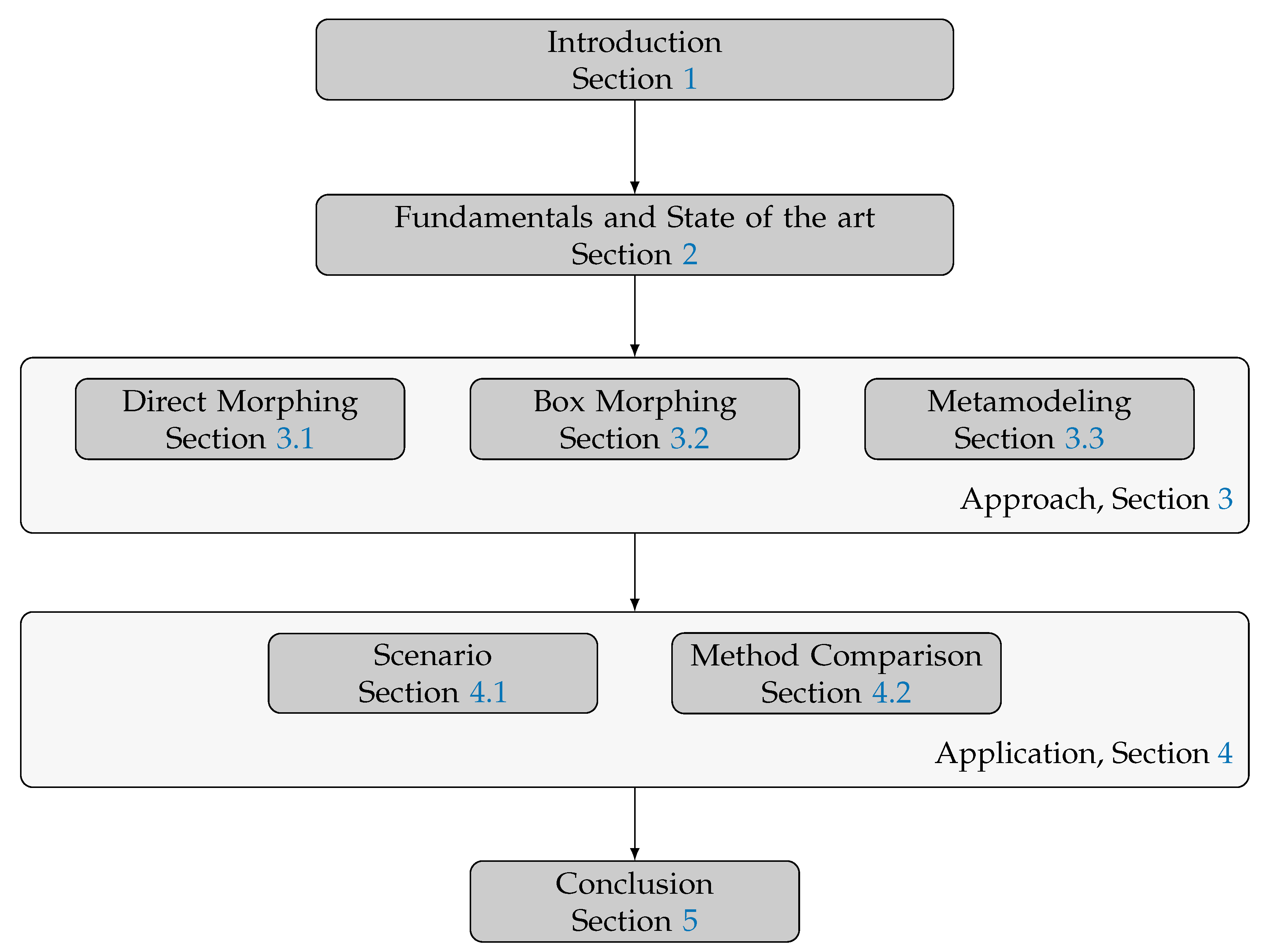
1. Introduction
2. Fundamentals and State of the Art
2.1. NVH Optimization in the Digital Design Phase
2.2. Morphing
Application of Morphing
2.3. Morphing Alternatives
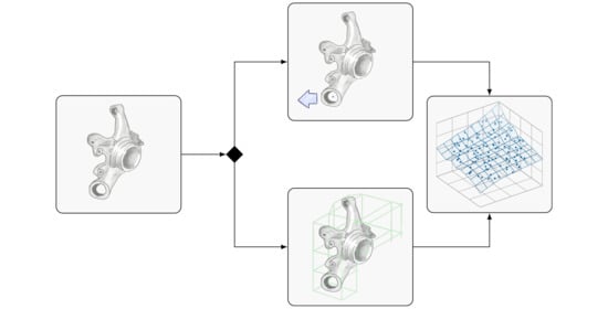
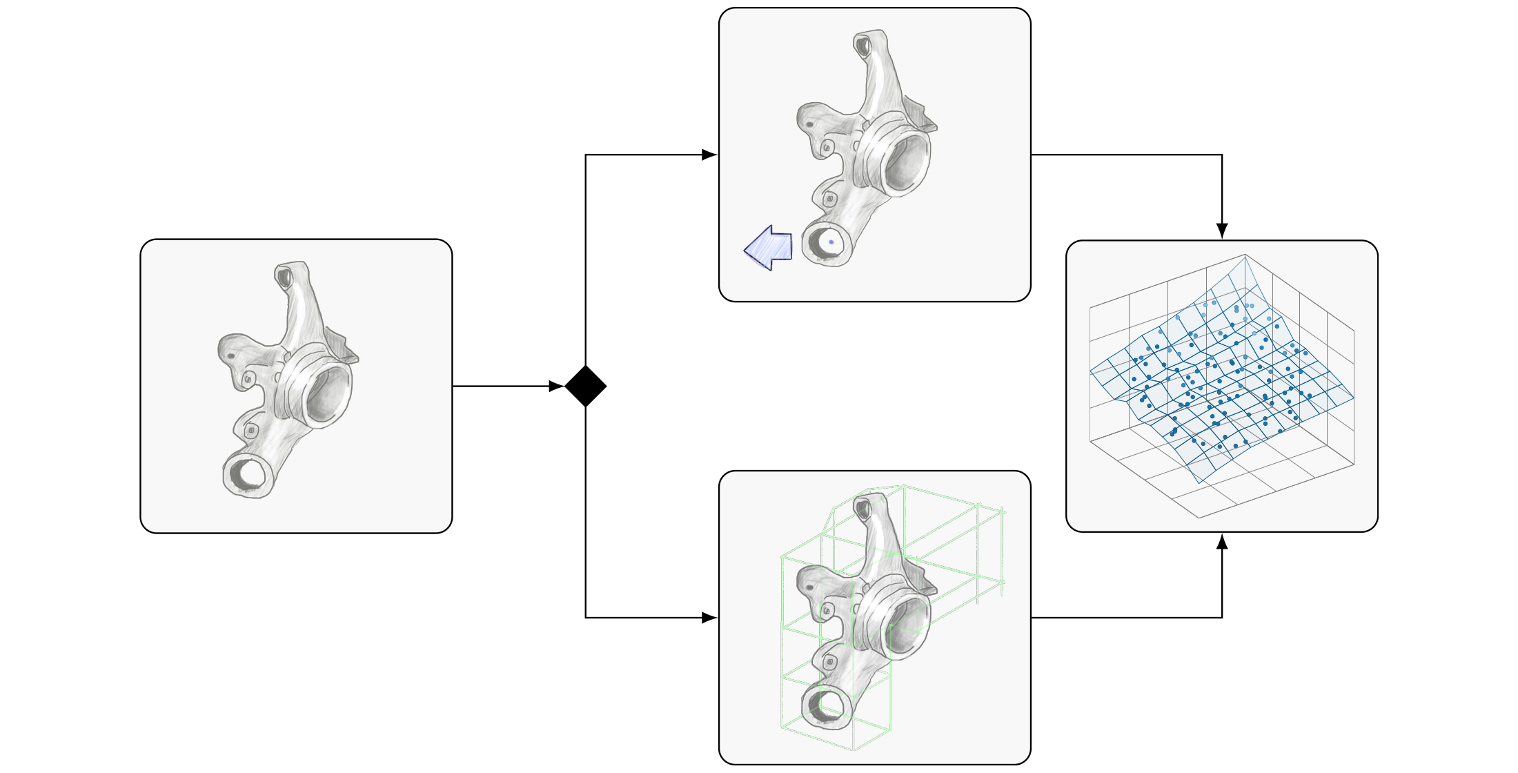
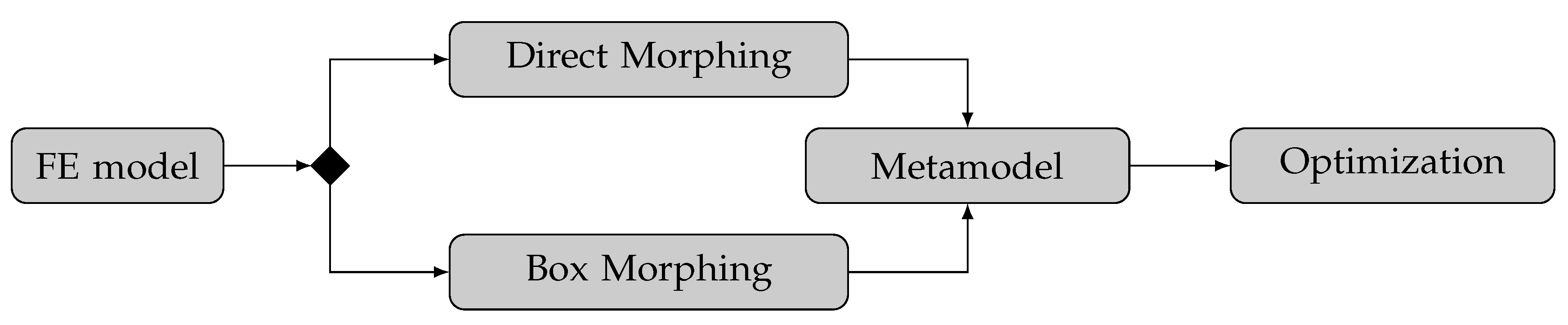
3. Method
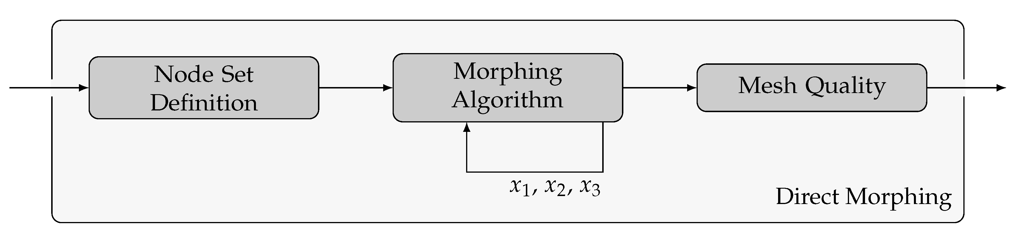
3.1. Direct Morphing Approach
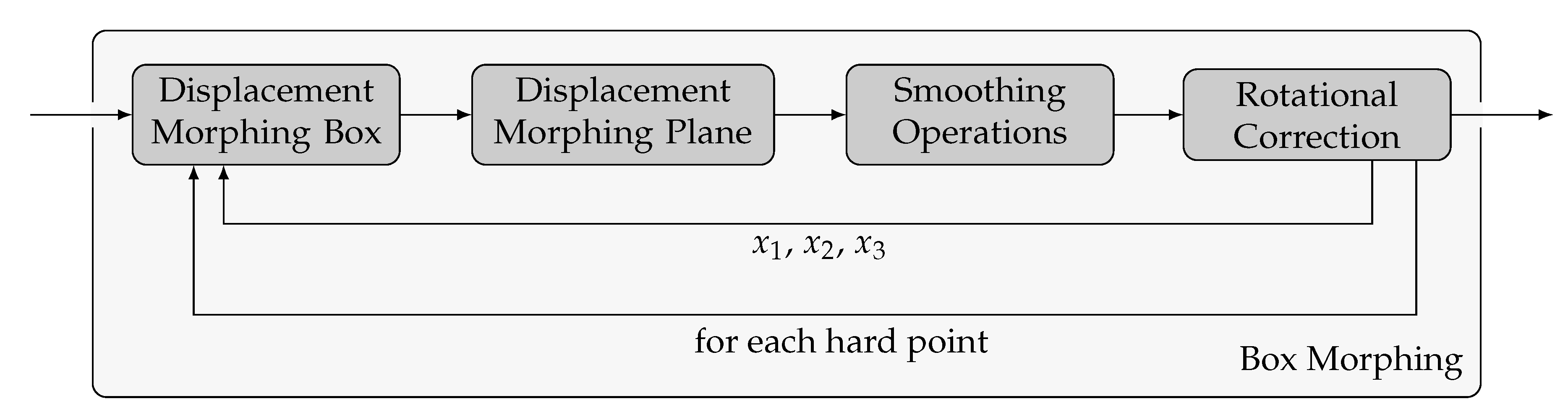
3.2. Box Morphing Approach
3.3. Metamodeling
4. Application
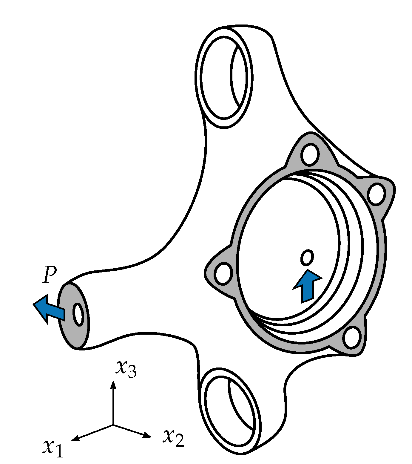
4.1. Scenario
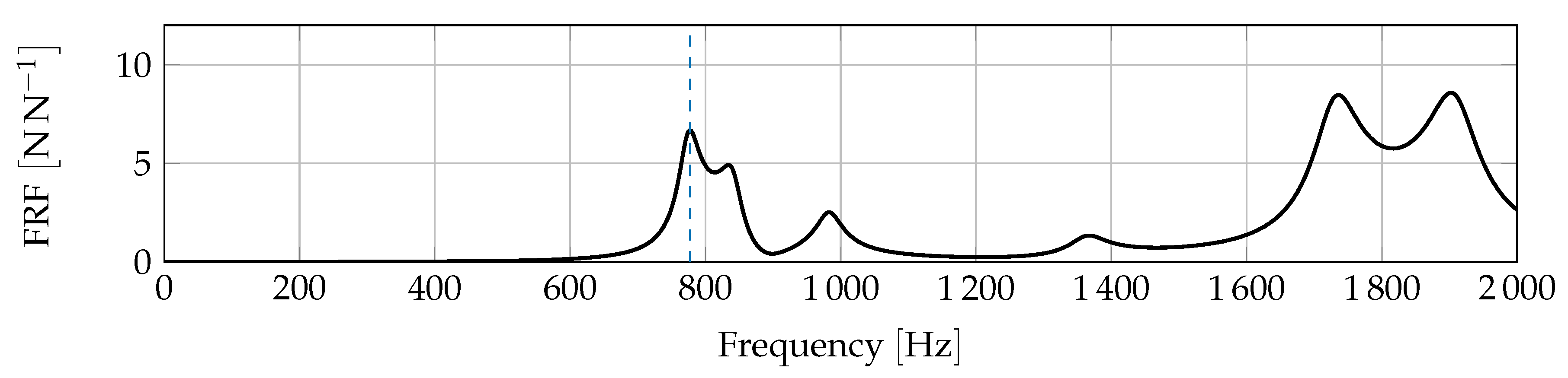
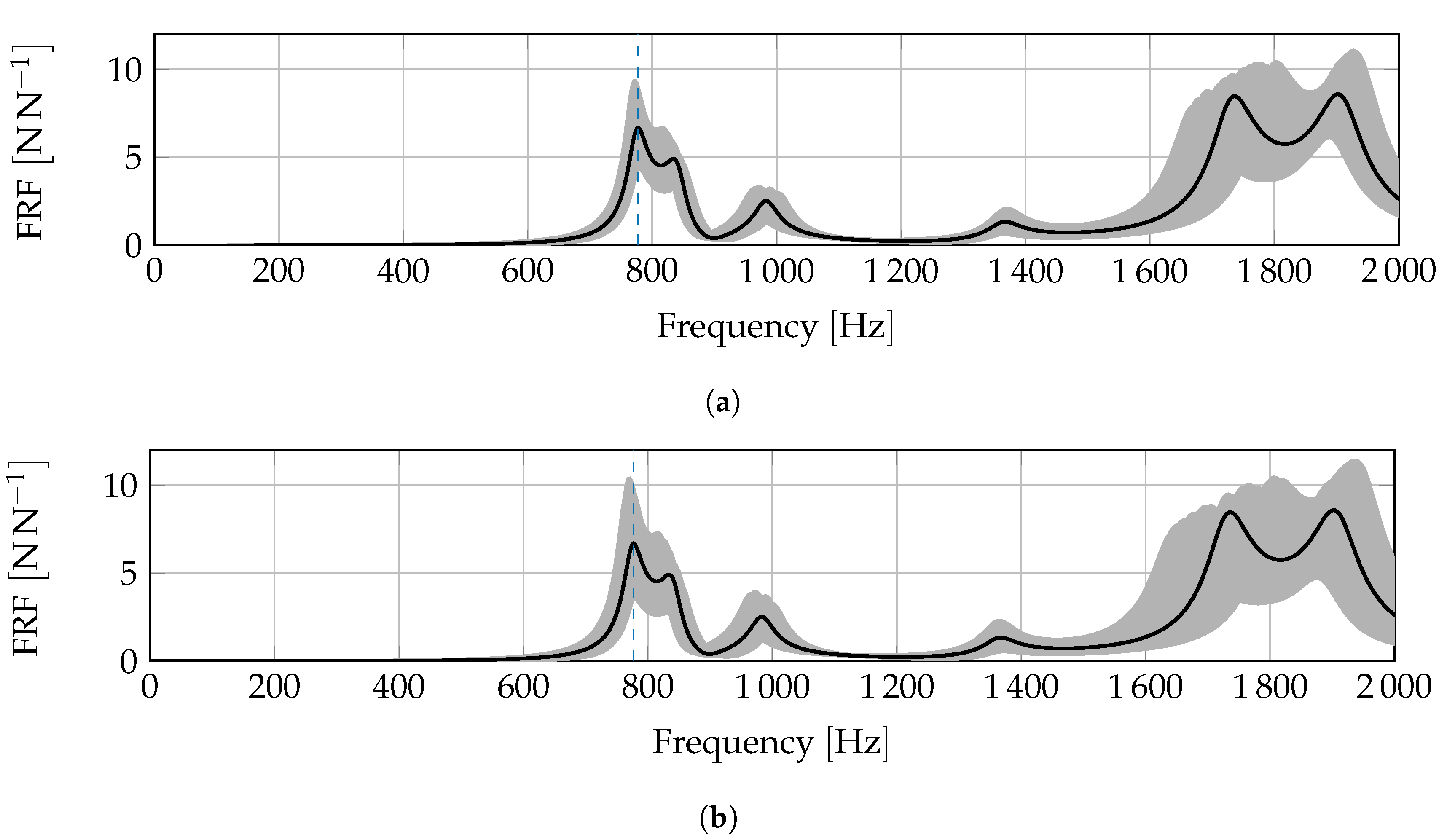
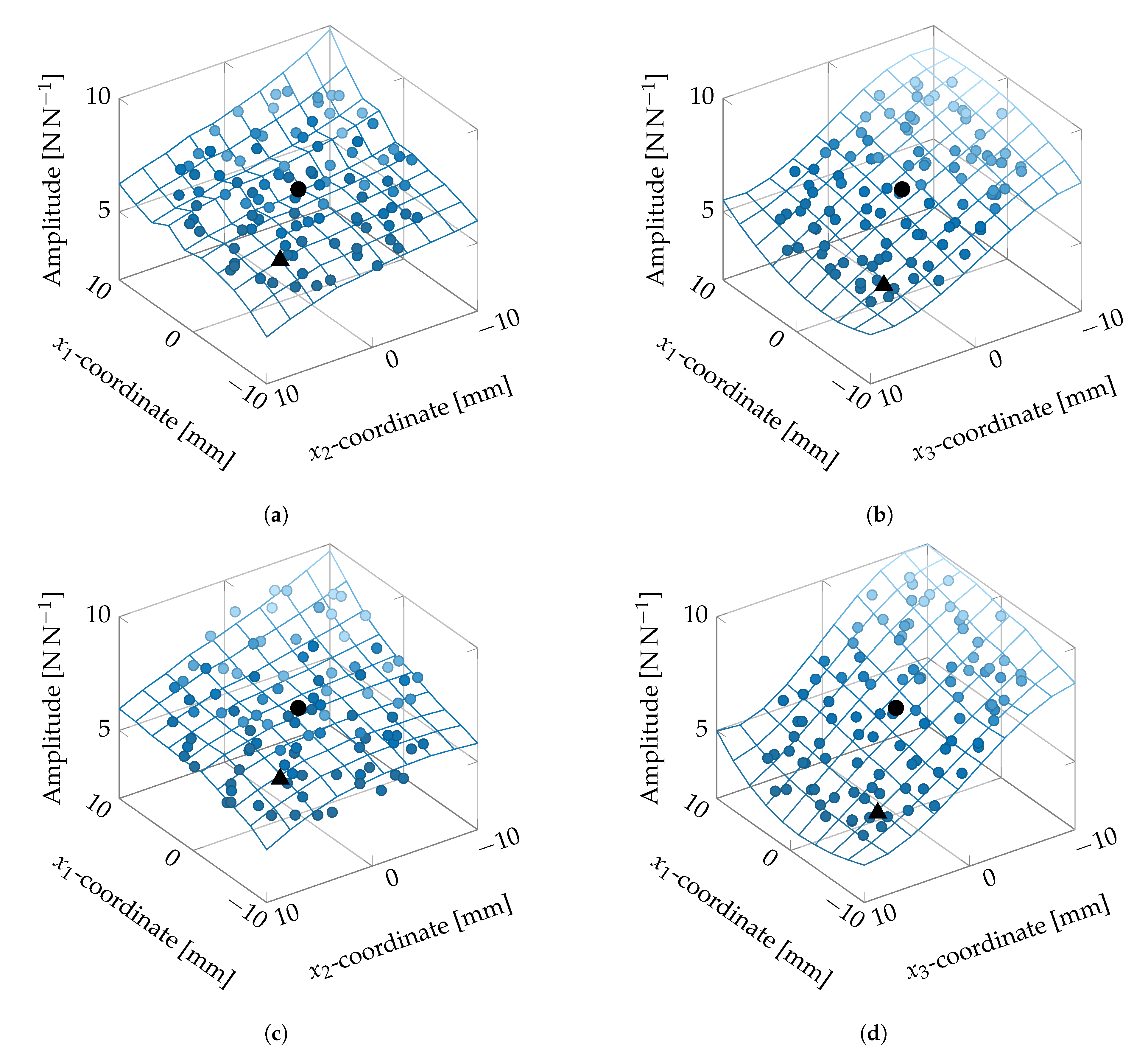
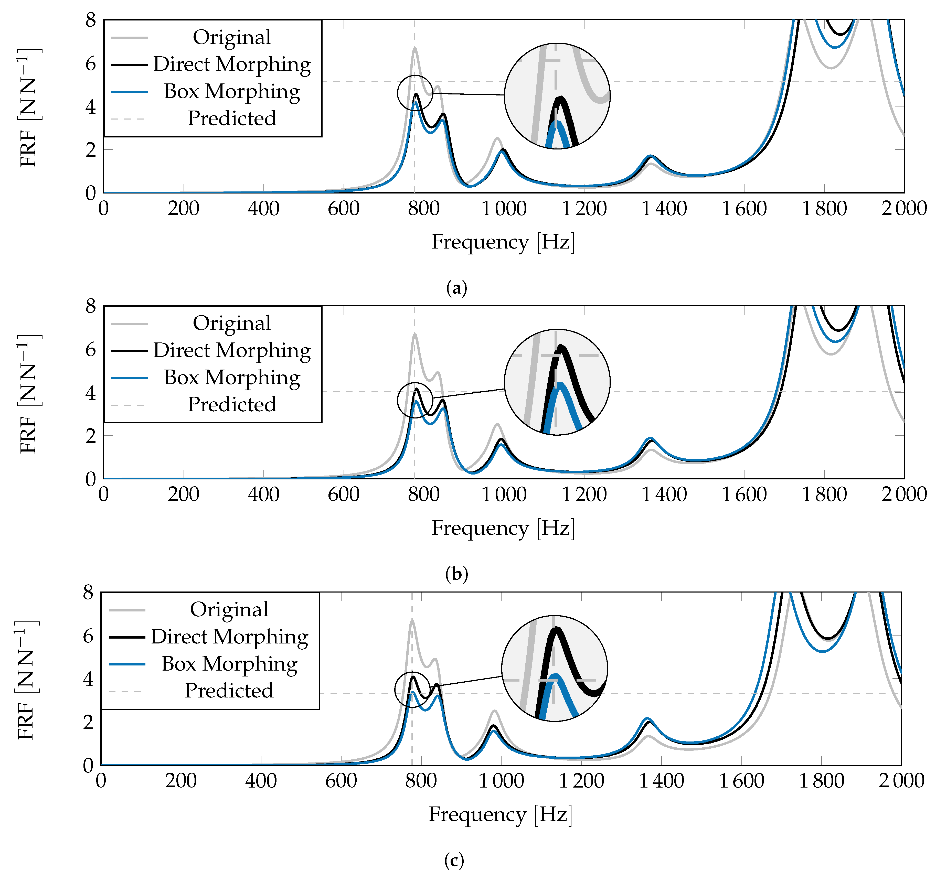
4.2. Method Comparison
5. Conclusions
Author Contributions
Funding
Acknowledgments
Conflicts of Interest
Abbreviations
| CAD | Computer Aided Design |
| CAE | Computer Aided Engineering |
| EFFD | Extended-Free-Form-Deformation |
| FE | Finite Element |
| FEM | Finite Element Method |
| FFD | Free-Form-Deformation |
| FRF | Frequency Response Function |
| NVH | Noise, Vibration and Harshness |
References
- Mantovani, M. Rolling noise does not evoke an emotional response. ATZ Worldw. 2018, 120, 18–21. [Google Scholar] [CrossRef]
- Rambacher, C.; Ehrt, T.; Sell, H. Vibration optimisation of entire axles. ATZ Worldw. 2017, 119, 50–55. [Google Scholar] [CrossRef]
- van der Auweraer, H.; van Langenhove, T.; Brughmans, M.; Bosmans, I.; Masri, N.; Donders, S. Application of mesh morphing technology in the concept phase of vehicle development. Int. J. Veh. Des. 2007, 43, 281–305. [Google Scholar] [CrossRef]
- Helm, D.; Huf, A.; Zimmer, H.; Kondziella, R. Anforderungen in der frühen Phase der Gesamtfahrzeugauslegung. VDI-Berichte 2012, 2169, 21–40. [Google Scholar]
- TrelleborgVibracoustic. Schwingungstechnik im Automobil: Grundlagen, Werkstoffe, Konstruktion, Berechnung und Anwendungen, 1st ed.; Vogel Business Media: Würzburg, Germany, 2015. [Google Scholar]
- De Gaetano, G.; Mundo, D.; Vena, G.; Kroiss, M.; Cremers, L. A study on vehicle body concept modelling: Beam to joint connection and size optimization of beam-like structures. In Proceedings of the ISMA 2014 Including USD 2014, Leuven, Belgium, 15–17 September 2014; pp. 1653–1664. [Google Scholar]
- Stigliano, G.; Mundo, D.; Donders, S.; Tamarozzi, T. Advanced Vehicle Body Concept Modeling Approach Using Reduced Models of Beams and Joints. In Proceedings of the ISMA 2010 Including USD 2012, Leuven, Belgium, 20–22 September 2010; pp. 4179–4190. [Google Scholar]
- Klein, B. FEM; Springer Fachmedien Wiesbaden: Wiesbaden, Germany, 2015. [Google Scholar] [CrossRef]
- Fang, X.; Tan, K. Efficient Concept Design of Twist Beam Rear Axles. ATZ Worldw. 2015, 117, 24–29. [Google Scholar] [CrossRef]
- Staten, M.L.; Owen, S.J.; Shontz, S.M.; Salinger, A.G.; Coffey, T.S. A Comparison of Mesh Morphing Methods for 3D Shape Optimization. In Proceedings of the 20th International Meshing Roundtable; Quadros, W.R., Ed.; Springer: Berlin/Heidelberg, Germany, 2012; pp. 293–311. [Google Scholar] [CrossRef]
- Alexa, M. Recent Advances in Mesh Morphing. Comput. Graph. Forum 2002, 21, 173–198. [Google Scholar] [CrossRef]
- Nunes, R.F.; Will, J.; Bayer, V.; Karthik, C. Robustness Evaluation of Brake Systems Concerned to Squeal Noise Problem; Weimar Optimization and Stochastic Days 6; Dynardo GmbH: Weimar, Germany, 2009. [Google Scholar]
- Nunes, R.F.; Stump, O.; Wolff, S. Use of Random Fields to Characterize Brake Pad Surface Uncertainties; Weimar Optimization and Stochastic Days 12; Dynardo GmbH: Weimar, Germany, 2015. [Google Scholar]
- Moroncini, A.; Cremers, L.; Baldanzini, N. Car body concept modeling for NVH optimization in the early design phase at BMW: A critical review and new advanced solutions. In Proceedings of the International Conference on Noise and Vibration Engineering ISMA 2012 Including USD 2012, Leuven, Belgium, 17–19 September 2012; pp. 3809–3824. [Google Scholar]
- Siemens AG. NX NASTRAN; Siemens AG: München, Germany, 2020. [Google Scholar]
- Wolff, S. Random Fields and Field Meta Models: Correlation Analysis in Time and Space. RDO-J. 2016, 2–8. [Google Scholar]
- Maressa, A.; Pluymers, B.; Desmet, W.; Donders, S. Optimization methodologies based on structural modification analysis in automotive NVH design. In Proceedings of ICSV 18; Crocker, M., Ed.; International Institute of Acoustics & Vibration: Auburn, AL, USA, 2011; Volume 2, pp. 1780–1787. [Google Scholar]
- Calì, M.; Oliveri, S.M.; Evangelos Biancolini, M.; Sequenzia, G. An Integrated Approach for Shape Optimization with Mesh-Morphing. In Advances on Mechanics, Design Engineering and Manufacturing II; Cavas-Martínez, F., Eynard, B., Fernández Cañavate, F.J., Fernández-Pacheco, D.G., Morer, P., Nigrelli, V., Eds.; Springer: Cham, Switzerland, 2018; pp. 311–322. [Google Scholar] [CrossRef]
- Donders, S.; Takahashi, Y.; Hadjit, R.; van Langenhove, T.; Brughmans, M.; van Genechten, B.; Desmet, W. A reduced beam and joint concept modeling approach to optimize global vehicle body dynamics. Finite Elem. Anal. Des. 2009, 45, 439–455. [Google Scholar] [CrossRef]
- Siebertz, K.; van Bebber, D.; Hochkirchen, T. Statistische Versuchsplanung; Springer: Berlin/Heidelberg, Germany, 2017. [Google Scholar] [CrossRef]
- Von Wysocki, T.; Chahkar, J.; Gauterin, F. Small Changes in Vehicle Suspension Layouts Could Reduce Interior Road Noise. Vehicles 2020, 2, 18–34. [Google Scholar] [CrossRef] [Green Version]
- Hemsley, R. Interpolation on a Magnetic Field; Technical Report; Bristol University: Bristol, UK, 2009. [Google Scholar]
- Stevens, R. Discrete Sibson (Natural Neighbor) Interpolation, Naturalneighbor: 0.2.1. 2018. Available online: https://pypi.org/project/naturalneighbor/ (accessed on 22 April 2020).
- Python Software Foundation. Python; Python Software Foundation: Wilmington, DE, USA, 2020. [Google Scholar]
- SciPy. scipy.interpolate.RegularGridInterpolator. Available online: https://docs.scipy.org/doc/scipy/reference/generated/scipy.interpolate.RegularGridInterpolator.html (accessed on 2 November 2020).
- Sederberg, T.W.; Parry, S.R. Free-form deformation of solid geometric models. In Proceedings of the 13th Annual Conference on Computer Graphics and Interactive Techniques—SIGGRAPH ’86; Evans, D.C., Athay, R.J., Eds.; ACM Press: New York, NY, USA, 1986; pp. 151–160. [Google Scholar] [CrossRef]
- Coquillart, S. Extended free-form deformation: A sculpturing tool for 3D geometric modeling. In Proceedings of the 17th Annual Conference on Computer Graphics and Interactive Techniques—SIGGRAPH ’90; Baskett, F., Ed.; ACM Press: New York, NY, USA, 1990; pp. 187–196. [Google Scholar] [CrossRef] [Green Version]
- Sieger, D.; Menzel, S.; Botsch, M. On Shape Deformation Techniques for Simulation-Based Design Optimization. In New Challenges in Grid Generation and Adaptivity for Scientific Computing; Perotto, S., Formaggia, L., Eds.; Springer International Publishing: Cham, Switzerland, 2015; pp. 281–303. [Google Scholar] [CrossRef]
- Griessmair, J.; Purgathofer, W. Deformation of solids with trivariate B-splines. In Proceedings of Eurographics; Eurographics Association: Geneve, Switzerland, 1989; Volume 89, pp. 137–148. [Google Scholar] [CrossRef]
- BETA CAE Systems. ANSA Pre Processor. Available online: https://www.beta-cae.com/ansa.htm (accessed on 2 November 2020).
- Dynardo (Dynamic Software and Engineering) GmbH. Optislang; Dynardo GmbH: Weimar, Germany, 2020. [Google Scholar]
- Montgomery, D.C.; Runger, G.C. Applied Statistics and Probability for Engineers, 3rd ed.; Wiley: New York, NY, USA, 2003. [Google Scholar]


| Method | Predicted Amplitude | |||
|---|---|---|---|---|
| Manually | ||||
| Optimization Direct | ||||
| Optimization Box |
Publisher’s Note: MDPI stays neutral with regard to jurisdictional claims in published maps and institutional affiliations. |
© 2020 by the authors. Licensee MDPI, Basel, Switzerland. This article is an open access article distributed under the terms and conditions of the Creative Commons Attribution (CC BY) license (http://creativecommons.org/licenses/by/4.0/).
Share and Cite
von Wysocki, T.; Leupolz, M.; Gauterin, F. Metamodels Resulting from Two Different Geometry Morphing Approaches Are Suitable to Direct the Modification of Structure-Born Noise Transfer in the Digital Design Phase. Appl. Syst. Innov. 2020, 3, 47. https://0-doi-org.brum.beds.ac.uk/10.3390/asi3040047
von Wysocki T, Leupolz M, Gauterin F. Metamodels Resulting from Two Different Geometry Morphing Approaches Are Suitable to Direct the Modification of Structure-Born Noise Transfer in the Digital Design Phase. Applied System Innovation. 2020; 3(4):47. https://0-doi-org.brum.beds.ac.uk/10.3390/asi3040047
Chicago/Turabian Stylevon Wysocki, Timo, Michael Leupolz, and Frank Gauterin. 2020. "Metamodels Resulting from Two Different Geometry Morphing Approaches Are Suitable to Direct the Modification of Structure-Born Noise Transfer in the Digital Design Phase" Applied System Innovation 3, no. 4: 47. https://0-doi-org.brum.beds.ac.uk/10.3390/asi3040047