LANDFIRE Remap Prototype Mapping Effort: Developing a New Framework for Mapping Vegetation Classification, Change, and Structure

Abstract

LANDFIRE (LF) National (2001) was the original product suite of the LANDFIRE program, which included Existing Vegetation Cover (EVC), Height (EVH), and Type (EVT). Subsequent refinements after feedback from data users resulted in updated products, referred to as LF 2001, that now served as LANDFIRE’s baseline datasets and are the basis for all subsequent LANDFIRE updates. These updates account for disturbances and vegetation transition changes that may not represent current vegetation conditions. Therefore, in 2016 LANDFIRE initiated the Remap prototype to determine how to undertake a national-scale remap of the LANDFIRE primary vegetation datasets. EVC, EVH, and EVT were produced (circa 2015) via modeling for ecologically variable prototyping areas in the Pacific Northwest (NW) and Grand Canyon (GC). An error analysis within the GC suggested an overall accuracy of 52% (N = 800) for EVT, and a goodness of fit of 51% (N = 38) for percent cover (continuous EVC) and 53% (N = 38) for height (continuous EVH). The prototyping effort included a new 81-class map using the National Vegetation Classification (NVC) within the NW. This paper presents a narrative of the innovative methodologies in image processing and mapping used to create the new LANDFIRE vegetation products.

1. Introduction

Planning for wildfire management requires comprehensive vegetation and related fuel base layers [1]. At a minimum, these input datasets need to provide wall-to-wall coverage, identify dominant vegetation groups that exhibit different burning characteristics and identify fuel characteristics that change fire behavior [2]. The LANDFIRE program has undergone several iterations of producing datasets for the conterminous United States, Alaska, and Hawaii to meet the needs of LANDFIRE data users and to reflect a constantly changing land surface [3,4,5,6]. LANDFIRE has continued its evolution as a program by making calculated improvements based on lessons learned, better computing capabilities, new partners, additional plot-level training data, improved Landsat image compositing methods, and incorporating new data sources. These advances informed the prototyping effort leading to new foundational datasets on which LANDFIRE Remap is based [7].

LANDFIRE (LF) 2001 was a joint 5-year project between the U.S. Department of Agriculture (USDA) Forest Service and U.S. Department of the Interior (DOI) to provide vegetation and fuel datasets for the conterminous United States circa 2001 [6]. A foundation for this suite of data products was the LANDFIRE Reference Database (LFRDB), which was developed to hold ground-referenced plot data information about vegetation types and structure metrics (i.e., height and cover). Data sources included Forest Inventory and Analysis (FIA), U.S. Geological Survey (USGS) National Gap Analysis Program (GAP), the Nature Conservancy, and other federal, state, and local datasets [6].

Landsat Thematic Mapper (TM) and Enhanced Thematic Mapper Plus (ETM+) are the foundational geospatial datasets used by LANDFIRE. Descriptions of the Landsat bands and indices used by LANDFIRE are shown in

Table 1. Landsat Thematic Mapper (TM), Enhanced Thematic Mapper Plus (ETM+), and Operational Land Imager (OLI) bands, band wavelengths (a), spectral indices, and spectral index (b) equations used during the LANDFIRE prototyping effort. TM and ETM+ bands and wavelengths are indicated by *, while OLI bands and wavelengths are indicated by **.

(a)
Landsat Band	Wavelength	Equation
Band 1*, 2**	0.45–0.515 µm* 0.452–0.512 µm**	X
	(Blue)
Band 2*, 3**	0.525–0.605 µm* 0.533–0.590 µm**	X
	(Green)
Band 3*, 4**	0.63–0.69 µm* 0.636–0.673 µm**	X
	(Red)
Band 4*, 5**	0.76–0.90 µm* 0.851–0.879 µm **	X
	(Near Infrared; NIR)
Band 5*, 6**	1.55–1.75 µm* 1.566–1.651 µm**	X
	(Shortwave Infrared; SWIR1)
Band 7*, 7**	2.08–2.35 µm* 2.107–2.294 µm**	X
	(Shortwave Infrared; SWIR2)
(b)
Spectral Index	Wavelength	$\mathrm{Equation}$
Normalized Differenced Vegetation Index (NDVI)	X	$\frac{\mathrm{NIR}-\mathrm{Red}}{\mathrm{NIR}+\mathrm{Red}}$
Normalized Burn Ratio (NBR)	X	$\frac{\mathrm{NIR}-\mathrm{SWIR}2}{\mathrm{NIR}+\mathrm{SWIR}2}\frac{\mathrm{NIR}-\mathrm{SIR}2}{\mathrm{NIR}+\mathrm{SIR}2}$
Modified Normalized Differenced Water Index (MNDWI)	X	$\frac{\mathrm{Green}-\mathrm{SWIR}1}{\mathrm{Green}+\mathrm{SWIR}1}\frac{\mathrm{Green}-\mathrm{SIR}1}{\mathrm{Green}+\mathrm{SIR}1}$
Modified Soil Adjusted Vegetation Index (MSAVI)	X	$\frac{\mathrm{NIR}+0.5-(0.5\ast \sqrt{({\left(2\mathrm{NIR}+1\right)}^2-8\left(\mathrm{NIR}-\left(2\mathrm{Red}\right)\right)))}}{\left(\mathrm{NIR}+\mathrm{Red}+0.5\right)}$
Soil Adjusted Total Vegetation Index (SATVI)	X	$\frac{\mathrm{SWIR}1-\mathrm{Red}}{\mathrm{SWIR}1+\mathrm{Red}+0.5}\left(1.5\right)-\frac{\mathrm{SWIR}2}{2}$
Tasseled Cap Brightness (TCbrightness)	X	$0.3029\left(\mathrm{Blue}\right)+0.2786\left(\mathrm{Green}\right)+0.4733\left(\mathrm{Red}\right)+0.5599\left(\mathrm{NIR}\right)+0.508\left(\mathrm{SWIR}1\right)+0.1872\left(\mathrm{SWIR}2\right)$
Tasseled Cap Greenness (TCgreenness)	X	$-0.2941\left(\mathrm{Blue}\right)-0.243\left(\mathrm{Green}\right)-0.5424\left(\mathrm{Red}\right)+0.7276\left(\mathrm{NIR}\right)+0.0713\left(\mathrm{SWIR}1\right)-0.1608\left(\mathrm{SWIR}2\right)$
Tasseled Cap Greenness (TCwetness)	X	$-0.1511\left(\mathrm{Blue}\right)+ 0.1973\left(\mathrm{Green}\right)+ 0.3283\left(\mathrm{Red}\right)+0.3407\left(\mathrm{NIR}\right)-0.7117\left(\mathrm{SWIR}1\right)-0.4559\left(\mathrm{SWIR}2\right)$

a,b, respectively. TM and ETM+ images were not available cost-free during the production timeframe of LF 2001; however, LANDFIRE was a member of the Multi-Resolution Land Characteristics (MRLC) Consortium [8], which gave the program access to any previously purchased Landsat scenes. Landsat scenes not in the MRLC archive were purchased to meet the goal of three cloud-free images per Landsat World Wide Referencing System 2 (WRS2) Path/Row for the conterminous United States, Alaska, and Hawaii [6]. Additional remotely sensed data sources including a digital elevation model (DEM), slope, elevation, and biophysical gradients (e.g., temperature and precipitation) were also acquired or produced as needed.

Classification and regression tree (CART) models were developed to determine vegetation types, while regression tree models were used to classify vegetation structure [6]. Modeled outputs included Existing Vegetation Type (EVT), Existing Vegetation Cover (EVC), and Existing Vegetation Height (EVH). Subsequent relationships between EVT, EVH, and EVC were developed to provide information for fuel characterizations. For LF 2001, there were 706 different vegetation classes in the EVT layer within the conterminous United States, Alaska, and Hawaii. EVC classifications were binned by lifeform, including barren (no vegetation), sparse (<10% vegetation cover), herb, shrub, and tree categories, and ranged from 1%–100% by 10% increments. EVH classifications were also binned into the same lifeform categories as EVC, and were further binned into 0–0.5, 0.5–1.0, and >1.0 m bins for herbs, 0–0.5, 0.5–1.0, 1.0–3.0, and >3.0 m bins for shrubs, and 0–5, 5–10, 10–25, 25–50, and >50 m bins for trees. For this paper, we are mainly concerned with the development of EVT, EVC, and EVH products and not focused on how derivatives of those products are created.

Subsequent iterations of LANDFIRE, including LF 2008, LF 2010, LF 2012, and LF 2014, consist of updated yearly EVT, EVC, and EVH products adjusted according to disturbance type for each year between 1999 and 2014 [4,5,9]. Landsat was again the base dataset used in the mapping process; however, because Landsat TM and ETM+ data became freely available after 2008 [10], the cost of Landsat was no longer a constraint, and in 2010 a Landsat compositing method was developed to better leverage all the available Landsat data [11]. Additionally, Landsat Operational Land Imager (OLI) data became available in 2013 [12], which increased data availability and subsequently enabled the development of new data intensive approaches for the image compositing process.

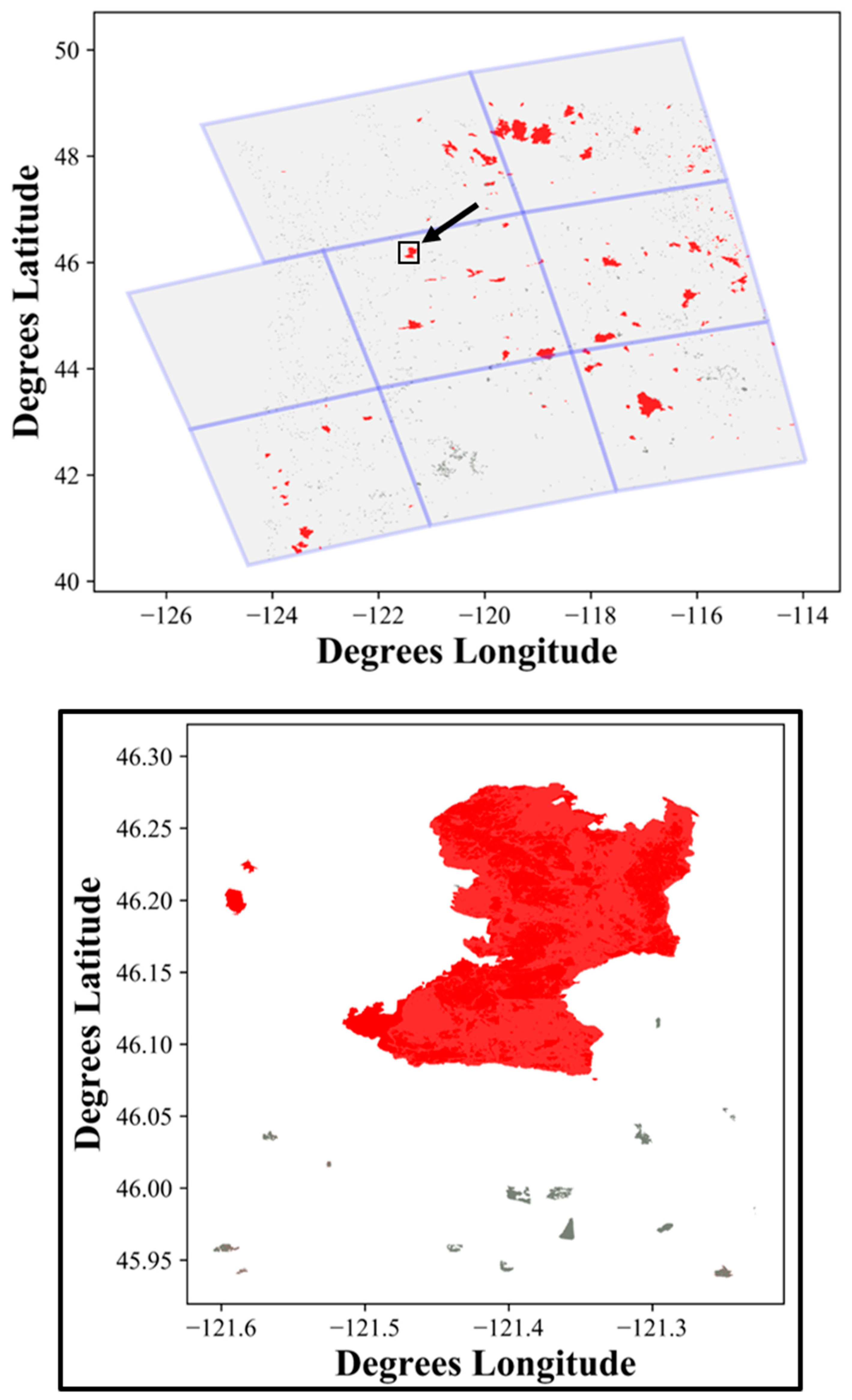
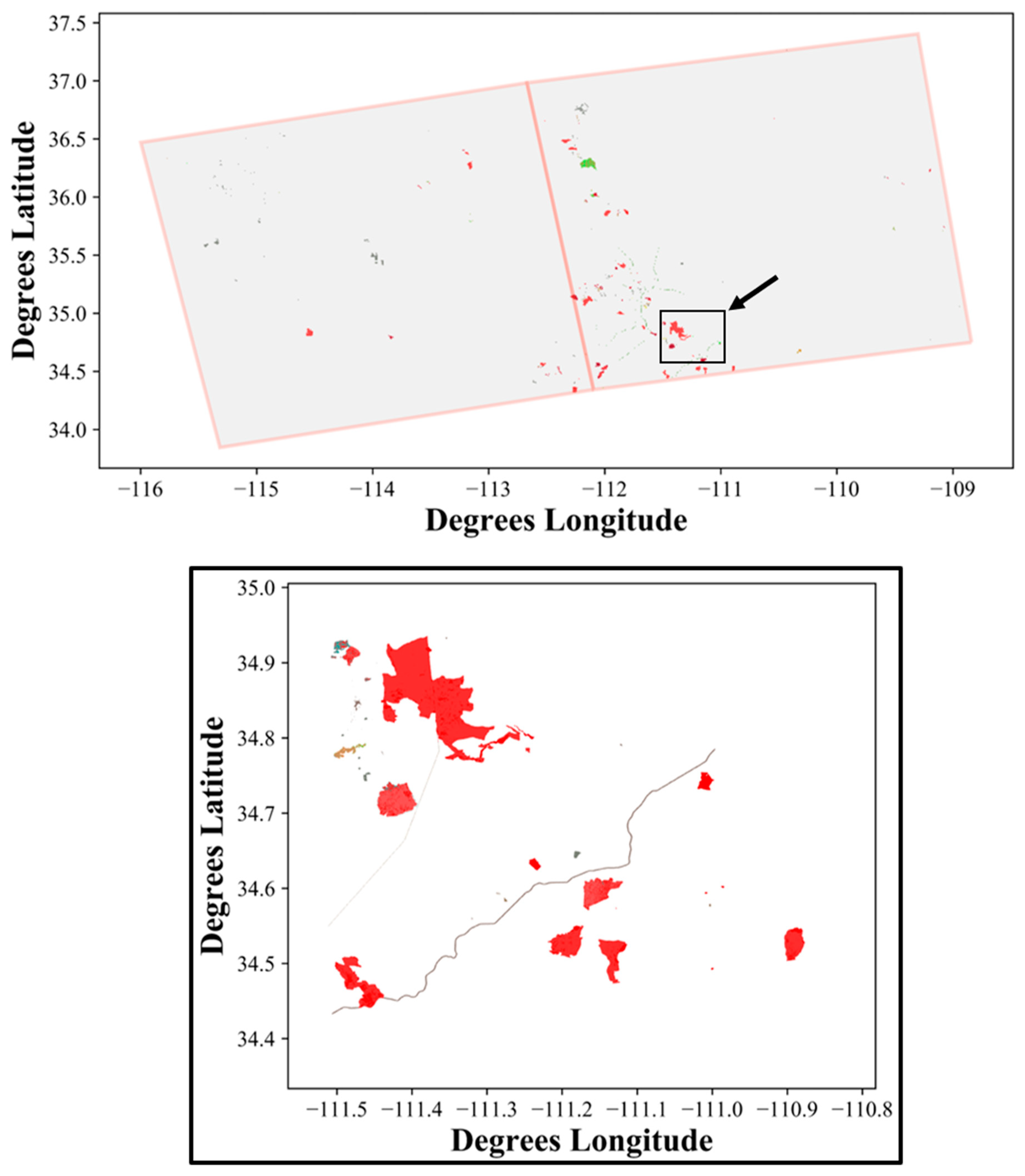
For each iteration of LANDFIRE, disturbance was classified from imagery using change detection algorithms (e.g., forest clear-cut and regeneration); from maps provided by partners (e.g., forest clear-cut and fire perimeters); and by analyst visual interpretation [5]. For disturbed areas, state and transition models were used to predict the current vegetation state of EVT and projected effects on the removal and subsequent regrowth of vegetation over time in EVC and EVH. LANDFIRE EVT, EVH, and EVC products LF 2008, LF 2010, LF 2012, and LF 2014 are therefore updated versions of LANDFIRE post-National (LF 2001).

EVT uses the Ecological Systems (ES) classification that was available at the time of LANDFIRE National [13]. As part of Remap prototyping, LANDFIRE evaluated the United States National Vegetation Classification (http://usnvc.org/, accessed 11 June 2019; NVC) as a second classification system for EVT. NVC is a vegetation classification scheme that follows the FGDC (2008; Federal Geographic Data Committee) recommendations and is composed of a nested hierarchy of eight levels [14,15]. Of these eight levels, the LANDFIRE Remap prototyping effort focused on the NVC Level 6 Group classification. The Group classification can include multiple plant species that are aggregated by a dominant growth form that is representative of a climatic, hydrologic, edaphic, and disturbance regime [15]. There are potentially 426 Groups within the United States as determined by regional experts (see http://usnvc.org/ for all classes) [16]. In this work, we focus on a subset of the Groups that occurred within the Pacific Northwest (NW) prototype area.

The aim of the LANDFIRE Remap prototyping effort is to better represent current landscape conditions (i.e., LANDFIRE base maps) based on the latest data to address known issues within the existing LANDFIRE datasets. Specifically, the LANDFIRE Remap effort will fix seam-line artifacts (i.e., abrupt transitions between vegetation classes) correlated to the input data, provide product accuracy assessments, revise product legends, address past user concerns as maintained in LANDFIRE’s database, and introduce a new NVC Group product. The efforts will result in more current base maps, independent of LF 2001 products, with all products being “remapped” from start to finish. In 2015, an initial small-scale prototyping effort was undertaken in the Clear Creek, Idaho, area to investigate new datasets and mapping methodologies [7]. The prototype area was subsequently expanded to a larger area in the NW. The majority of the Grand Canyon (GC; Arizona, USA) was later added as an additional prototype site to take advantage of extensive lidar datasets that were available. The large-scale LANDFIRE Remap prototyping effort began in summer 2016 with the overall goal to develop the foundational techniques to produce new LANDFIRE EVT, EVH, EVC, and NVC base products. The prototype was concluded one year later to kick off the Remap production effort. This paper (1) explains LANDFIRE Remap prototyping of methodologies and datasets used, (2) quantifies potential improvements in the prototype’s EVC, EVH, and EVT products over past LANDFIRE products, and (3) provides insight into the current LANDFIRE Remap production processes.

2. Materials and Methods

2.1. Prototype Areas

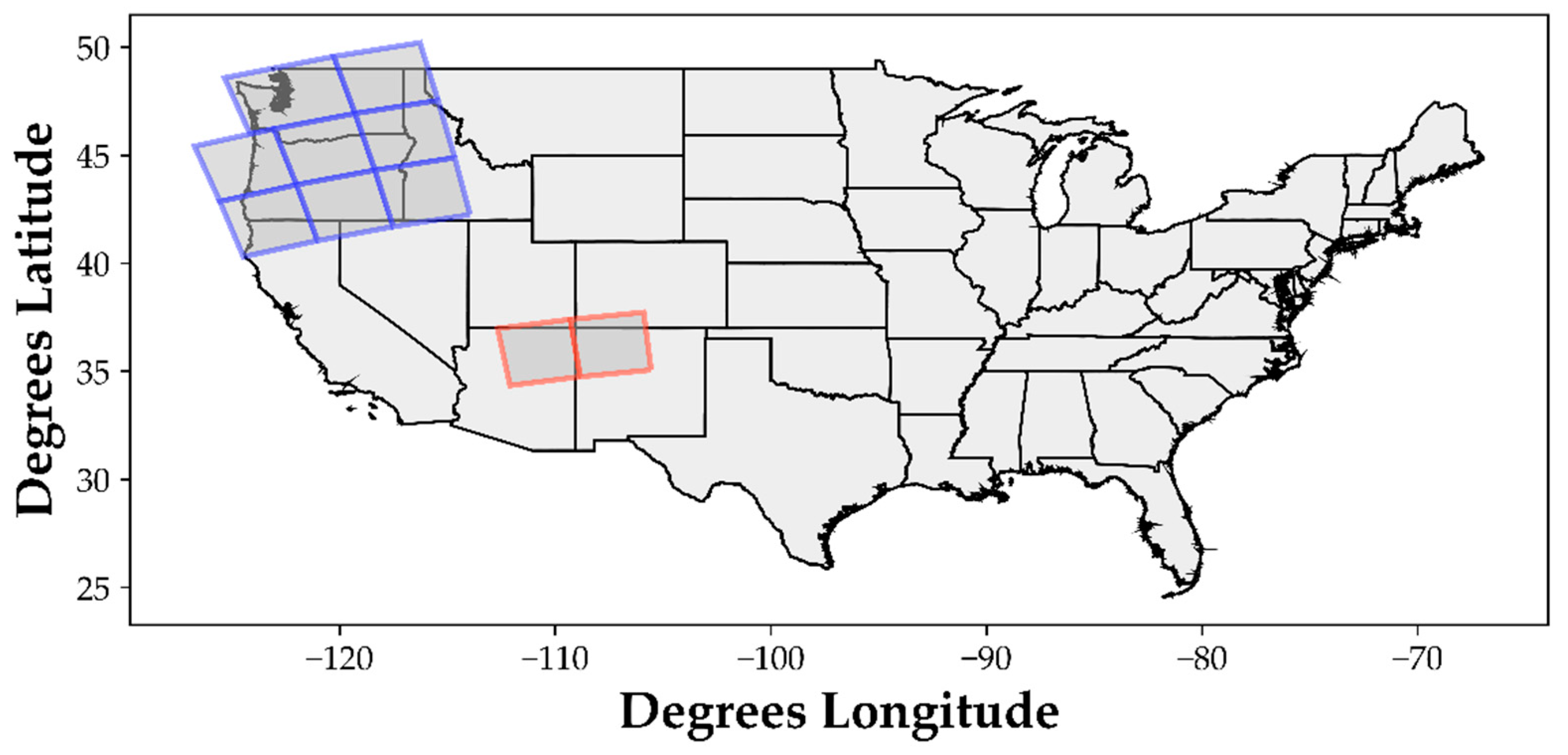
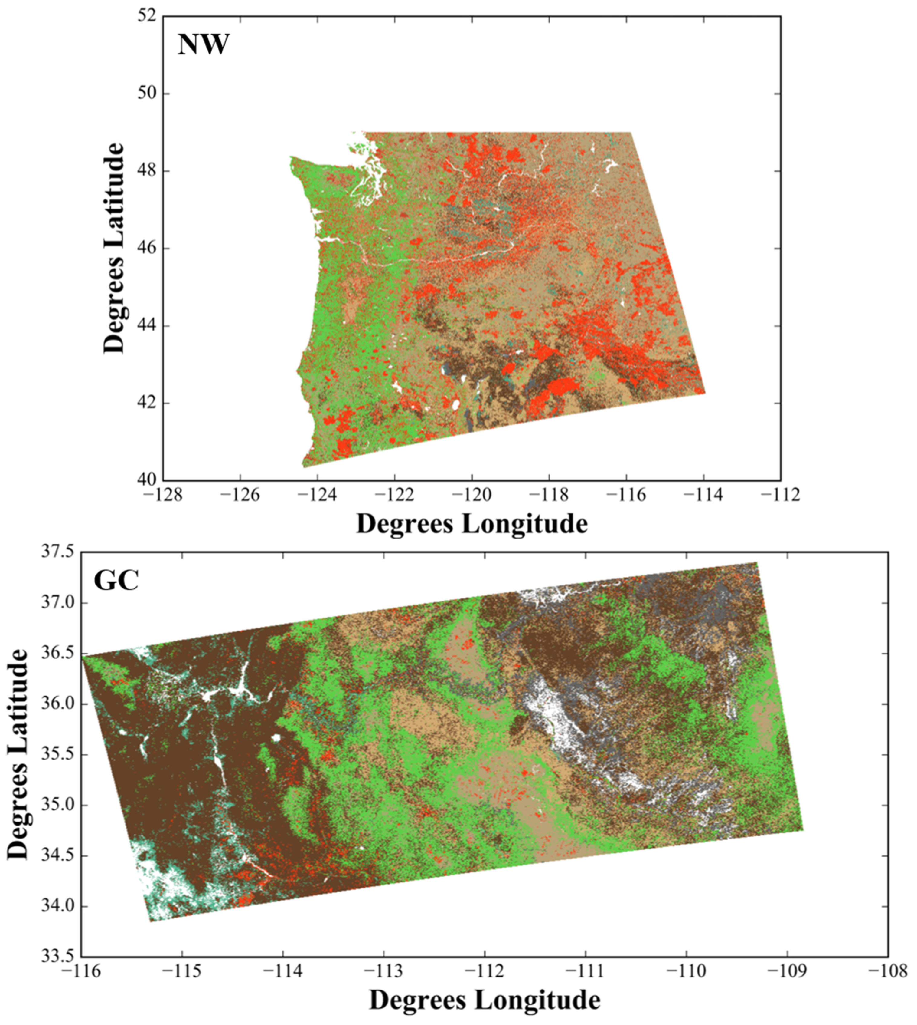
Two different geographic regions, the Pacific Northwest (NW) and Grand Canyon (GC), were examined (Figure 1). These regions were chosen for their variability in edaphic characteristics, precipitation, elevation, temperature, and vegetation conditions. The NW region includes all of Washington and Oregon, and parts of Idaho, California, and Nevada, while the GC region covers parts of Arizona, Colorado, New Mexico, and Utah (Figure 1). Elevation ranges from 0–4392 m in the NW and 21–3851 m in the GC. Precipitation varies the most widely in the NW with values ranging from 14–358 cm. In the GC, precipitation ranges from 14 to 80 cm (National Oceanic and Atmospheric Administration [NOAA] National Centers for Environmental Information, Climate at a Glance: US Time Series, Precipitation, published January 2018, retrieved on 30 January 2018 from http://www.ncdc.noaa.gov/cag/). Temperatures are highly variable in the NW, ranging from −47 to 48 °C, and from −40 to 47 °C in the GC (NOAA National Centers for Environmental Information, Climate at a Glance: US Time Series, Temperature, published January 2018, retrieved on 30 January 2018 from http://www.ncdc.noaa.gov/cag/). These large climatic ranges result in a wide array of vegetation systems within the prototyping areas.

2.2. Data Sources

Many geospatial data sources including Landsat imagery, field plot measurements, DEM, ancillary data layers (e.g., the National Land Cover Database [NLCD]), and disturbance information were used during the LANDFIRE Remap prototyping effort. While Landsat imagery and the field plot observations form the foundational datasets, other geospatial data were leveraged to improve accuracy and processing efficiency. Landsat data were corrected to surface reflectance [17,18] using the USGS Earth Resources Observation and Science (EROS) Center Science Processing Architecture (ESPA) [19] processing system (https://espa.cr.usgs.gov/, accessed 12 June 2019), reprojected to USA Albers Equal Area Conic, and resampled to 30 m. Using high-performance computing architecture, multiple Landsat scenes were stacked and ranked pixel by pixel to produce a cloud-free image composite. 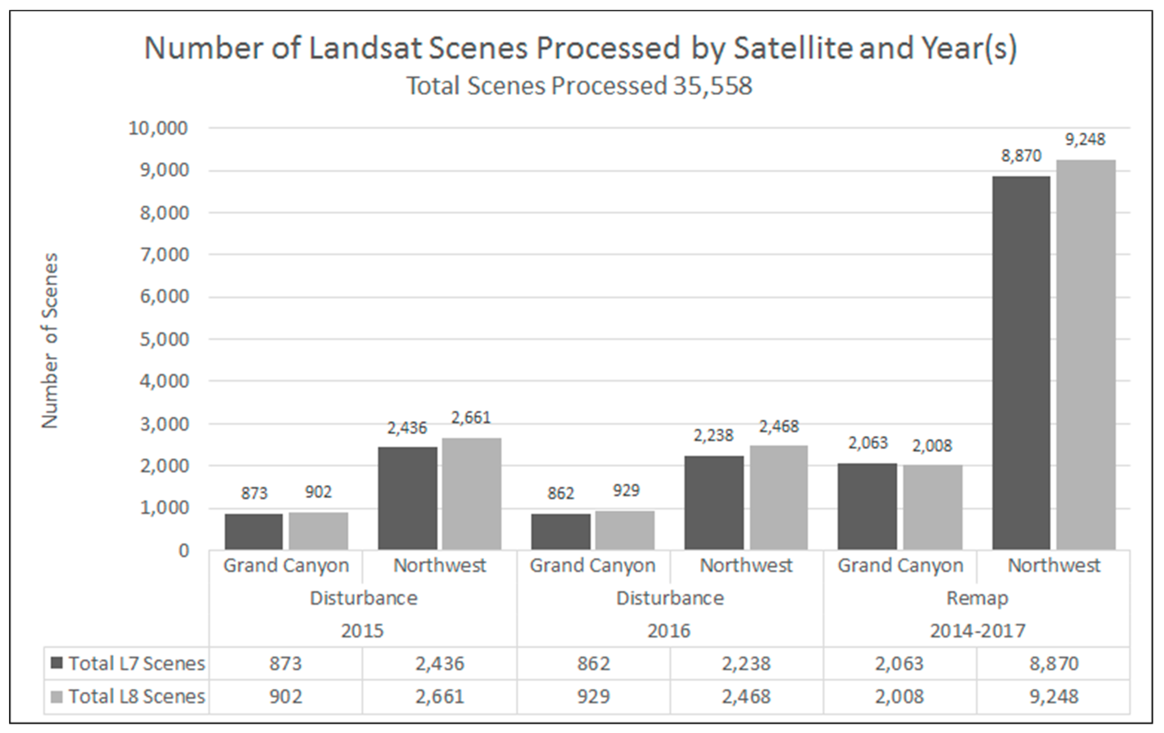This process, known as best-pixel image compositing [11], was conducted within a tiling framework covering the extent of both prototyping locations (see Figure 1 for NW and GC LANDFIRE tiles). A total of 7637 and 27,921 Landsat scenes were processed for the GC and NW, respectively (Figure 2).

Two compositing strategies were used, one for disturbance mapping and another for vegetation mapping. The first was previously developed by LANDFIRE to be used for mapping disturbance (i.e., LF 2010, LF 2012, and LF 2014) and is based upon imagery from two periods of time within the same calendar year, including early season (Julian days 135–227) and late season (Julian days 228–306) composites. Landsat imagery within the Julian date ranges is obtained from the Landsat archive (https://earthexplorer.usgs.gov/, accessed 11 June 2019) for each year of interest, placed in a virtual stack of all images, and processed to the specifications established in the best-pixel algorithm [11]. As an example, to identify disturbance in 2015, early and late season best-pixel composites are produced by year for 2014, 2015, and 2016. By limiting the imagery in each composite to a single year, each disturbance can be labeled by the year it is detected. This is important when applying transition logic to the vegetation products (e.g., time since disturbance). The disturbance composites were used to create differenced spectral indices designed for detecting change. To determine whether a change in vegetation occurred between years, the current year’s (i.e., 2015) Normalized Burn Ratio (NBR; Table 1b) values were subtracted from the previous year’s NBR values (i.e., 2014) to calculate the differenced NBR (dNBR) for both the early and late seasons. Other derivative products used for identifying change include the Normalized Difference Vegetation Index (NDVI) (Table 1b) and the Multi-Index Integrated Change Detection Algorithm (MIICA) [20].

The second compositing strategy uses imagery from a user-defined target year and the surrounding years to create a spectral composite without data gaps (areas of no data) or anomalies suited to detecting spectral differences among vegetation types. Unlike the disturbance-based composites, the vegetation composites can combine data from multiple years, which broadens the depth of available data and helps to reduce or eliminate data holes. For this prototype, the target year is 2015, so the composited imagery used for classification is referenced as circa 2015. Three Julian date ranges of imagery were chosen for compositing, including Julian days 106–178 (spring image), 179–244 (summer image), and 245–305 (fall image), to better distinguish the phenological variation in vegetation captured by Landsat spectral values due to changes in the amount of daylight, temperature, or precipitation [21]. Most pixels in the composites are from 2015, but data from 2013, 2014, and 2016 can be present where data gaps in 2015 exist.

Similar to the disturbance composites, derivative products were produced from the vegetation composite imagery, including the Modified Normalized Differenced Water Index (MNDWI; Table 1b), Modified Soil Adjusted Vegetation Index (MSAVI; Table 1b), Soil Adjusted Total Vegetation Index (SATVI; Table 1b), Tasselcap Brightness (TCbrightness; Table 1b), Tasselcap Greenness (TCgreenness; Table 1b), and Tasselcap Wetness (TCwetness; Table 1b) indices from the vegetation composite Landsat imagery. A greater number of Landsat scenes were processed for the vegetation mapping effort than for the disturbance mapping effort for the GC and the NW (Figure 2).

Additional datasets, reprojected to Albers Equal Area Conus and resampled to a 30-m pixel space, included elevation, slope, and aspect derived from DEM [22]. As with previous versions of LANDFIRE, this effort incorporated vegetation products from the National Land Cover Database (NLCD) [23], agricultural lands from the National Agricultural Statistics Service Cropland Data Layer (NASS CDL) [24], and roads and urban areas from National Transportation Statistics (http://osav-usdot.opendata.arcgis.com/, accessed 11 June 2019). The LANDFIRE 2014 Update and the Remap prototyping effort also utilized the Burned Area Essential Climate Variable (BAECV) [25] to assign the causality of possible burned areas in the disturbance product.

New datasets used for the LANDFIRE Remap prototype effort were derived from the Dynamic Surface Water Extent (DSWE) [26] product, NLCD 2016 Wetlands Potential product [27], NLCD 2011 Developed Imperviousness product [23], Level III ecoregions of Omernik [28], and watershed subbasins from a 4-digit Hydrologic Unit Code (HUC4 [29]). Furthermore, multiple airborne lidar datasets were obtained for the NW and GC Remap prototype areas to enhance vegetation structure mapping training data.

Like the LANDFIRE Refresh [4] and Update [5] efforts, the LANDFIRE Remap prototyping effort has compiled maps of natural and anthropogenic disturbances (Events) submitted by partners. Disturbance Events include national products, such as burn severity and perimeter products from Monitoring Trends in Burn Severity (MTBS) [30], Burned Area Emergency Response (BAER) [31], and Rapid Assessment of Vegetation (RAVG) [32]. LANDFIRE also receives Events data that detail date, location (i.e., polygon), and causality from federal, tribal, state, local, and private entities. Common examples of disturbance causality include fire, logging, thinning, insects, disease, and weather. If multiple Events overlap during the same year, then the event determined to be the most severe is kept as the label of causality [4].

The LFRDB is the other important dataset compiled for the prototyping effort, which has been used in all iterations of LANDFIRE products. The total number of referenced data plots assembled within the LFRDB was 100,799 in the NW and 13,246 in the GC prototype areas, of which approximately 50% have enough plant species information to be labeled with an EVT or NVC class. Important plot labels included lifeform (including barren, sparse, herb, shrub, or tree), Ecological Systems (ES) EVT, NVC Groups, percent cover, height, and geospatial location if not covered by a confidentiality agreement (e.g., FIA). Plot labels for ES EVT and NVC Groups were assigned using Auto-Keys updated for Remap [13].

2.3. Mask Development

We created binary masks to assist in the mapping process of vegetation classes that were difficult to model or control where they were mapped in a final product (see Section 2.6). Binary masks were developed for Level III ecoregions, alpine systems, water, barren areas, sparsely vegetated areas, and riparian areas that leveraged the previously mentioned ancillary datasets. The simplest binary masks to create were the Level III ecoregion binary masks. LANDFIRE National had previously used the MRLC Consortium mapping zones as binary modeling masks [22]. During the Remap prototyping effort, we determined that the MRLC map zones were too coarse for mapping EVT groups (unpublished data), which do not occur throughout the entirety of the mapping zone, resulting in errors of commission. Level III masks were therefore developed to restrict the mapping of EVT classes to specific ecoregions. LANDFIRE tiles were intersected with each Level III ecoregion, and a binary mask was then created for each tile and ecoregion resulting in 40 binary masks for NW and nine masks for GC.

An alpine mask was created to help restrict the mapping of alpine EVT classes to alpine areas in the NW prototype area. One DEM per prototype area was binned into 100-m elevation increments. This elevation class raster was intersected with HUC4 subbasins and Level IV ecoregions to develop unique classes of elevation subbasin and ecoregion. The resulting classified data were then intersected with GAP alpine vegetation classes. If a given subbasin ecoregion unit was found to be more than 25% alpine GAP classes it was coded as 1, while all other units less than 25% alpine GAP classes were coded as 0.

To create a binary water mask (i.e., water or non-water), all 2013–2015 DSWE Essential Climate Variable products were acquired for a total of 4071 in GC and 18,188 in the NW. The DSWE algorithm uses several spectral and slope tests to determine the likelihood of water presence per pixel [26]. Wherever a pixel was mapped as high confidence water (value = 1) in the DSWE products more than five times during the 5-year period, the pixel was coded as water in the water mask. We used a threshold of five because of some commission errors in DSWE products, mostly in dark non-water areas such as lava beds, non-masked cloud shadows, and within urban areas. A subsequent 3 × 3 pixel neighborhood dilation function was then used to connect potential water in neighboring pixels. Because this dilation function may add commission errors to the water mask, the summer Landsat vegetation composite MNDWI, MSAVI, and SATVI values were assessed to determine whether the dilated pixel should be labeled as land or water. If not water, then the dilated pixel’s value was changed to 0.

The creation of riparian masks for NW and GC prototyping areas required that we identify where wetlands occurred within valley bottoms. We subsequently developed a sampling methodology to extract proportional numbers of riparian and nonriparian values from the NLCD 2016 Wetlands Potential product [27]. A pixel was considered riparian (value = 100) for the sampling schema if its NLCD 2016 Wetlands Potential value was greater than 3 and not riparian (value = 0) for all Wetlands Potential values less than 3. A total of 10,000 pixels (riparian and nonriparian) were then extracted for independent values of the training data, based on the representative proportion of riparian and nonriparian pixels. The same pixel locations of three seasons of vegetation Landsat composites reflectance and Tasselcap derivatives and slope values were then extracted as independent values for the model. Training datasets were modeled within the regression tree package, CUBIST, with committee models [33] to create a continuous product with values ranging from 0–100. This modeled riparian product was subsequently thresholded, with values ≥5 considered to be riparian (value = 1) and all values <5 considered to be nonriparian (value = 0). This thresholded riparian product was compared to the DEM slope derivative to remove potential riparian commission errors. If the thresholded riparian product was near an area with a slope of 0 (i.e., the valley bottom), the final riparian mask was given a value of 1. All other values in the riparian mask that did not meet this logic were set to 0.

2.4. Disturbance Mapping Process

Disturbance mapping relied mainly on the Landsat, Events, and LFRDB datasets, and was run separately for each tile (Figure 1). As in previous iterations of LANDFIRE, the prototyping process used the Events data to determine where change occurred. Like LF 2014, MIICA [20] was used to identify areas where disturbances may have occurred. The MIICA algorithm identifies areas of spectral changes between pre- and post-year images for 2014 and 2015, respectively. Because MIICA has omission and commission errors associated with the process [20], LANDFIRE mapping analysts have developed processes to remove incorrectly identified change by the MIICA algorithm using pre- and post-disturbance Landsat imagery [5]. This entire process was time-consuming and required multiple iterations of editing to capture all disturbances correctly within the GC and NW LANDFIRE tiles (Figure 3 and Figure 4).

Once all Landsat-detected disturbances were mapped, causality was assigned by intersecting each disturbance pixel with the following datasets ordered by precedence: (1) MTBS, (2) BAER, (3) RAVG, (4) Event, and (5) BAECV. If a disturbance did not intersect any of these datasets, then the causality was labeled as unknown. Additionally, the severity of each disturbance was assessed in one of two ways. First, if a pixel fell within an MTBS, BAER, or RAVG disturbance, it was assigned to the respective MTBS, BAER, or RAVG burn severity value. The remaining disturbed pixels were assigned to a low, moderate, or high severity class by examining the mean and standard deviation value of the early and late growing season dNBR images (

Table 2. Decision logic for labeling the low, moderate, and high severity classes when severity was not assigned by the BAER, RAVG, or MTBS reference datasets. Values for each pixel dNBR value (x_pixel) was assigned by comparing it to the LANDFIRE tile-wide mean (µ_tile) and standard deviation (σ_tile) dNBR values.

Severity Class	Severity Value	Decision Logic
Low	1	xpixel < µtile + 2σtile
Moderate	2	xpixel ≥ µtile + 2σtile and xpixel < µtile + 3σtile
High	3	xpixel ≥ µtile + 3σtile

). Whichever severity image (early or late) had the highest severity value for a disturbance pixel, that severity value was used. All undisturbed areas were given a severity value of zero.

2.5. Lifeform, EVC, EVH, and EVT Data Selection and Modeling Processes

During the preliminary testing phase of Remap in the Clear Creek, ID, area [7], we tested machine-learning algorithms for the categorical modeling of lifeform and EVT classifications including random forest, k-nearest neighbor, and support vector machines within the Python scikit-learn module [34] and See5 with boosting [35], and continuous classifications (i.e., regression) for EVC and EVH including random forest, k-nearest neighbor, and support vector machines within the Python scikit-learn module [34] and CUBIST with committee models. In all classifications, only Landsat values were used as independent modeling variables. For lifeform and EVT classifications, See5 with boosting was superior in classification accuracy in Clear Creek, ID. Random forest was slightly better in prediction accuracy for EVC and EVH classification than CUBIST with committee models, but differences in accuracy were minor and CUBIST models were applied faster. We therefore decided to use See5 with boosting for categorical and CUBIST with committee models for continuous classifications, described in the subsequent sections.

The LFRDB plot locations were used to perform extractions on all geospatial input data layers for the NW and GC prototype areas. The plot extractions were performed by FIA personnel to ensure that the geospatial location of any sensitive plot dataset was not revealed. Each plot was labeled by the extracted geospatial dataset’s value and subsequently uploaded into the LFRDB. All data contained within the LFRDB could then be used for modeling lifeforms, vegetation classification (i.e., EVT), and structure (i.e., EVC and EVT).

Prior to modeling, LFRDB plots were filtered based on several criteria. First, plots without adequate information to be assigned a lifeform or EVT classification were removed from the modeling data pool. Then, barren and sparse plots were set aside for a subsequent modeling process. Plots that occurred within areas that had been disturbed within the past 10 years, and therefore were presumed to be spectral outliers, were removed using past LANDFIRE annual disturbance products and the expected recovery period for a given vegetation type. Remaining plots were then subdivided by their lifeform category, including herb, shrub, or tree. Finally, a spectral filtering test was used to compare the individual plot sum (x) of all Landsat bands (b) values (ranging from 1 to n) to the sum (V_sum) of the mean (µ) and twice the standard deviation (σ) of all plot Landsat values sampled (N):

$$x={\displaystyle \sum }_{i=1}^n{b}_i$$

(1)

$$\mathsf{\mu }= \frac{{{\displaystyle \sum }}_{i=1}^N{x}_i}{N}$$

(2)

$$\sigma = \sqrt{\frac{{\displaystyle \sum }{\left(x-\mathsf{\mu }\right)}^2}{N}}$$

(3)

$$V_{sum}= \mathsf{\mu }+2\sigma$$

(4)

If the value of x (Equation (1)) was greater than V_sum (Equation (4)), the plot was discarded from the analysis. Discarding plots using this methodology reduced the number of plots that had spectral outliers for herb, shrub, and tree lifeform types.

This “cleaned” lifeform training dataset was then used as an input for decision tree models using See5, with lifeform as the dependent variable and Landsat bands as the independent variables. Models were run over the entirety of the NW and GC prototyping areas. Once lifeform classified products were completed, they were visually reviewed with high resolution imagery from GoogleEarth for accuracy. Where areas of herb, shrub, and tree were misclassified, additional training data were digitized from high resolution data and the models were rerun. Several iterations of adding analyst-derived plot data to the training data and running the modeling process occurred until most lifeform classifications visibly matched the lifeform patterns on GoogleEarth. Occasionally, some areas of lifeform were impossible to model correctly. For these rare instances, areas of herbs, shrubs, and trees were manually digitized and recoded to the correct lifeform class.

A similar filtering process was performed for EVT vegetation type training data. Plots that occurred within areas that had been disturbed within the previous 10 years were removed if the expected recovery period for a given vegetation type had not been reached. Each EVT vegetation classification, except for barren and sparse classes, was examined by the spectral filtering test to remove spectral outliers per EVT type. Note, however, that a plot that might have been removed for modeling during the spectral filtering portion of the lifeform data cleaning process might be used as part of the EVT modeling process. As in the lifeform spectral test, the sum of individual Landsat bands per plot (Equation (1)) was compared against the V_sum (Equation (4)) values. EVT plot data were further subdivided by their Level III mapping zone and lifeform to model similar vegetation systems against each other. EVT plot labels within each Level III ecoregion were reviewed to ensure the plots occurred within the correct EVT range of distribution. Mislabeled plots either were ignored or relabeled with an appropriate EVT designation if a one-to-one crosswalk existed. A total of 10% of all plots per EVT type (i.e., test datasets) were withheld from the modeling process for an error analysis within the GC prototyping area at the end of the mapping process. Riparian, alpine, and barren or sparse EVT types were mapped separately using the binary masks developed for each. Non-riparian and non-alpine EVT classes were also modeled separately from the rest of the EVT datasets.

Each training dataset had EVT as the dependent variable and Landsat bands and DEM derivatives as independent variables. EVT classes were modeled using the See5 (with boosting) decision tree modeling software package. A total of 119 EVT types were modeled in the NW and 46 in the GC.

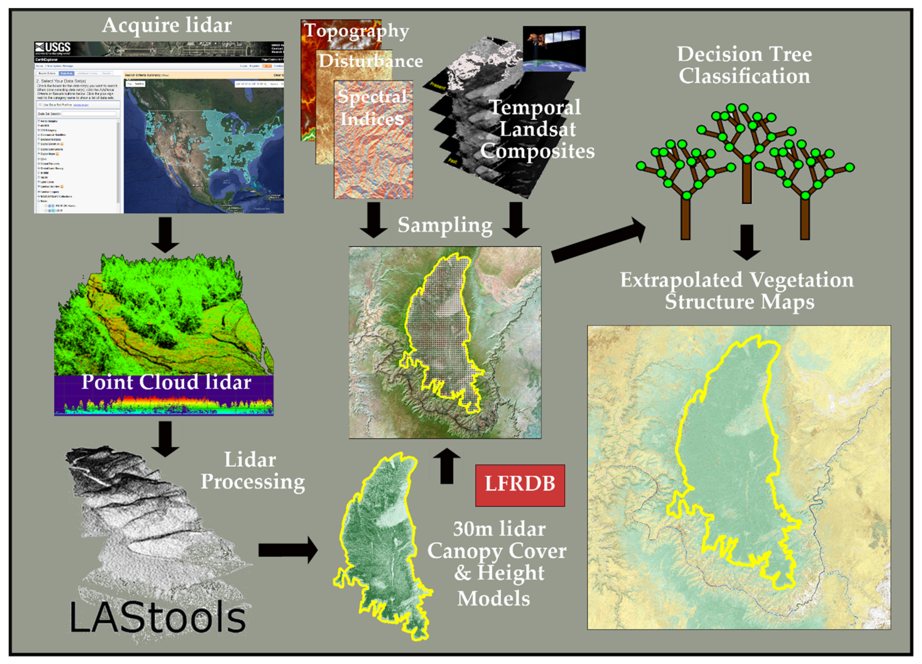
After examining the distribution of the values of canopy cover estimates of plots within the LFRDB (see Figure 4 and Figure 5 (left images) in [36]) it was determined that additional observation derived from airborne lidar acquisitions should be included to improve the thematic distribution of EVC values (Figure 4 and Figure 5 (right images) in [36]). For Remap prototyping, we developed a process by which lidar observations were combined with LFRDB plot data to develop the training dataset used to model EVC and EVH structure characteristics (see Figure 4 in [36]). First, an inventory of lidar data was performed to access lidar availability from open source resources such as EarthExplorer (https://earthexplorer.usgs.gov, accessed 11 June 2019) and OpenTopography (www.opentopography.org, accessed 11 June 2019), as well as US state distribution sites. Lidar datasets were then acquired and processed from point clouds (i.e., .las or .laz format) to 30-m canopy cover and height raster images (.tif format) using LAStools software (http://rapidlasso.com, accessed 11 June 2019). These grids were then spatially sub-sampled to build a set of lidar observations that represented the full range of lifeform cover and heights per LF tile at discrete locations in proportion to their occurrence. Next, independent variables, including Landsat composites, vegetation spectral indices, and topography composites, were extracted against LFRDB plots and lidar-derived observations to create training data required for CUBIST committee decision tree classifiers. Lidar and reference plots that fall within recently disturbed areas were discarded from the training dataset. Finally, decision tree models were used to create EVC and EVH products (Figure 5).

We found that incorporating lidar data increased the amount of EVC reference data by 310% in the Grand Canyon and by 79% in the Northwest prototype areas. The addition of lidar data increased reference data in areas that are under-represented by the LFRDB reference plots alone; for example, tree cover ranging from 10% to 15% had very few plots in the NW and GC reference plots; however, including lidar considerably increased the plots in this range, as well as in most other percent cover classes.

2.6. Merging Datasets

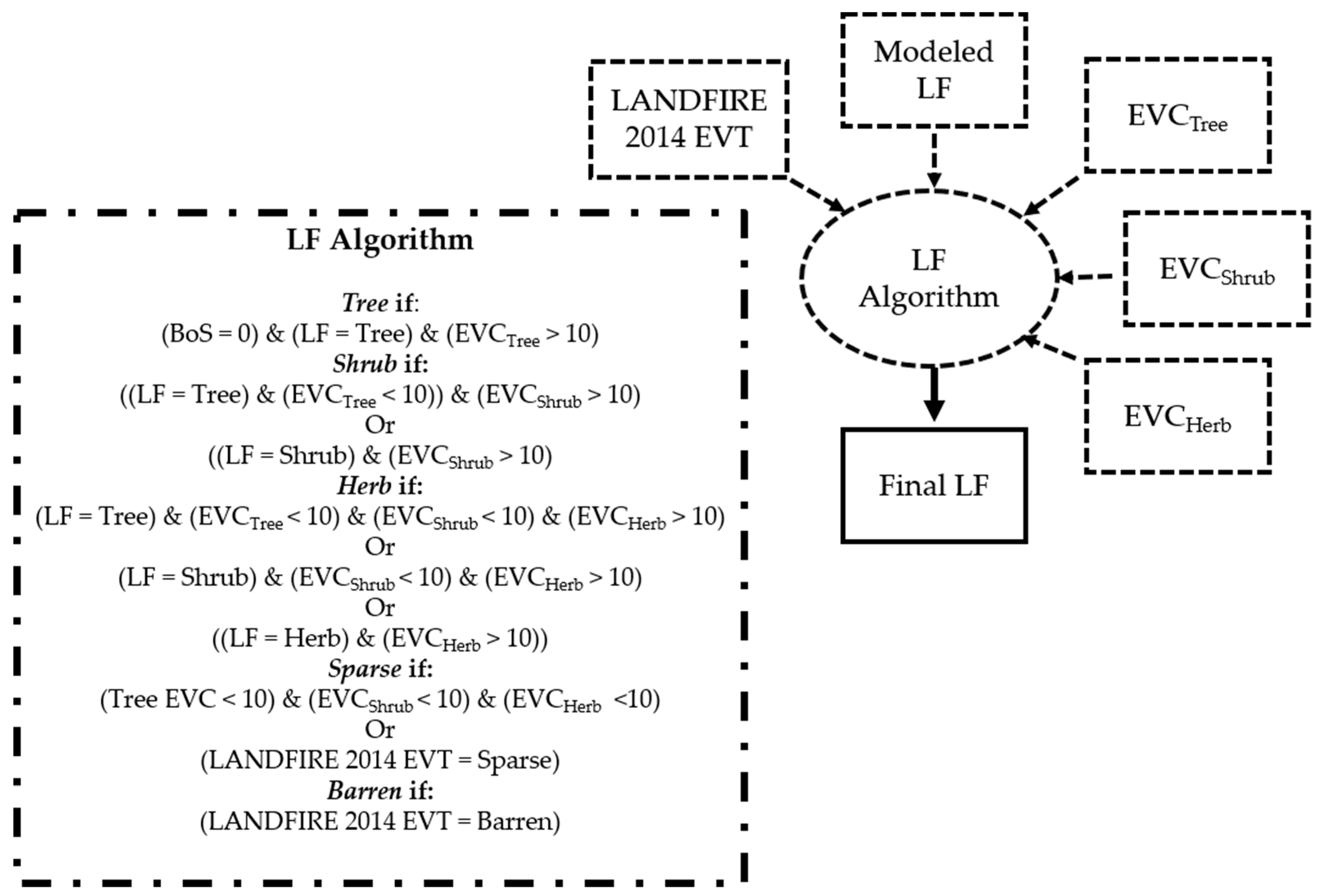
After all components for lifeform, EVT, EVH, and EVC datasets were completed, processes were developed to put the pieces together for the NW and GC prototype areas and generate the final maps (Figure 6). For compatibility, all datasets needed to be able to nest within the lifeform layer. The first step in the merging of data products was to create a complete lifeform map. This was done by first modifying lifeforms by EVC lifeform layers on a per-pixel basis, as follows. If a given pixel was classified as a tree within the lifeform layer, and the tree EVC percent cover layer was >10%, then the lifeform class remained classified as a tree; however, if the tree lifeform class was <10% cover in the EVC dataset, then shrub and herb EVC layers were examined following the same logic as previously mentioned for the tree EVC layer to determine whether the lifeform class should be shrub or herb. If all the EVC lifeform classes had <10% cover, the lifeform classification was labeled as sparse. Finally, barren and sparse pixel designations in LF 2014 were added to the final lifeform product.

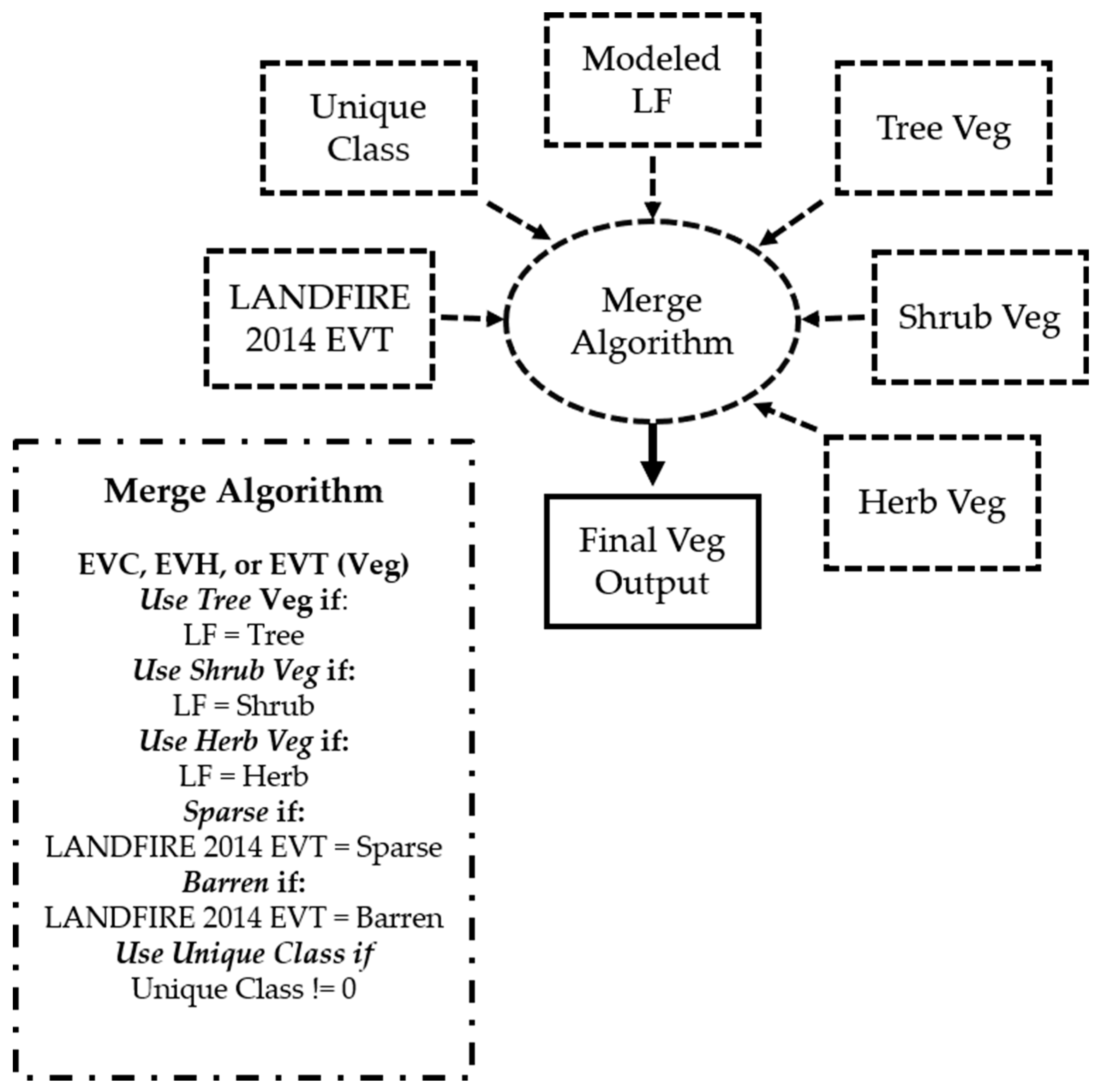
This newly revised lifeform layer was then used to merge EVC and EVH model runs together for both prototype areas. Individually modeled EVH lifeform layers were merged by their lifeform type and recoded (Figure 7). For example, a tree lifeform pixel would be assigned a tree EVC value. Unique values of EVC ranged from 0–400, with 0–100 reserved for indicating unique codes (e.g., water (value 11), barren (value 31), and sparse (value 100)); tree pixels were coded as the sum of 100 and the percent tree cover, and shrub pixels were coded as the sum of 200 and the percent shrub cover. Herb pixels were coded as the sum of 300 and the percent herb cover. For example, an EVC of 127 would represent a forested pixel with 27% tree cover. EVH was coded by lifeform similar to EVC, except for replacing percent cover in the summation with height in meters, decimeters, and centimeters, respectively, for tree, herb, and shrub. Both EVC and EVH therefore indicate lifeform by their respective 100, 200, and 300 classification value. Additionally, the classes including water, barren and sparse, urban, agriculture, and mines were added to the map from the masks described above.

EVT data were compiled into one image per prototype area by using the lifeform layer to merge all the different model runs together by lifeform and specific modeling run by mask (Figure 7). These included the separate models for Level III, riparian, alpine, and sparse vegetation areas. Additional vegetation classes were burned in, including disturbance with lifeform and water from the DSWE.

NVC groups were cross-walked with EVT instead of modeling, to test out the process’s feasibility within the NW. No additional model runs were conducted for riparian, alpine, or sparse vegetation. Additional disturbance and water classes were burned in as mentioned previously for EVT.

Previous studies have found that object-based image analysis (OBIA) segmentation processes that group nearby spectrally similar pixels together into objects can improve vegetation classification when compared against traditional pixel-based approaches [37]. To determine whether the OBIA segmentation approach might improve the classification of EVT, all Landsat bands were used within eCognition [38,39] to develop classification segments. These segments were then used to determine the most common lifeform present (i.e., majority) per segment, resulting in a segmented lifeform classification map. Separate tree, shrub, and herbaceous EVT majority segment maps were then developed based on the previously modeled EVT classifications. The segmented lifeform map was then used in conjunction with the three separate EVT maps, one map of all EVTs categorized by tree, shrub, or tree lifeforms (e.g., tree EVTs), to compile one segment-based EVT map. Disturbances and water classifications were not segmented but were instead used “as is” from the disturbance and water maps.

2.7. Error and Comparative Analyses

Lifeform was assessed for similarity by comparing the NW and GC prototype to the LANDFIRE 2014 Update. The overall idea was not to assess whether the Remap prototyping effort produced a more accurate product than LF 2014, but to ascertain how lifeform pixels changed between the two iterations of LANDFIRE. Disturbances that occurred between 2014 and 2015 could change the lifeform between the years. To deal with this potential problem, we removed all pixels that were disturbed in either 2014 or 2015. Additionally, all barren and sparse classifications were not considered in this analysis. To compare the two products, the overall area (hectares) per lifeform class that stayed the same or switched classes (e.g., tree to shrub) was calculated.

To ascertain whether including lidar data improved EVC and EVH values in the GC prototype area, the tree LFRDB-only, lidar-only, and combined modeled outputs were compared to withheld FIA plot data (N = 38). A simple linear regression was created with the withheld tree percent cover and height (m) from the FIA plot data versus the modeled output, and the goodness of fit (R²) was assessed.

The EVT product for the GC prototype area was assessed by comparing the values of the stratified randomly withheld values (10% by type with a minimum training data sample size of 30) with the produced EVT values in the GC prototype area. An error matrix was constructed to compare the expected vegetation classification from the LFRDB to the modeled output (

Table 3. Potential error matrix that calculates the agreement between a LANDFIRE-mapped vegetation product and withheld field-validated plots contained in the LANDFIRE Reference Database (LFRDB) for different vegetation classes ranging from vegetation classification 1-N (Veg1-VegN), where N indicates some number of vegetation classifications. Cell agreement between the LFRDB and modeled product are highlighted in gray.

Mapped	LFRDB
	Veg1	Veg2	VegN
Veg1	Veg1/Veg1	Veg1/Veg2	Veg1/VegN
Veg2	Veg2/Veg1	Veg2/Veg2	Veg2/VegN
VegN	VegN/Veg1	VegN/Veg2	VegN/VegN

). Conventional accuracy assessment metrics including overall (OA), producer’s (PA), and user’s accuracy (UA) were then calculated [40,41].

3. Results

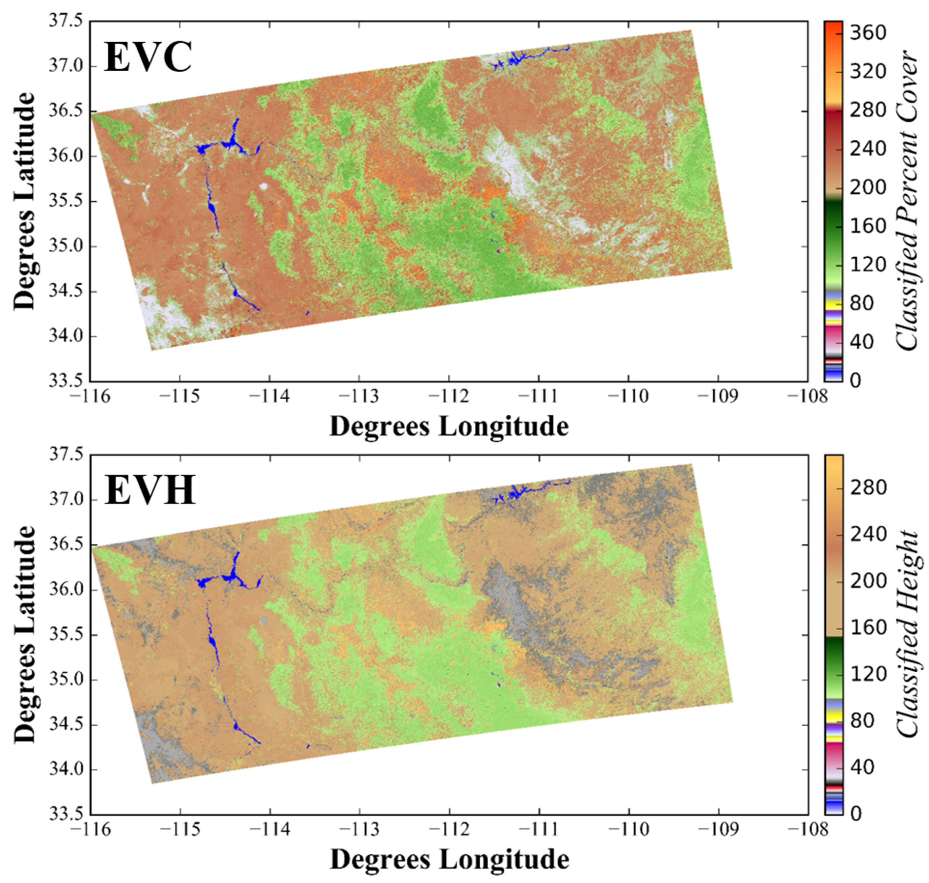
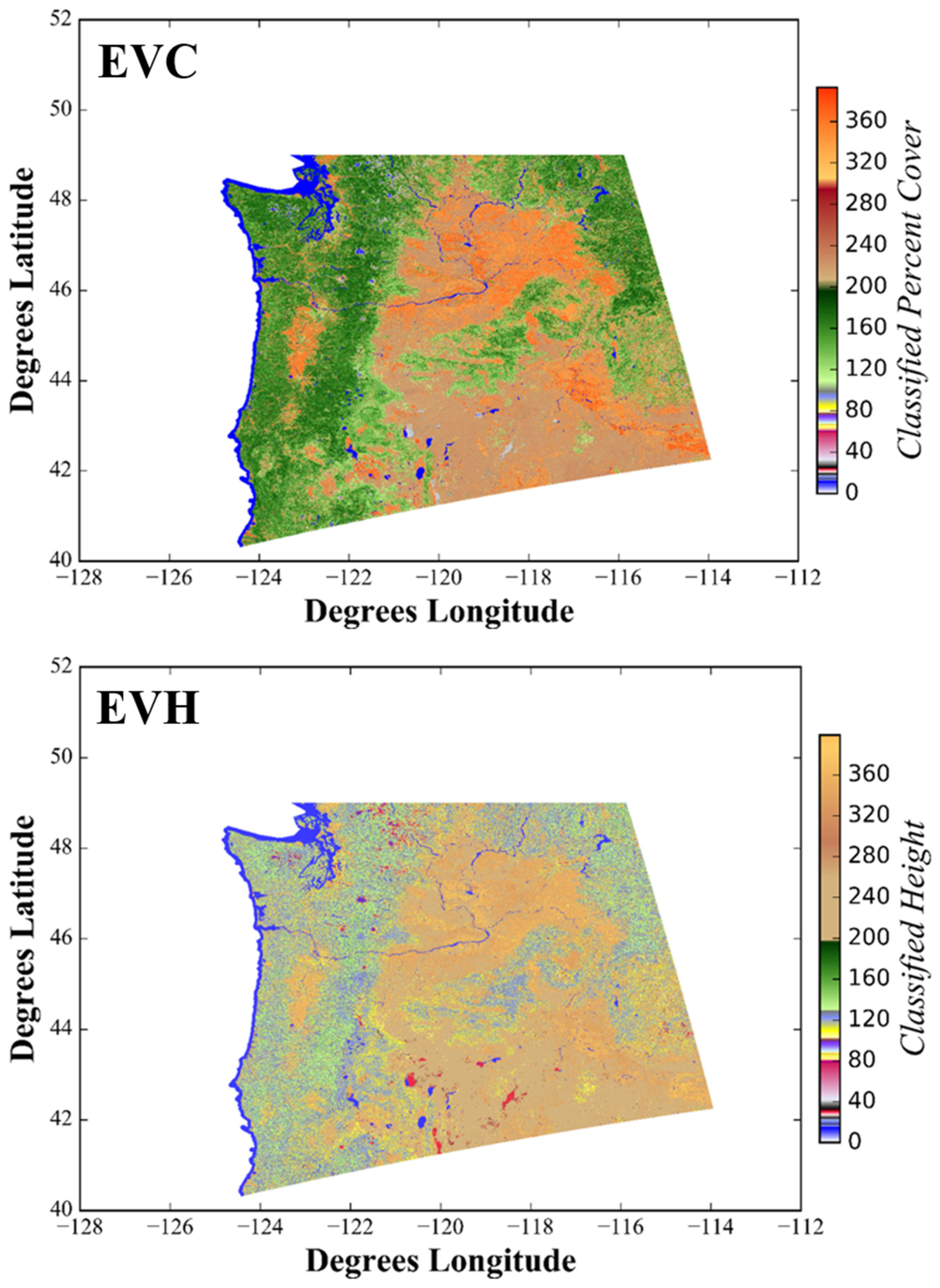
NW and GC prototype maps for EVC, EVH, and EVT (Ecological Systems and Groups) were successfully produced for the LANDFIRE prototype effort (Figure 8, Figure 9, Figure 10 and Figure 11). EVC and EVH products are classified products; however, they feature much finer thematic resolution than previous versions of LANDFIRE (Figure 8 and Figure 9). The EVT thematic products feature a total of 150 and 55 classes for the NW and GC prototype areas, respectively. The NVC Group thematic product had a total of 81 classes within the NW (Figure 11).

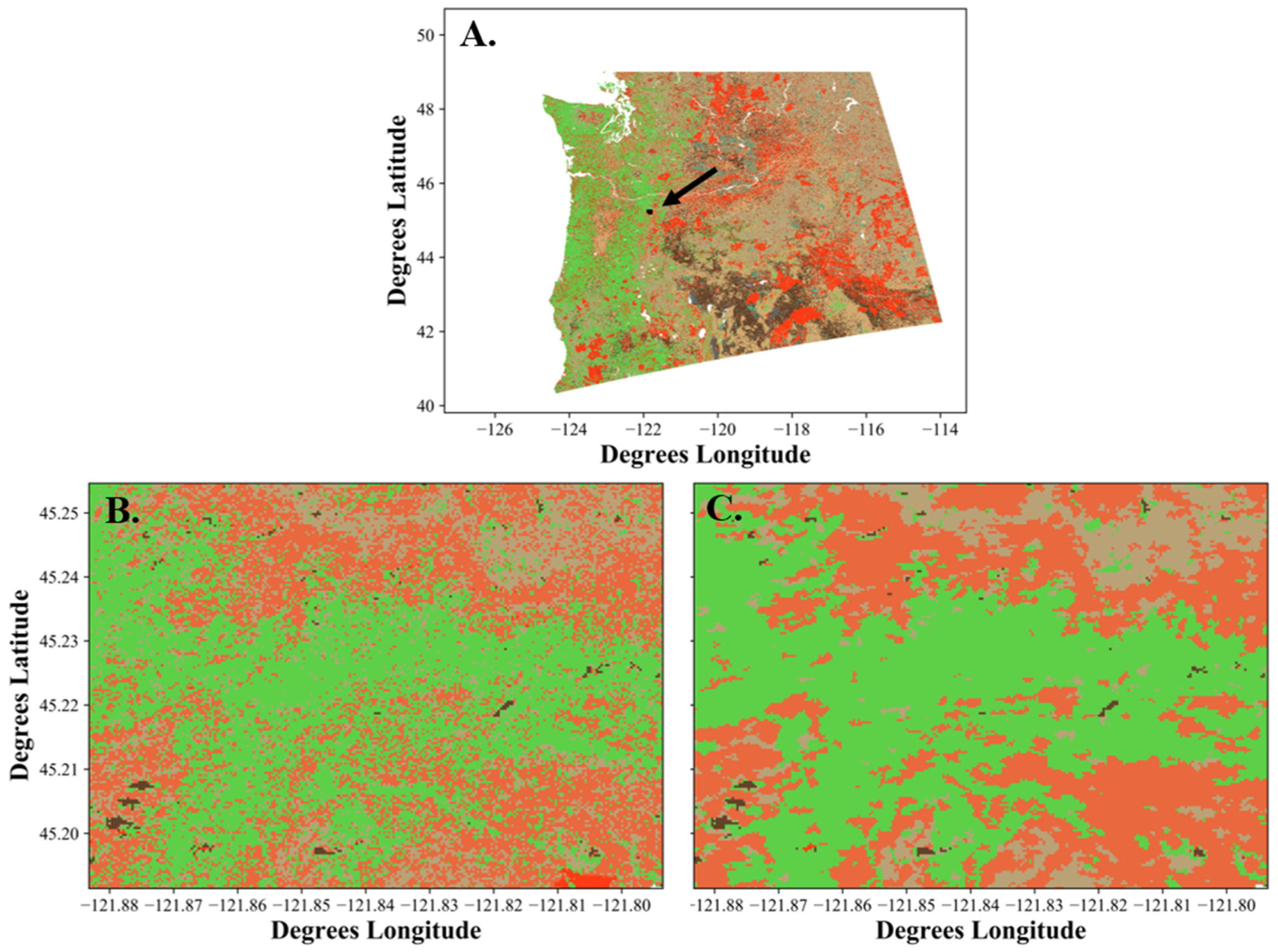
A segmented EVT map (Figure 12A.) was produced in addition to the original EVT map (Figure 10, left) for the NW. Differences in pixilation are evident when the EVT (Figure 12B.) map is compared to the segmented EVT map (Figure 12C.) for a portion of the NW, with the segmented map exhibiting reduced pixilation. Segmented EVT maps required an order of magnitude more processing time for production.

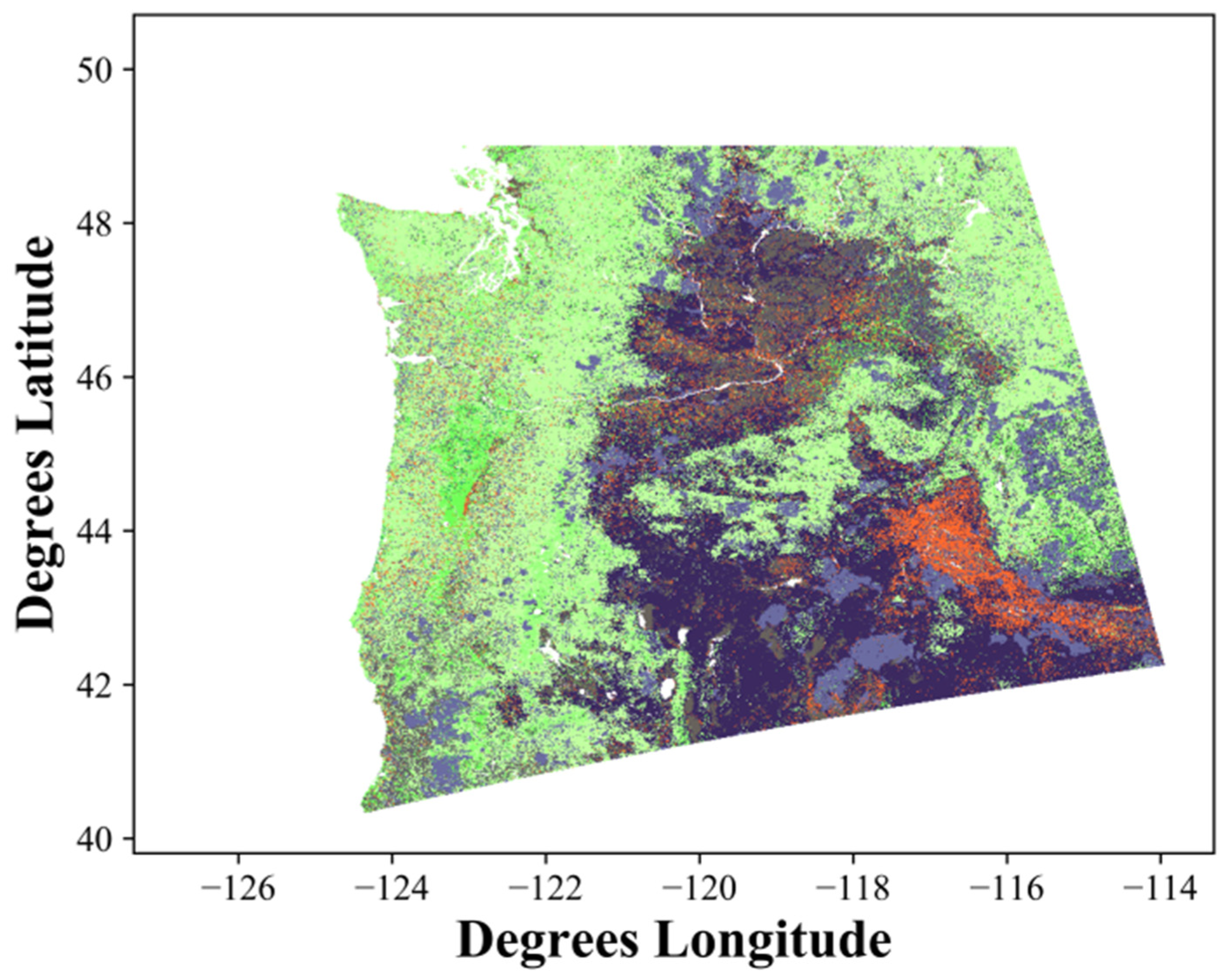
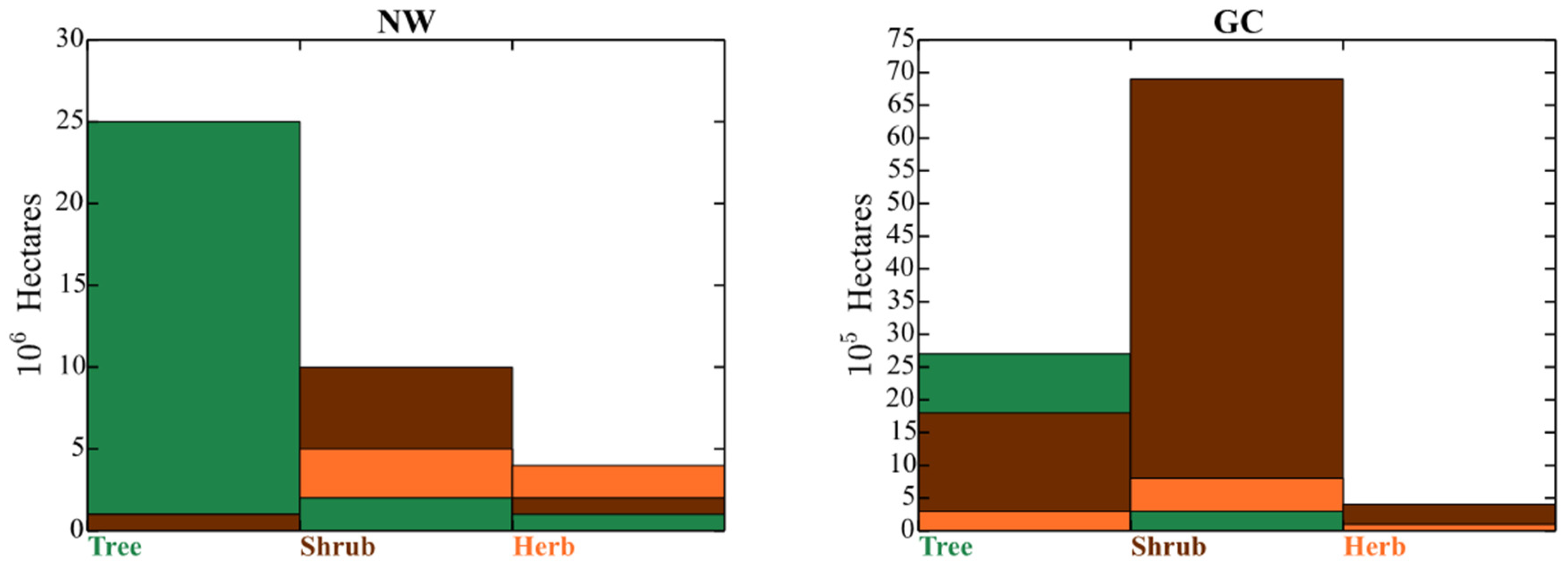
Lifeform pixel classifications differed between the LF 2014 and Remap prototyping effort within the NW (Figure 13). Trees were the dominant vegetation classification (26.43 × 10⁶ hectares), followed by shrubs (17.03 × 10⁶ hectares) and herb classifications (7.23 × 10⁶ hectares). A total of 3.42 × 10⁶ hectares of pixels switched from shrub and herb classes to tree. More herb pixels changed (1.93 × 10⁶ hectares) to shrub than tree (0.79 × 10⁶ hectares) to shrub. Shrub (4.88 × 10⁶ hectares) pixels were more likely to change to herb than tree (0.82 × 10⁶ hectares) to herb.

Differences between the LF 2014 and Remap were also evident in the GC (Figure 13). The order of composition of the vegetation classes was shrub (7.99 × 10⁵ hectares), tree (4.74 × 10⁵ hectares), and herb (0.622 × 10⁵ hectares). A total of 0.31 × 10⁵ hectares classified as shrub and 0.04 × 10⁵ hectares of herb in Update switched to tree in Remap. The shrub class was much reduced in Remap, with 0.80 × 10⁵ hectares converting from herb in Update. A smaller fraction of the tree pixels (0.31 × 10⁵ hectares) converted to shrub. Finally, more herb pixels (0.45 × 10⁵ hectares) were classified as shrub in LF 2014 than herb (0.14 × 10⁵ hectares) or tree (0.04 × 10⁵ hectares).

Moderate fits between the modeled percent cover of the LFRDB-only, lidar-only, and combined data modeled outputs compared to withheld FIA plot percent cover were evident (see Figure 7 in [36]). Merged LFRDB and lidar percent cover datasets resulted in the best goodness of fit (R² = 0.51), although goodness of fit with lidar-only data was not dissimilar (R² = 0.49). LFRDB-only models led to the worst fit (R² = 0.43).

Like percent cover, the LFRDB-only data modeled height map exhibited the worst fit (R² = 0.04) when compared to FIA plot height (see Figure 8 in [36]). The lidar-only modeled height map had the best relationship with FIA height data (R² = 0.57). When LFRDB data were combined with lidar, the fit of the modeled height dataset decreased compared to the lidar-only modeled height dataset (R² = 0.53).

In this analysis, 55 EVT classes were assessed for the GC prototype area (Figure 10), making error matrixes difficult to view within a standard table. Please see Supplementary Materials S1 and S2 for the full error matrix and summary of errors, respectively. The overall accuracy of all mapped classes was 52% (Supplementary S1). Of the classes with >20 plots (N = 14) of withheld data (accounting for 81% of all withheld plots), user’s accuracies ranged from 29%–83%, and producer’s accuracies ranged from 5%–87% (Supplementary S1 and S2). The remaining 41 classes averaged 5 plots of withheld data, generally exhibiting much lower producer’s and user’s accuracies (Supplementary S1 and S2).

4. Discussion

The LANDFIRE Remap prototype (2015) effort resulted in new large-scale vegetation cover, height, and classification datasets for the NW and GC prototype areas. The methodologies for producing these maps drew upon past LANDFIRE mapping campaigns; however, new mapping techniques were developed to take advantage of unlimited, free access to Landsat data, high performance computing, state-of-the-art mapping techniques, and unprecedented access to field and lidar data. Assessments of the NW and GC prototype areas’ data products suggest that there were distinct changes to the lifeform product compared to LF 2014. Changes to the Remap prototype lifeform and production methodologies led to subsequent changes in the EVC, EVH, and EVT products. Accuracy metrics for the EVC, EVH, and EVT products in the GC prototype area suggest that these changes have resulted in products with moderate accuracies.

It is difficult to compare the past versions of the LANDFIRE EVC, EVH, and EVT datasets to the NW and GC prototypes because the legends were altered between versions. Nevertheless, the lifeform types, into which all layers are nested, have remained consistent, allowing for direct comparisons. Our analysis showed differences within the lifeform tree, shrub, and herb classifications (Figure 13). The largest were in the GC prototype area, where 1.75 × 10⁵ hectares of the total pixels shifted from shrub in LF 2014 to tree. This change is likely due to improved strategies in assigning sparsely treed areas as tree rather than shrub. We noticed significantly more pixels correctly categorized as tree than in LF 2001. It is possible there was encroachment and successive growth of piñyon-junipers systems within the prototyping areas [42], but that is unlikely because these systems demonstrate periods of growth and die-off [43].

Another major lifeform shift was apparent in both prototype regions, where herb moved to shrub. Worth noting was the addition of EVC into the modeling process, which was a departure from LF National that potentially shifted the classification from herb to shrub. It is possible that there was some expansion of conifers into former grasslands [44], in which the conifers would exhibit shrub-like heights and coverage. Additionally, there has been post-fire conversion of shrubs to exotic herbs (e.g., cheatgrass, Bromus tectorum) within the prototyping area [45], and this conversion is projected to continue [46]. Therefore, increases in shrub cover within the prototype areas has more likely resulted from changes in classification rather than changes in vegetation between 2001 and 2015.

Improvements in overall accuracy were most significant in EVH due to the incorporation of lidar data. This makes sense considering that many data sources referenced in the LFRDB came from disparate sources and were not necessarily collected to the rigorous standards of FIA data, for example. The lidar data also give a more comprehensive sampling of the potential heights present in the entirety of the landscape, which is clearly visible in the distribution of the heights of trees visible within the LFRDB-only versus combined LFRDB and lidar datasets. What is surprising, however, is that the combined LFRDB and lidar datasets resulted in a slightly weaker relationship between the modeled and FIA data. This may be because the addition of the LFRDB data overwhelmed the contribution of the lidar dataset, and could potentially be fixed by adding more lidar data to the training dataset to better encompass the full range of distribution in tree height [47] not fully represented within the LFRDB.

As previously mentioned, direct comparisons between previous and current EVT products in this prototype area are impractical due to the altered vegetation classes. Nevertheless, general observations can be made by withholding percentage plot data and using it in an accuracy assessment. For Remap EVT, we calculated an accuracy of 52%, which was below the approximate 80% mark other large-scale vegetation products that have been exhibited [48,49,50]. However, these thematic land cover products had far fewer than the 55 classes mapped in the GC prototype area. Increasing the number of classes (i.e., map complexity) generally decreases the accuracy of a thematic map [51]. Our overall accuracy is therefore more comparable to thematic products with larger numbers of classes [52,53]. Additionally, this study leveraged data from disparate sources with varying purposes from which quality was not disclosed. Poor training data can reduce the quality of thematic maps [54], which most likely decreased our accuracy for some EVT classes. Potential training data errors are also likely exacerbated by the way in which the EVT classes are assigned via Auto-Key within the LFRDB. The Auto-key’s accuracy ranges from 36.5%–85% [13], and subsequently can have a large effect on EVT training data and model accuracy.

We applied OBIA segmentation to the pixel-based EVT product to determine if map accuracy would improve, and if a segmented product could be produced within the scope and time frame required from a national-scale production effort. Although we were successful in producing the segmented EVT product, the amount of time it took to perform the operation proved impractical for implementation for LANDFIRE Remap. Training data were not withheld; therefore, we could not assess the statistical accuracy of the segmented against the pixel-based EVT product. However, a visual comparison indicated that EVT classes were often homogenized in areas where multiple EVTs were expected. This suggests increased errors in areas where coexisting vegetation types are common (e.g., rare vegetation types occurring in small patches), as well as those that occur heterogeneously across a wide-ranging landscape [55].

This is the first time the NVC Group product has been produced for LANDFIRE. In the future, it is anticipated that a national-scale NVC will become a standard LANDFIRE product. This is important given that NVC is the federal standard classification system for the US and for all federal agencies [56]. NVC also conforms to international vegetation classification standards and is similar to the Canadian National Vegetation Classification (CNVC [16]), allowing for better cross-border vegetation mapping.

Like LF 2012–2014, Landsat composite imagery was used as the base data for all mapping efforts. However, in this prototyping effort, we mapped both disturbance and classified thematic vegetation classes, which required two sets of image composites to be produced independently of each other. Image anomalies (e.g., unmasked clouds, shadows, snow, etc.) can introduce spectral artifacts that may result in classification errors. Such anomalies are less impactful to the disturbance product because trained analysts inspect all pixels identified as change to ensure they were not caused by composite-driven aberrations. Less time was spent hand-correcting potential problematic pixels for the thematic vegetation classification image composites. Yet, an effort was made to identify and remove problematic Landsat scenes from the compositing process if deemed necessary. The danger of composite-driven anomalous pixels is potential propagation errors from lifeforms through EVC, EVH, EVT, and NVC. It is therefore advisable that additional time be spent examining the underlying Landsat image composites for the LANDFIRE Remap production effort.

All EVT mapping was conducted by using Level III ecoregions. This allowed for subdividing the landscape into smaller, more-manageable processing units. However, processing smaller scales for all vegetation classes often results in sharp breaks between thematic classes, causing seamlines at unit boundaries. To remedy this problem, we found that mapping units simultaneously can reveal seamlines, which can be corrected during the modeling process. These units could be subdivided further as necessary (e.g., Level IV ecoregions), but ecologically similar areas should be mapped together to provide continuity among mapping classes as well as a reduction of hard edges between thematic classes.

For the Remap production effort, it is important that ample time be devoted to the difficult-to-map classes. During the prototyping effort, limited time was spent post-processing and correcting modeled products. We acknowledge that additional time dedicated to improving mapping accuracies is necessary and an important part of the mapping process. For instance, by examining the automated error calculations during the draft stages of production, low-accuracy classes can be identified and improved by adding training data using “expert opinion” plots, by developing new masks to control the mapping of specific hard-to-map classes, or by hand-editing the maps.

5. Conclusions

We successfully produced EVC, EVH, EVT, and NVC LANDFIRE base maps for the NW and GC prototyping areas. The classification and error assessment methodologies presented here will be implemented in the LANDFIRE Remap 2016 production effort and automated within an open-source framework (i.e., Python [57]) to promote transparency, reproducibility, and transferability in mapping processes. These automated processes will contribute to production efficiencies and data quality improvements in both Remap and future iterations of LANDFIRE. Other benefits include decreased production costs via reductions in computer- and person-time, and, perhaps, shortened production cycles. The LANDFIRE Remap production effort has incorporated the bulk of our recommendations and automated processes with as-needed modifications to achieve the goal of producing higher quality maps while minimizing the difficulties identified in this effort.