Deriving Fire Behavior Metrics from UAS Imagery
by
Christopher J. Moran
1,*, 
Carl A. Seielstad
1,
Matthew R. Cunningham
1,
Valentijn Hoff
1,
Russell A. Parsons
2,
LLoyd Queen
1,
Katie Sauerbrey
3 and
Tim Wallace
1 1
National Center for Landscape Fire Analysis, University of Montana, 32 Campus Drive, CHCP 428, Missoula, MT 59812, USA
2
US Forest Service, Rocky Mountain Research Station, Fire Sciences Laboratory, 5775 W. Highway 10, Missoula, MT 59801, USA
3
The Nature Conservancy, Sycan Marsh Preserve, OR 97621, USA
*
Author to whom correspondence should be addressed.
Fire 2019, 2(2), 36; https://0-doi-org.brum.beds.ac.uk/10.3390/fire2020036
Submission received: 21 May 2019
/
Revised: 12 June 2019
/
Accepted: 20 June 2019
/
Published: 22 June 2019
(This article belongs to the Special Issue Unmanned Aircraft in Fire Research and Management)
Abstract
:The emergence of affordable unmanned aerial systems (UAS) creates new opportunities to study fire behavior and ecosystem pattern—process relationships. A rotor-wing UAS hovering above a fire provides a static, scalable sensing platform that can characterize terrain, vegetation, and fire coincidently. Here, we present methods for collecting consistent time-series of fire rate of spread (RoS) and direction in complex fire behavior using UAS-borne NIR and Thermal IR cameras. We also develop a technique to determine appropriate analytical units to improve statistical analysis of fire-environment interactions. Using a hybrid temperature-gradient threshold approach with data from two prescribed fires in dry conifer forests, the methods characterize complex interactions of observed heading, flanking, and backing fires accurately. RoS ranged from 0–2.7 m/s. RoS distributions were all heavy-tailed and positively-skewed with area-weighted mean spread rates of 0.013–0.404 m/s. Predictably, the RoS was highest along the primary vectors of fire travel (heading fire) and lower along the flanks. Mean spread direction did not necessarily follow the predominant head fire direction. Spatial aggregation of RoS produced analytical units that averaged 3.1–35.4% of the original pixel count, highlighting the large amount of replicated data and the strong influence of spread rate on unit size.
1. Introduction
Although laboratory and modeling approaches offer greater control of environmental conditions and better replicability than is possible in field settings, empirical studies of fire behavior remain important to a range of scientific inquires [1,2,3,4], including supporting theory of fire spread dynamics [5,6], evaluation/validation of mathematical fire models [7,8,9,10], and assessments of fire and other disturbance interactions [11,12], fuel treatment design and effectiveness [13,14,15], and fire behavior process-vegetation pattern relationships [16,17,18]. In each of these areas of study, field observations and experiments provide opportunities to quantify actual fire behavior providing validation of numerical experiments in an intellectual environment that still prefers real-world corroboration of modeling research [6,19]. Remote sensing from handheld devices, tripods, manned aircraft, satellite, and, increasingly, unmanned aerial systems (UAS), are fundamental to the systematic measurement of fire behavior in the field [20].
The most common fire behavior metrics that are derived from empirical studies can be grouped into two distinct types: (1) energy release as characterized by intensity and/or power [21] and (2) fire movement such as rate of spread (RoS), spread direction, and residence time. Measurements of fire energy have significant scientific legacy from a multitude of small-scale laboratory experiments [22,23,24], in-situ field observations [25,26,27], and regional to global assessments of satellite imagery [28,29,30,31]. Significant limitations and assumptions are inherent in the estimates of fire radiative energy (FRE), fire radiative power (FRP), and fire intensity, primarily related to difficulties in collecting data over the full temporal range of combustion [32,33,34]. However, the performance of these metrics is well-documented in the literature, and many of the caveats are well-summarized in Table 6 of Hudak et al. [35].
Derivations of fire movement metrics are less common in the literature, but they are experiencing a renaissance of sorts [36,37,38,39]. Fire RoS, an essential metric for characterizing fire intensity [40], and more generally fire behavior, has become obtainable at high temporal and spatial resolutions (~0.1–1 Hz and 1–50 cm, respectively) from UAS. The ability of UAS to collect data from new perspectives and variable scales has created a need for more robust algorithms to characterize fire progression and RoS. Such fire movement data are increasingly valuable for characterizing relationships between fire behavior and environmental patterns in fuels, moisture, wind, and topography, as well as in providing better estimates of fire intensity and real-time data for managing wildfires.
UAS confer a fresh, dynamic, and relatively safe and inexpensive perspective for studying wildland fire in field settings [4,41,42]. A rotor-wing UAS hovering above a fire provides a static, scalable scientific measurement platform, with some advantages over other systems. For example, fixed-wing aircraft must be moving, and thus face challenges in providing spatially and temporally consistent measurements [39]. Helicopters have the same hovering capabilities with longer flight durations [36,43,44], but they come with high operating costs, complex logistics, increased risk, and the potential to produce rotor wash that affects fire behavior. Boom lifts [27], towers [45], large tripods [46], or trees can raise sensors to overhead perspectives but constrain the spatial extents of measurement and must be resistant to high temperatures.
There has been growing interest in the capabilities of UAS as a fire research tool, but their limitations are still not widely known [41]. Hardin et al. [47] outline the six primary challenges to using UAS for environmental remote sensing. Relatively short flight times (~10–30 min) for small rotor-wing UAS is the primary challenge and it largely determines mission parameters, such as launch and landing locations and the amount of time for uninterrupted data collection. Payload limits restrict sensor weight and, often as a result, sensor performance capabilities (e.g., uncooled microbolometers vs. cooled shortwave thermal cameras). Visual line-of-sight rules limit operating extents in many locations and further constrain launch and landing locations [41]. Consequently, pilots, visual observers, and researchers are constantly at risk of interfering with fire operations. UAS operations have not yet been fully integrated into fire operations either, and most fire personnel have little experience working with UAS when compared to traditional manned aircraft [48]. All of these factors increase the operational complexity in an already complex fire environment. Deploying UAS in prescribed fire settings simplifies operations somewhat compared to operating in uncontrolled wildfire situations, enhances research efficacy, and exposes scientists and fire managers to strengths and weaknesses associated with UAS use more broadly.
UAS are also proving useful for collecting vegetation data, resulting in opportunities for acquiring coincident fuels-fire behavior datasets with increasingly finer grains and larger spatial extents. Relatively cheap UAS hardware combined with structure-from-motion photogrammetric techniques can be used to build detailed three-dimensional (3-D) models of the environment [49,50,51]. Lidar systems, which are being mounted to UAS platforms, have also produced 3-D datasets of similar quality and detail [4,52]. Thus, the analysis of pattern-process ecological relationships is now possible in unprecedented detail and extent. There are at least two major and interrelated concerns for these types of pattern-process analyses. First, the size of analytical units becomes an important consideration [3]. Point cloud data are often summarized over two-dimensional (2-D) pixels or 3-D voxels with a number of metrics that characterize the arrangement or presence/absence of points over defined areas or volumes [52,53]. The choice of area or volume of these units can significantly affect results [54]. Secondly, and specific to study presented here, the estimation of fire movement suffers from a lack of data between consecutive images. This can lead to a violation of statistical assumptions, particularly sample independence, and thus the determination of appropriate analytical units is necessary.
Fire has inherent spatial and temporal dependence as a self-perpetuating chemical reaction [55], which should be accounted for or leveraged in analyses. In particular, for RoS, if the values are attributed to individual pixels at the original resolution of the imagery, interpolation is necessary between flame fronts locations. These are essentially redundant data introducing artificial spatial autocorrelation (SA), which confounds the true SA signal. This effect is spatially variable, as missing data increases when fire covers a larger area between images (i.e., higher RoS). Statistical inference and model performance will undoubtedly be affected by inflating independent sample sizes (i.e., pseudo-replication) and the aforementioned confounding of the true SA signal [56]. This general issue is coined the ‘change of support problem’ or ‘modifiable areal unit problem’ (MAUP), where ‘support’ refers to the geometrical size, shape, and spatial orientation of the region associated with the value or measurement of interest [57,58].
Here, in conjunction with estimating fire spread metrics from UAS imagery, we introduce a method to derive more robust analytical units, while also maintaining inherent SA, in order to improve pattern-process analyses, such as fuel-fire behavior interactions. Our approach is methods-oriented with the intent of sharing techniques in sufficient reproducible detail, and with the expectation that fire research with UAS will continue to develop and expand in use. Our paper addresses the following specific objectives:
- Collect spatially and temporally consistent images of free-burning fire using UAS-borne thermal IR, NIR, and visible cameras on spatial domains of 0.01–1 Ha.
- Generate image time-series with known radiometric and geometric fidelity.
- Extract fire progression, rate of spread (RoS), and spread direction in complex fire behavior (e.g., interacting fire lines, multiple heads) using automated methods.
- Determine appropriate analytical units from fire behavior data to improve statistical analysis of fire-environment interactions (e.g., fire behavior-fuels).
- Share lessons-learned with the intent of flattening the learning curve for others adopting UAS technology for wildland fire operational and research use.
2. Materials and Methods
The following methods were derived from UAS deployments on a dozen prescribed fires in the states of GA, FL, MT, and OR, USA. Here, we focus on data collected from seven field plots in three prescribed fires conducted in dry ponderosa pine forests of western MT and southern OR. Five plots were located at the University of Montana’s Lubrecht Experimental Forest (referred to as Lubrecht henceforth) in May 2017. Two plots were located at The Nature Conservancy’s Sycan Marsh Preserve (Sycan henceforth) in October 2018. Plot dimensions for the Lubrecht experiments were 10 × 10 m. The Sycan experiments expanded plot sizes to 100 × 100 m. Data were collected by positioning a UAS with nadir-viewing cameras above plot center and imaging fire as it burned through a plot. We include relevant background and literature pertinent to the specific methods below.
2.1. UAS Platforms and Sensors
After testing many rotor-wing UAS and sensors (e.g., platforms: DJI (Shenzhen, GD, China) Phantom, Phantom Pro, M600, M100; Skyfish (Missoula, MT, USA) M4; ICI (Beaumont, TX, USA) Halo; 3DR (Berkeley, CA, USA) Solo, X8 (DIY); GoPro (San Mateo, CA, USA) Karma; sensors: FLIR (Wilsonville, OR, USA) XT; ICI 8640; ICI SWIR 640; DJI X3, X5; Sony (Tokyo, Japan) A7R, QX1, QX30, A6000; GoPro Hero; MicaSense (Seattle, WA, USA) RedEdge), we selected the DJI Matrice M100 with a dual battery configuration and the FLIR XT and MicaSense RedEdge sensors. The Matrice provided reliability at relatively low cost along with a good balance of size, speed, hovering stability, flight time, payload, software capability and stability, camera integration, availability of spare parts, and ease of repair. A bench-calibrated (prior to both field missions) FLIR XT thermal camera (7.5–13.5 µm spectral band) mounted on a DJI gimbal was used for the Lubrecht experiment. A multispectral Micasense RedEdge camera on a fixed mount (no gimbal) was added for the Sycan burns. These two sensors provide multispectral, radiometric assessment of fire and vegetation at wavelengths of 0.465–0.86 µm and 7.5–13.5 µm. Table 1 shows the sensor specifications.
2.2. Plot Selection and Layout
Eight ground control points (GCPs) were established at the corners of two nested squares for each plot. At Lubrecht, the outer square had 10x10m dimensions with the inner square at one-third the area (3.33 × 3.33 m). For Sycan, the outer squares were 100 × 100 m and the inner squares were 10 × 10 m. The internal geometry of the GCPs was established with measurements from a TruePulse laser rangefinder. GCP locations were geotagged using an Emlid Reach RS rover-base station dGPS setup. Plot layout and UAS camera orientation were consistent to ease interpretation and georectification of imagery. Plots were selected to minimize canopy occlusion but also to represent a variety of western US surface fuels that typically experience low and mixed severity fire. Plots were ignited using a drip torch with the intention of achieving a coherent, steady-state fire front spreading perpendicular to a plot edge. In practice, heterogeneous fuels and shifting wind speed and direction led to ignitions at variable distances and directions from plot edges. For example, fire in Sycan plot 1 failed to carry into the plot, and it had to be re-ignited in receptive fuels within the plot boundaries.
2.3. Data Collection
The UAS hovered at a fixed altitude above plot center with cameras viewing nadir. Table 1 reports the flying altitudes, corresponding pixel sizes, and other relevant data collection parameters.
Flight altitudes were established to capture the extent of the plot with a buffer of 2–5 m at Lubrecht and 10–15 m at Sycan. Data were collected for at least one UAS battery cycle, until active fire spread within the plot ceased, or progression of fire operations necessitated travel to the next plot. Temporal resolution was fixed at 0.2 Hz at Sycan and 1 Hz for Lubrecht, although image capture rates were delayed to 0.13 Hz and slightly variable (SD of 0.13 s) at Lubrecht due to memory card issues. The FLIR XT was the primary sensor for the Lubrecht burn. Both the Micasense RedEdge and FLIR XT were used at Sycan although the RedEdge was the primary camera for RoS derivation.
2.4. UAS Imagery Stabilization and Georectification
An important consideration for deriving useable fire data from UAS is the stabilization of imagery to mitigate platform drift and jitter [59]. Gimbaled sensors reduce these effects, but correction is still necessary. The first step is to establish GCPs that can be identified in different spectral bands with fire in the field of view. Either ‘cold’ (i.e., low emissivity) or ‘hot’ (usually charcoal beds) targets relative to background temperatures are options. After extensive experimentation, we settled on low-emissivity, 40 × 40 cm polished aluminum targets (for Sycan) and 12 cm diameter aluminum foil-wrapped circular targets (for Lubrecht), which proved to be reliably identifiable in visible and infrared imagery. Target visibility was tested at multiple altitudes in sunlit and diffuse lighting as well as in active fire conditions.
Two basic methods were evaluated to create co-incident, georectified imagery: (1) georectification alone, which effectively corrects image jitter while rectifying, but requires each image to be separately processed and (2) image stabilization of the time series, followed by separate georectification. Georectification alone may seem faster, but automated GCP and tie-point locators struggle with the rapid change between images due to fire spread. This created the need for manual identification of GCPs and other visible tie-points in every individual image necessitating significant time and resources. GCPs were also obscured by fire and smoke in some images, which led to inconsistent results across the time series. The use of image stabilization algorithms, specifically those designed for video stabilization, resolved these issues [59]. We used the warp stabilizer algorithm within Adobe After Effects (version 15.1.2) for this purpose, although open-source variants are also available. By locating objects that are relatively invariant throughout a time-series or only using the previous image to identify tie-points, image stabilization algorithms efficiently produce image stacks that need GCPs to be visible in only one image (often pre- or post-fire) for effective georectification. The downsides of video stabilization techniques are their tendency to transform data to into video compliant data types (8 or 16 bits), which often involve data scaling.
2.5. Data Pre-Processing
Before calculating fire behavior metrics, aligned imagery was converted to radiance (Micasense RedEdge) and radiant temperature (FLIR XT) and organized in raster stack form. The FLIR XT sensor requires proprietary software to extract radiometric data and calculates radiant temperature based on calibrated equations specific to the sensor. Although improvements in radiant temperature estimates can be made using a set of user inputs, the inputs can be temporally and spatially variable (e.g., emissivity) [60] and subject to radiometric saturation. Thus, accurate spatial calibration is unlikely. We used default values besides ambient temperature and relative humidity, which were measured at take-off for each plot. An emissivity constant of 0.98 was utilized. Calibration of imagery from the Micasense RedEdge is integrated into several software packages (e.g., Agisoft Metashape), although its use for observing fire requires customized scripts. A GitHub webpage provides Python scripts and tutorials [61]. The RedEdge camera has five distinct sensors for each spectral band, and the image rasters must be aligned post collection. While Micasense provides an automated alignment script, the results proved inconsistent. We used the GCPs to create an alignment model using an affine transformation within ERDAS Imagine software (version 16.5.0) to achieve satisfactory band-to-band alignment. We then followed Micasense’s algorithms for radiometric calibration and calculation of radiance for each spectral band.
2.6. Flaming Combustion Determination
Characterizing the movement of flaming combustion begins with a definition of flaming, as measured by the sensors employed. Most commonly, raw digital numbers from the sensor are converted to radiance and then transformed to radiant temperature. A static threshold is then applied to the radiant temperatures for a binary classification. The value of this temperature threshold varies considerably in the literature from 150 °C [44], 326.85 °C [36], 426.85 °C [43], 499.85 °C [38,40], and the Draper point at 525 °C [62]. Another approach is to define the flaming front using edge detection algorithms, which rely on gradient change in the imagery [37,45,63]. Major advantages of edge detection approaches are the ability to apply them to image data that do not have robust radiant temperature transformations available and in situations where absolute values of radiance may be affected, such as smoky atmospheric conditions. With the rapid development of UAS-specific sensors, we prefer the gradient approaches, as datasets are likely to be variable in scale, resolution, and sensor-specific parameters, such as spectral bands and sensitivity. Theoretically, one gradient-based approach could be applied to a variety of imagery and yield similar results, whereas methods reliant on radiant temperature thresholds would likely have to be customized for each sensor and perhaps for different spatial resolutions as well.
However, gradient-based approaches typically define only the leading flame front edge. As the active flame front is often discontinuous and complex in heterogeneous fuels, the edge-smoothing needed to account for gaps, such as in Ononye et al. [63], simplifies subsequent fire behavior calculations and risks reducing the variability seen at the fine scales capable from UAS perspectives. Additionally, fire spread into areas not ignited by the initial flaming front will often be ignored in these gradient-based approaches.
To overcome the limitations of both methods, we combined temperature threshold and edge detection techniques to maintain observed variability and to maximize indifference to resolution, sensor, and spectral band differences. First, edge detection following the Canny method was applied to each thermal image [64]. Valero et al. [37] showed that the Canny method discriminates between the flaming front, transient flames, and pre-frontal heat. Instead of directly using these edges, we extracted pixel values along the defined flame front edge from the Canny algorithm and applied a two class k-means clustering algorithm to automatically determine the flaming combustion threshold [65].
From one perspective, determination of flaming combustion (and any binary classification) requires optimizing the balance between errors of commission (false positives) and omission (false negatives) [66]. Errors of commission are abundant in the pixels that immediately precede the flaming front due to preheated fuel and soot particles. Errors of omission are high in situations with high RoS, low residence time, or occlusion by vegetation or smoke. In our study, for example, areas of sparse grass and litter overlaying rock burned quickly but also cooled quickly once the flame front passed. This required logic to attribute pixels that clearly burned in the flaming front but were never detected above the flaming combustion threshold (omission error). Similarly, if temperature thresholds are set too high, omission error rates increase leading to erroneously discontinuous flaming fronts. In such cases, fire spread direction loses coherency, and estimates of RoS will erroneously decrease. Alternatively, low thresholds cause high rates of commission error, which increase RoS, reduce variability in spread direction, and incorporate unburned pixels.
We tested a dual-threshold approach to account for these situations: one to define the leading edge weighted towards a low error of commission and another weighted to minimize error of omission. This approach allows for the use of data from one or multiple sensors and a single spectral band or a split window using different spectral bands. In our experiments at Sycan, we erroneously acquired data from the FLIR-XT in the high-gain setting for plot 1, which saturated the pixels at 190 °C. This plot also had the grass-overlying-rock fuel arrangement causing the residence times to be shorter than the temporal resolution of the imagery. We thus used the Micasense NIR (0.82–0.86 µm) radiance values to define the leading flame edge through Canny gradient detection and k-means clustering. Within each particular timestep polygon, any pixels that did not reach the threshold were then compared to the FLIR XT data. If at the lower threshold (190 °C), the pixels were assumed to have experienced flaming combustion at that particular timestep. A single threshold was applied as defined by the k-means clustering for the other plots (Lubrecht plots 1–5 and Sycan plot 2), since the residence times were consistently longer than the temporal resolution of the imagery.
2.7. Fire Progression
Each pixel in the time-series stack was assigned the timestep at which flaming combustion initially occurred after a temperature threshold was applied individually to each image. This is termed a fire progression or time-of-arrival data layer, which is the basis for all subsequent fire behavior calculations presented in this study.
2.8. Spread Rate and Direction
Of all the metrics based on fire movement, RoS and spread direction may have the most utility for characterizing fire behavior. RoS can be estimated in the field, is commonly used, and exerts strong influence on the estimation of fire intensity [40]. Johnston et al. [38] showed that sensor and algorithm choice have significant influence on these estimates. Regardless of how flaming combustion is determined, the most popular approaches to estimate RoS utilize vector contours with movement speed and direction estimated from straight lines perpendicular to adjacent contours. In cases where threshold temperatures are used, contours are derived from the progression map, while edge detection approaches inherently create contour vectors. Often, the flaming front is broken and discontinuous and steps are needed to reduce the resulting complex geometry of the resulting vectors. Paugam et al. [36] found that areas of complex vector shapes were difficult to characterize and had to average groups of pixels at the cost of losing data by increasing pixel resolution to 1.44 m from the initial 18 cm. Valero et al. [59] and Onyaye et al. [63] smoothed the contours and applied logic to traverse flame front gaps in order to create continuous vector lines.
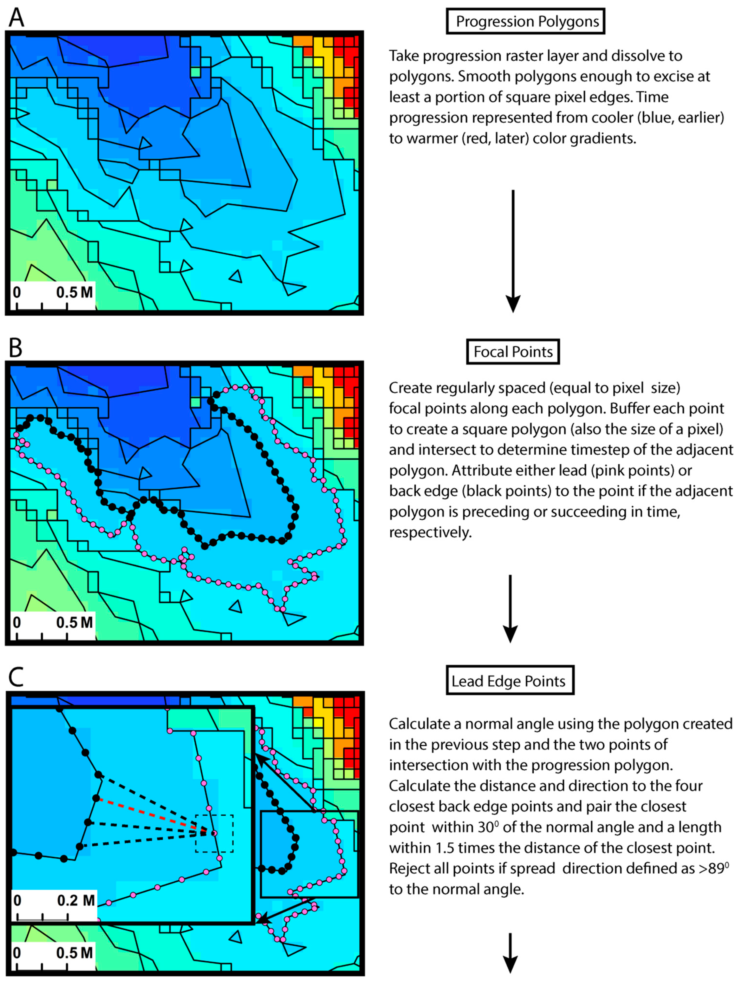
Our perspective was to characterize the variability and complexity observed in wildland fire settings and to compliment the diversity of imagery that can be collected with UAS. We formulated a new algorithm building on the previous work discussed above. While we utilize UAS-derived imagery, the approach could be applied to nearly any overhead, coincident time-series imagery. We explicitly consider complex fire behaviors, such as multiple distinct firelines interacting, which are common in heterogeneous fuels typical of western US forest ecosystems. The approach is primarily vector-based relying on pairing points defined as lead (i.e., where the fire is heading) or back edge (i.e., where the fire came from). Figure 1 illustrates the algorithm. Scripting was completed using R statistical software [67], with the additional packages ‘raster’ [68], ‘sp’ [69], ‘rgeos’ [70], and ‘circular’ [71]. First, all spatially connected pixels of the same arrival time were grouped into individual polygons. Each of these progression polygons can be assumed to be the actual native sampling resolution, which is determined by the spatial and temporal resolution of the sensor and the RoS. For example, we observed several distinct, elliptical-shaped fire heads in our plots at Lubrecht and Sycan plot 1, and the polygons describing them are much larger than those for the flanking and backing portions of the fire (e.g., Figure 2 Box E). The statistical implications are important and are discussed below.
We regularly sampled along each progression polygon edge to create a series of focal points, similar to Onyaye et al. [63], but at regular spacing (with random start locations) rather than select specific locations. Paugam et al. [36] used a similar approach, but our pairing of the back and lead edge points overcomes problems with perpendicular lines not representing the fire spread direction when fire edges create complex polygon shapes. We also smoothed vector lines just enough to remove the jagged edges created by the square shape of the pixel, which are artifacts of the sensor array (Raster to Polygon tool with the ‘simplify polygons’ option selected, ArcGIS 10.6.1). Using regularly spaced points introduces a sampling bias, but we iterated the algorithm twenty times with random start locations for the points and averaged the results.
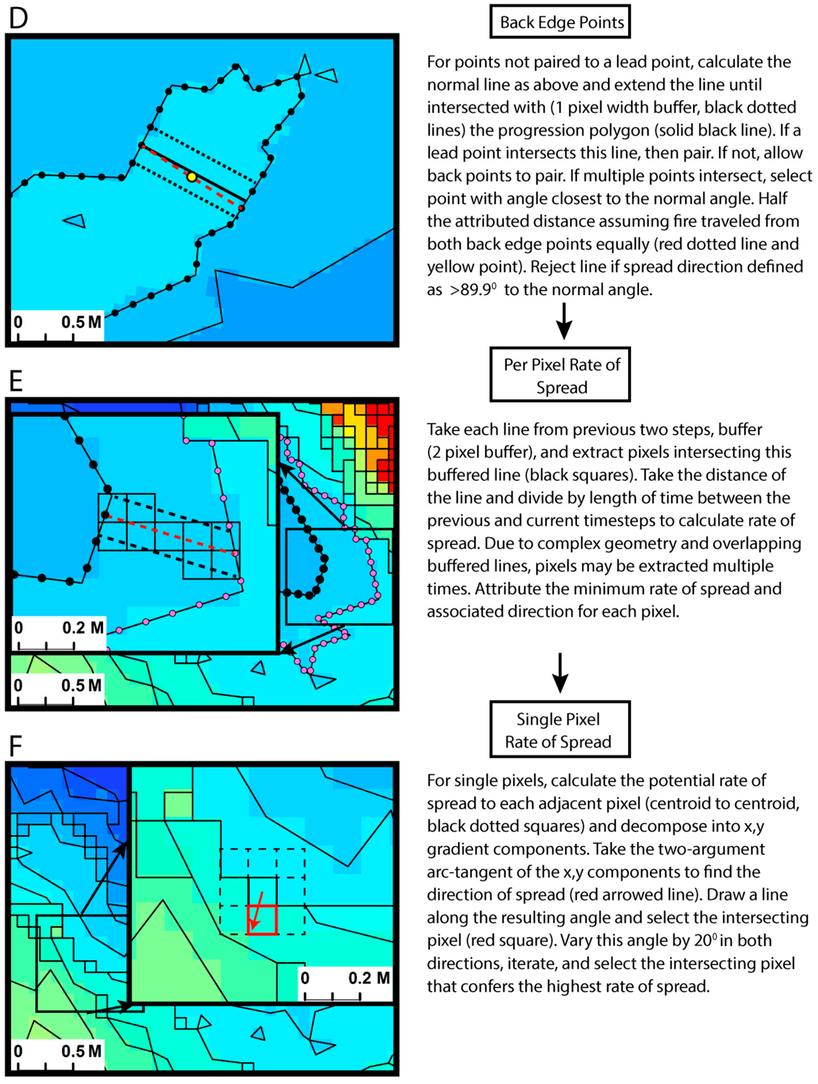
Each focal point was defined as either a lead or back edge point. This was determined by examining the adjacent polygon to the point and assessing whether it burned before or after in time. Leading edge points were connected with lines to back edge points with the logic demonstrated in Figure 1. Back edge points can be connected to multiple lead edge points. This situation represents fire growth in an expanding elliptical pattern, which most spatial fire spread models assume (e.g., FARSITE) [72]. The inverse situation is also possible where the fire closes in from multiple directions resulting in more back edge points than lead edge points. This special situation is highlighted in Figure 1 Box D. Once each point is paired, a straight line connecting the pair was created, which allowed for distance and direction to be determined. The line was buffered with a width of two pixels, and all of the pixels within this area were attributed with the direction and a RoS. The RoS was determined by dividing the length of the line by the length of time between the previous and current images. The buffering of the line leads to some pixels being attributed multiple RoS and directions. In these cases, we attributed the minimum RoS and its associated direction with the assumption that the fire traveled the shortest route.
Another special situation is fire spread of one pixel per timestep, which is not amenable to the vector method above. We borrowed logic from calculation of topographical aspect from digital elevation rasters for these cases. First, we calculated the potential RoS to all the adjacent pixels and decomposed RoS into separate x, y components. The most likely spread direction was taken as the two-argument arc-tangent of the x, y components (‘atan2′ function) [67]. Therefore, this method is built on the assumption that the direction of fastest spread is the most likely. We could not use the same assumption that the shortest route is most likely here, as only one pixel is traversed per timestep. We then placed a line pointed in this resulting direction, found the intersecting pixel, calculated the pixel centroid to centroid distance, determined the length of time to traverse this line, and divided the distance by time to calculate the RoS. The intersection of the spread direction line can clip the corners of pixels that may not be the pixel with the most likely travel path. Thus, we added 20° to the calculated direction line in both directions, iterated the process, and selected the pixel with the highest resulting RoS as the most likely travel path. As pixel resolutions become larger and fire spread slows, individual pixel movement gains in frequency. This method becomes increasingly important for the accurate characterization of fire spread in those situations.
2.9. Analytical Units
The geometrical size and shape of analytical units are important considerations [58]. For RoS, the minimum areal unit of measurement could be considered the point-to-point vector line and intersecting pixels (i.e., Figure 1, Box E). However, considerable overlap occurs between these buffered lines and the point-to-point spacing is arbitrary. Conversely, the progression polygons created from the connected timestep pixels could also be considered a measurement unit. However, these polygons can be quite large and incorporate backing, flanking, and heading fire behavior. We sought to aggregate (or disaggregate depending on the perspective) pixels (or progression polygons) to achieve a medium between these two extremes.
We chose an automated approach using the idea of connected components from graph theory [73,74], hypothesizing that sharp changes in RoS between adjacent pixels delineate the boundaries of relatively independent analytical units. Pixels are considered to be connected when adjacent, within the same timestep, and below a defined change (or tolerance) parameter. The change parameter determines the degree of pixel aggregation. We evaluated a series of values settling on 0.015 m/s for the parameter as reasonable to aggregate to polygons that were relatively homogeneous in terms of the backing, flanking, and heading fire behavior. Tuning this parameter is likely necessary for higher RoS and different degrees of variability though this value was acceptable for the range of RoS observed in this study. We also required a minimum polygon area of 6x6 pixels for progression timesteps with high RoS (polygons sizes > 1 m2) to prevent individual and small groups of pixels from becoming their own units. In these cases, pixels that displayed large deviations in RoS estimates from neighboring pixels were predominantly artifacts of the algorithm (especially areas of complex geometry) and were assumed to not be different units.
3. Results
We evaluated two cold target sizes as GCPs, circular with 12 cm diameter, and square with 40 cm sides, at six altitudes above ground level (AGL) up to 150 m. For polished aluminum with an approximate emissivity coefficient of 0.04, targets must be roughly 1.1 times the size of the pixel to be reliably visible in optical, thermal IR, and NIR imagery assuming line of sight is maintained. At altitudes of 150 m, a ratio of 1.2 is a safer minimum threshold as atmospheric effects become larger. At nadir and lower AGL (<100 m), targets can be half the size of pixels and still have visibility. However with flames surrounding, we observed targets five times larger than a pixel obscured by heat. Eight ground targets distributed throughout the image in our nested square plot layout provided accurate georectification results following image stabilization techniques (RMSE 0.14–0.28 m for Lubrecht and 0.27–0.94 m for Sycan).
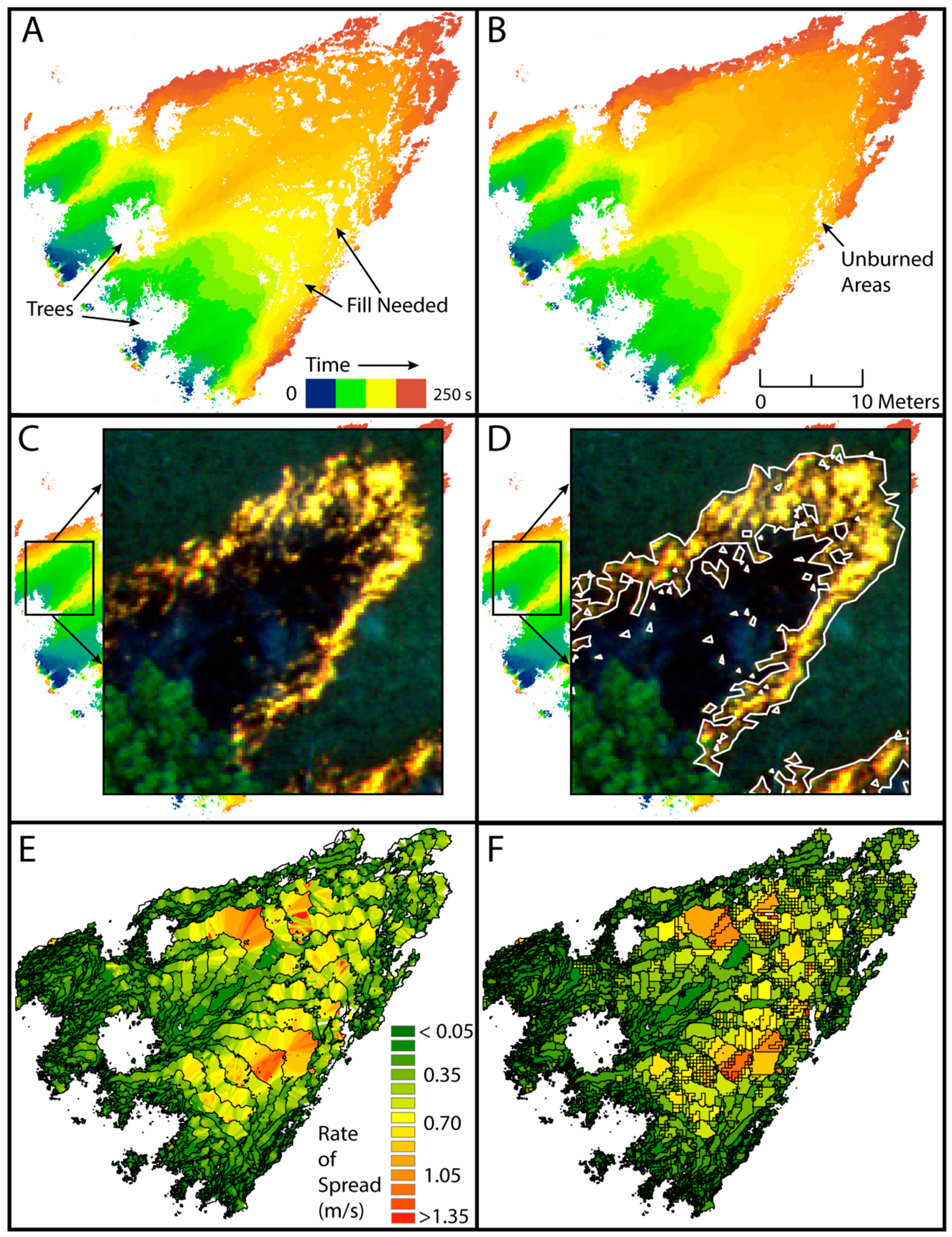
Fire behavior metrics were produced after the images were aligned, calibrated, and georectified. First, fire progression maps from gradient-based threshold techniques were derived (Figure 2, Box A and B). Similar to the results of Valero et al. [37], gradients successfully defined fire movement in thermal imagery. The use of NIR also matched well with optical flame imagery (Figure 2, Box C and D). A 1–3 pixel (8.2–24.6 cm) error of commission was observed at certain portions of the fireline though. This was most conspicuous at the heading portions and along the wind vector (e.g., right side of fireline in Figure 2, Box D). The use of the dual threshold technique filled the burned portions with low residence times and followed the natural flow of the progression (cf. Figure 2, Box A and B), but left unburned areas when visually compared to post-fire imagery (data not shown).
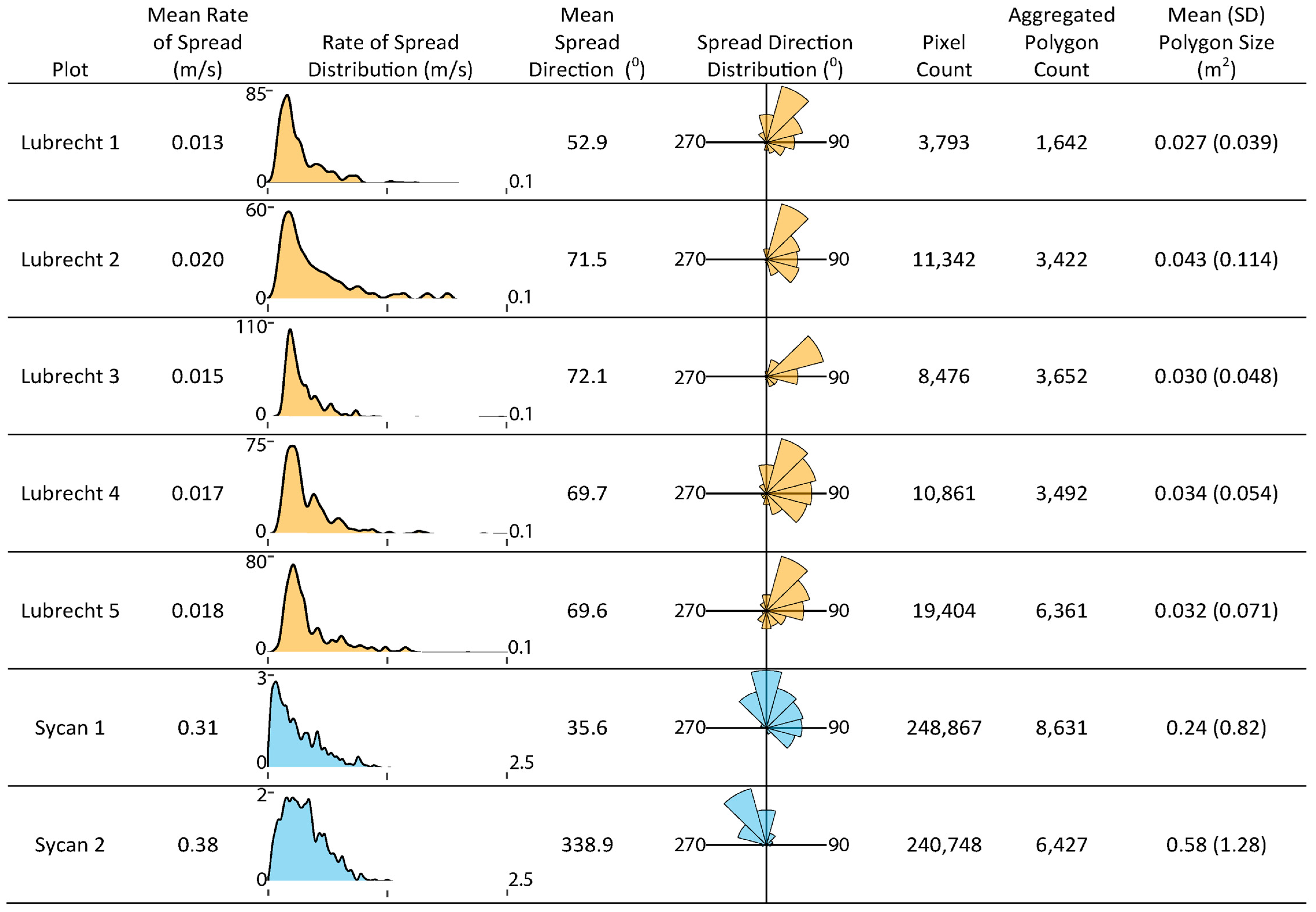
We observed complex fire behavior with multiple heading fires and interacting flanking fires in nearly every plot, despite single strip ignition near each plot. Sycan plot 2 had the most coherent fireline with relatively consistent topography and grass fuels. RoS ranged from 0–2.7 m/s at the two Sycan plots and 0–0.1 m/s for the Lubrecht plots (Figure 3). RoS distributions all had heavy-tailed, positively-skewed distributions with area-weighted mean spread rates of 0.013–0.02 m/s for the Lubrecht plots and 0.305–0.404 m/s for the Sycan plots. Predictably, RoS was highest along the primary vectors of fire travel (heading fire) and lower along the flanks. At Lubrecht, field estimates of RoS were made between the visible targets (GCPs) within each plot. These estimates were significantly correlated with our image-derived measurements (Pearson correlation, n = 12, r = 0.71, p < 0.05). Spread direction followed expectations; though in areas of highly irregular and complex firelines, inconsistencies still emerged despite designs to reduce them.
Spatial aggregation of RoS produced polygon numbers averaging 35.4% of the original pixel count for Lubrecht and 3.1% of the pixels for Sycan (Figure 3), highlighting the large amount of redundant data and the strong influence of spread rate. The areas of inconsistent spread direction due to complex fireline geometry tended to have more polygons as spread rates showed increased variability along sharper gradients within each progression timestep. Aggregated polygons had a mean size of 0.38 m2 for Sycan and 0.033 m2 for Lubrecht. The maximum polygon size was 23.6 m2 for Sycan and 2.8 m2 for Lubrecht.
4. Discussion
Fire metrics based on fire progression estimates are common in the scientific literature though rarely validated [38]. Our estimates of RoS compared well with visual, one-dimension estimates (r = 0.71) and also with mathematical fire model predictions. For example, using observed weather and fuel moisture parameters at Lubrecht and the timber litter and understory fuel model, Rothermel’s [75] fire spread equation predicts heading fire spread rates of 0.0045–0.060 m/s, which compares favorably to the 0–0.1 m/s range observed.
Spread direction followed general expectations with heading fire moving in the observed primary spread direction. However, our results show an interesting pattern related to fireline coherency and the relative amounts of flanking and heading fire. As mentioned, Sycan plot 2 had the most coherent fireline and the direction histogram shows the majority of spread in the same direction. In contrast, the majority of Lubrecht plot 5 experienced spread directions that were nearly orthogonal (mean 69.6° from North) to the direction of the heading fires (c. 135°). All of the Lubrecht plots show this spread direction distribution to varying degrees with plot 5 as the most prominent. The discontinuous surface fuels are likely the primary cause of this behavior. The burn occurred in a previously thinned area having numerous stumps, abundant 100-to 1000-hr fuel class (2.54–20.32 cm diameter) woody debris, and skid trails left from mechanized equipment. The heading fires followed paths with sufficient fine fuels and then flanked and backed into areas where the barriers (e.g., larger fuels) had stopped the initial flame front. The associated changes in fire behavior have implications for fire effects [18].
Multiple heading fires also led to multiple firelines interacting, and the design of the algorithm properly identified and estimated RoS in these situations with one significant caveat. Some of these interaction zones, for example, the center of Sycan plot 1 (Figure 2, Box A), had lower RoS than anticipated. The preceding polygons showed a rise in RoS as the two flanking fires interacted, but RoS then decreased at the converging polygon. This artifact arose as a result of the temporal resolution of data capture being considerably slower than the RoS, and from the assumption that the fire spread at an equal rate from each fire line. Although between-image fire behavior can be inferred, assumptions are inherently necessary. For example, total radiant energy or intensity metrics could be used to infer higher than observed RoS or to determine the predominant direction of spread rather than assuming equal rates from both directions.
The area traversed by fire between consecutive images causes a lack of data as fire behavior in the intervening time period is unknown. As RoS is a derivative of fire progression and fire progression is a derivative of the time-series imagery, it is possible and tempting to attribute each pixel from the progression or time-series layers with a RoS value. However, our analysis shows that the majority of these pixels are not measurement units nor statistically independent. The statistical consequences are inflated or introduced spatial autocorrelation and pseudo-replication [56]. The approach proposed here does risk a loss of relevant data if the change parameter is too high in value or RoS is spatially homogenous. This could lead to large analytical units. For example, long, linear fire fronts with consistent RoS could be aggregated to one or a few analytical units within a timestep (we emphasize that the units here were aggregated within individual timesteps and not beyond). This issue could also be exacerbated by coarse temporal resolution imagery. We focused on creating robust analytical units for subsequent pattern-process relationships. From this perspective, consistent RoS implies either consistent underlying patterns or little influence of pattern on fire processes, either case would be discoverable with analysis using larger analytical units. The analytical unit derivation strategy may need to be reconsidered for other analytical objectives. A potential research direction would be to follow the general approach of Openshaw and Taylor [57] and systematically vary analytical units and assess the effect on resulting spatial relationships. See Gelfand [76] for an in-depth review of existing literature and strategies for the change of the support problem.
We hypothesized that this issue could be leveraged to help inform other data sampling methods. The analytical unit size is dependent on the interaction of RoS and the temporal and spatial resolution of the time-series imagery. Thus, with RoS predictions and known camera parameters, estimates of the analytical unit sizes are possible pre-fire. This information could provide guidance for field sampling protocols, especially plot sizes, and unit sizes for other remotely-sensed data. For example, UAS platforms have enabled increasingly fine-grained pre- and post-fire 3-D vegetation data [50]. The data density from these photogrammetrically-derived point clouds can be hundreds to thousands of points per square meter, and thus the level of spatial aggregation that minimizes the loss of pertinent information while removing redundancy is becoming a research priority. The analytical units of fire behavior are likely to be larger and of variable size when compared to this vegetation data as we show in this study. Ultimately, these datasets will need to be transformed and aligned if characterization of fire behavior and fire environment interaction is the objective. With additional research, derivation of a generalized relationship between RoS and camera parameters and the resulting analytical unit sizes can be useful for the production and analysis of comprehensive datasets.
Lessons Learned
UAS promise relatively cheap and low risk aviation platforms that provide new remote sensing capabilities to a variety of users. In the course of our experiences over the last few years, we evaluated many off-the-shelf and custom-built UAS. These experiences enable us to provide some suggestions for fire researchers interested in employing UAS in their work. First, we advise to not focus on flight capabilities alone. Flight time, speed, maneuverability, and payload are important, but sensor hardware integration, quality of software, spare parts availability, and ease of repair are equally, if not more, consequential to successful data collection. Custom or boutique UAS often promise improved or specific performance capabilities but frequently lack available spare parts and are often beset with hardware and software issues. Better flight performance and larger payloads also require larger UAS, which are cumbersome to transport, an important consideration in dynamic and time sensitive field settings. We place a premium on small, cheap, reliable systems, which often means working with consumer-grade technology provided by established companies.
We found that software issues were common in nearly all of the systems that we tested to varying degrees. At one point, three different software applications, two being third-party, were required to execute pre- and during-fire data collection within a single mission. How software interacts is unknown after any updates to the myriad of systems, and mission workflows must then be retested in entirety. Automatic software updates are often applied without notification and would frequently change system behavior. Considering the resources needed to plan data collection, coordinate with fire operations, meet acceptable burn conditions (weather, fuel moisture, time of season, etc.), and have needed resources available, the chance of hardware or software failure must be minimized. Often, this level of coordination and timing only comes together for a few days out of one or more years. Thus, the importance of a dependable UAS cannot be understated with emphasis on the system (e.g., platform, sensors, software, planning).
During our prescribed burn campaigns, the UAS experienced extremes ranging from heat from fire, freezing temperatures, heavy smoke and dust, high winds, attacks from territorial birds, and nearly all forms of precipitation. Given the likelihood of such situations in field conditions, we recommend building redundancy, such as having duplicate UAS available with exactly replicated hardware and software configurations. We also recommend platforms with weather resistance. The sensors described in this study cost more than the UAS and, if cost is an issue, we recommend having duplicate platforms over sensors as the probability of platform malfunction is usually greater.
For the use of UAS in prescribed fire experiments, plot locations must strike a balance of achieving desired experimental results while also operating within the context of prescribed burn operations. Field-based fire research generally needs to be opportunistic and in harmony with burn objectives. The majority of prescribed burn units in the US are fired in one day, and coordination and timing with the operations team throughout the day is of utmost importance. Unless multiple UAS teams are available, each research plot must be positioned in order to allow enough time to collect data at a plot, disassemble, and then reassemble at a new launch location before burn operations are ready to fire the next plot. Alternatively, it may be logical to fly multiple plots from one location. This strategy can significantly reduce the flight time for data collection though. We chose to travel the fire perimeter to locations near each plot where the UAS was viewable by the pilot. The pre-planning for these logistics can be complex as operational firing plans change based on weather conditions, particularly wind directions. Plot layouts designed for a single spread direction due to fuel or topography arrangement often do not follow expectations if winds shift. For example, a plot could be burned at either the start or end of burn operations, depending on wind directions, with large subsequent changes in fire behavior. Successful implementation of UAS in prescribed burn experiments requires flexibility to weather conditions while also ensuring that research efforts do not impede firing or holding operations.
In our study, plots were selected and fired to reach steady state fire spread and produce a coherent fireline before reaching the plot edge. In practice, heterogeneous fuels and shifting winds meant ignition at variable distances and directions in relation to the plots, including through the plot in one instance (Sycan plot 1). Timing UAS takeoff in conjunction with ignition in these conditions proved to be difficult, requiring consideration of different tradeoffs. If takeoff is too early, then battery life will be expended without gathering useful data; conversely, if takeoff is too late, fire may enter the plot before data collection begins. The time to prepare a UAS for launch is also variable depending on multiple devices booting, cameras initializing, and achieving a GPS fix. A vantage point where the UAS pilot can view burn operations is optimal for timing, but often not likely due to fire, smoke, and tree interference. Prompt, succinct, and informative radio communication is vital, which usually necessitates a radio liaison communicating between pilots, visual observers, operational personnel, and the actual plot ignitor. Ideally, personnel with the necessary fire qualifications and sufficient familiarity with the research and plot design are inserted into the operational command structure to facilitate the necessary coordination.
5. Conclusions
UAS can give an unprecedented perspective for data collection in active fire environments at favorable spatial and temporal scales if the software, hardware, and fire operations conflicts are resolved or minimized. Robust data collection workflows must constantly evolve while still maintaining coherent scientific rigor due to the rapid and ongoing development of UAS and sensor technology.
With the new perspective provided by UAS, we are able to image complex fire behavior that necessitated updated algorithms capable of characterizing such behavior. Fire behavior is missed between sample intervals requiring dynamic analytical unit sizes. The nature of this relationship is largely dependent on RoS and the temporal and spatial resolution of the sensor. Characterizing this relationship in a generalized fashion is likely possible with additional research and could potentially inform other pre- and post-fire sampling methods for the ultimate goal of comprehensive datasets of the fire environment.
The collection of such comprehensive datasets that characterize fuels, fire behavior, weather, and, if possible, emissions and fire effects, are essential for evaluation of models and for cross-disciplinary knowledge gains in the broader field of wildland fire science. Research projects that attempt to create such datasets are substantial endeavors. UAS could be a unifying remote sensing platform that collects such datasets in a safe and relatively inexpensive manner. Ultimately, UAS provide complementary capabilities that enhance our ability to understand how fires burn.
Author Contributions
Conceptualization, C.M., C.S., R.P., and L.Q.; Methodology, C.M., C.S., M.C., V.H., R.P., K.S., L.Q., T.W.; Formal analysis, C.M.; Resources, C.S., R.P., K.S., and L.Q.; Writing—original draft preparation, C.M. and C.S.; Writing—review and editing, M.C., V.H., R.P., K.S., L.Q., and T.W.; Funding acquisition, C.S., R.P., and L.Q.
Funding
This research was supported by funds from the Western Wildlands Environmental Threat Assessment Center (WWETAC) through a modification to Research Joint Venture Agreement 15-JV-11221637-122, by the state of Montana Research and Development Initiative, and by the University of Montana’s National Center for Landscape Fire Analysis.
Acknowledgments
We acknowledge The Oregon Nature Conservancy, Fremont-Winema National Forest, and Lubrecht Experimental Forest for personnel, resources, and additional assistance for the prescribed burns that were instrumental to this research. Two anonymous reviewers significantly contributed to the improvement of this article.
Conflicts of Interest
The authors declare no conflict of interest.
References
- Stocks, B.J.; Alexander, M.E.; Lanoville, R.A. Overview of the international crown fire modelling experiment (ICFME). Can. J. For. Res. 2004, 34, 1543–1547. [Google Scholar] [CrossRef]
- Clements, C.B.; Zhong, S.; Goodrick, S.; Li, J.; Potter, B.E.; Bian, X.; Heilman, W.E.; Charney, J.J.; Perna, R.; Jang, M.; et al. The dynamics of wildland grass fires: FireFlux—A field validation experiment. Bull. Am. Meteor. Soc. 2007, 88, 1369–1382. [Google Scholar] [CrossRef]
- Kremens, R.L.; Smith, A.M.S.; Dickinson, M.B. Fire metrology: Current and future direction in physics–based measuremens. Fire Ecology 2010, 6, 13–35. [Google Scholar] [CrossRef]
- Ottmar, R.D.; Hiers, J.K.; Butler, B.W.; Clements, C.B.; Dickinson, M.B.; Hudak, A.T.; O’Brien, J.J.; Potter, B.E.; Rowell, E.M.; Strand, T.M.; et al. Measurements, datasets and preliminary results from the RxCADRE project–2008, 2011 and 2012. Int. J. Wildl. Fire 2016, 25, 1–9. [Google Scholar] [CrossRef]
- Finney, M.A.; Cohen, J.D.; Forthofer, J.M.; McAllister, S.S.; Gollner, M.J.; Gorham, D.J.; Saito, K.; Akafuah, N.K.; Adam, B.A.; English, J.D. Role of buoyant flame dynamics in wildfire spread. Proc. Nat. Acad. Sci. USA 2015, 112, 9833–9838. [Google Scholar] [CrossRef] [PubMed] [Green Version]
- Finney, M.A.; Cohen, J.D.; McAllister, S.S.; Jolly, W.M. On the need for a theory of wildland fire spread. Int. J. Wildl. Fire 2013, 22, 25–36. [Google Scholar] [CrossRef] [Green Version]
- Sauvagnargues–Lesage, S.; Dusserre, G.; Robert, F.; Dray, G.; Pearson, D.W. Experimental validation in Mediterranean shrub fuels of seven wildland fire rate of spread models. Int. J. Wildl. Fire 2001, 10, 15–22. [Google Scholar] [CrossRef]
- Mell, W.; Jenkins, M.A.; Gould, J.; Cheney, P. A physics–based approach to modelling grassland fires. Int. J. Wildl. Fire 2007, 16, 1–22. [Google Scholar] [CrossRef]
- Achtemeier, G.L. Field validation of a free–agent cellular automata model of fire spread with fire–atmosphere coupling. Int. J. Wildl. Fire 2012, 22, 148–156. [Google Scholar] [CrossRef]
- Alexander, M.E.; Cruz, M.G. Are the applications of wildland fire behavior models getting ahead of their evaluation again? Environ. Model. Softw. 2013, 41, 65–71. [Google Scholar] [CrossRef]
- Buma, B.; Wessman, C.A. Disturbance interactions can impact resilience mechanisms of forests. Ecosphere 2011, 2, 1–13. [Google Scholar] [CrossRef]
- Jenkins, M.J.; Runyon, J.B.; Fettig, C.J.; Page, W.G.; Bentz, B.J. Interactions among the mountain pine beetle, fires, and fuels. For. Sci. 2014, 60, 489–501. [Google Scholar] [CrossRef]
- Finney, M.A.; McHugh, C.W.; Grenfell, I.C. Stand– and landscape–level effects of prescribed burning on two Arizona wildfires. Can. J. For. Res. 2005, 35, 1714–1722. [Google Scholar] [CrossRef]
- Cochrane, M.A.; Moran, C.J.; Wimberly, M.C.; Baer, A.D.; Finney, M.A.; Beckendorf, K.L.; Eidenshink, J.; Zhu, Z. Estimation of wildfire size and risk changes due to fuels treatments. Int. J. Wildl. Fire 2011, 21, 357–367. [Google Scholar] [CrossRef]
- Ziegler, J.P.; Hoffman, C.; Battaglia, M.; Mell, W. Spatially explicit measurements of forest structure and fire behavior following restoration treatments in dry forests. For. Ecol. Manag. 2016, 286, 1–12. [Google Scholar] [CrossRef]
- Thaxton, J.M.; Platt, W.J. Small–scale fuel variation alters fire intensity and shrub abundance in a pine savanna. Ecology 2006, 87, 1331–1337. [Google Scholar] [CrossRef]
- Loudermilk, E.L.; O’Brien, J.J.; Mitchell, R.J.; Cropper, W.P.; Hiers, J.K.; Grunwald, S.; Grego, J.; Fernandez–Diaz, J.C. Linking complex forest fuel structure and fire behavior at fine scales. Int. J. Wildl. Fire 2012, 21, 882–893. [Google Scholar] [CrossRef]
- O’Brien, J.J.; Loudermilk, E.L.; Hiers, J.K.; Pokswinski, S.M.; Hornsby, B.; Hudak, A.T.; Strother, D.; Rowell, E.; Bright, B.C. Canopy–derived fuels drive patterns of in–fire energy release and understory plant mortality in a longleaf pine (Pinus palustris) sandhill in northwest Florida, USA. Can. J. Remote Sens. 2016, 42, 489–500. [Google Scholar] [CrossRef]
- Johannsson, N. Numerical Experiments a Research Method in Fire Science; Lund University: Lund, Sweden, 2013. [Google Scholar]
- Lentile, L.B.; Holden, Z.A.; Smith, A.M.S.; Falkowski, M.J.; Hudak, A.T.; Morgan, P.; Lewis, S.A.; Gessler, P.E.; Benson, N.C. Remote sensing techniques to assess active fire characteristics and post–fire effects. Int. J. Wildl. Fire 2006, 15, 319–345. [Google Scholar] [CrossRef]
- Wooster, M.J.; Roberts, G.; Perry, G.L.W.; Kaufman, Y.J. Retrieval of biomass combustion rates and totals from fire radiative power observations: FRP derivation and calibration relationships between biomass consumption and fire radiative energy release. J. Geophys. Res. Atmos. 2005, 110. [Google Scholar] [CrossRef]
- Freeborn, P.H.; Wooster, M.J.; Hao, W.M.; Ryan, C.A.; Nordgren, B.L.; Baker, S.P.; Ichoku, C. Relationships between energy release, fuel mass loss, and trace gas and aerosol emission during laboratory biomass fires. J. Geophys. Res. Atmos. 2008, 113. [Google Scholar] [CrossRef]
- Dupuy, J.-L.; Maréchal, J.; Portier, D.; Valette, J.-C. The effects of slope and fuel bed width on laboratory fire behavior. Int. J. Wildl. Fire 2011, 20, 272–288. [Google Scholar] [CrossRef]
- May, N.; Ellicott, E.; Gollner, M. An examination of fuel moisture, energy release, and emissions during laboratory burning of live wildland fuels. Int. J. Wildl. Fire 2019, 28, 187–197. [Google Scholar] [CrossRef]
- Wooster, M.J. Small–scale experimental testing of fire radiative energy for quantifying mass combusted in natural vegetation fires. Geophys. Res. Lett. 2002, 29, 1–23. [Google Scholar] [CrossRef]
- Frankman, D.; Webb, B.W.; Butler, B.W.; Jimenez, D.; Forthofer, J.M.; Sopko, P.; Shannon, K.S.; Hiers, J.K.; Ottmar, R.D. Measurements of convective and radiative heating in wildland fires. Int. J. Wildl. Fire 2012, 22, 157–167. [Google Scholar] [CrossRef]
- Dickinson, M.B.; Hudak, A.T.; Zajkowski, T.; Loudermilk, E.L.; Schroeder, W.; Ellison, L.; Kremens, R.L.; Holley, W.; Martinez, O.; Paxton, A.; et al. Measuring radiant emissions from entire prescribed fires with ground, airborne and satellite sensors-RxCADRE 2012. Int. J. Wildl. Fire 2016, 25, 48–61. [Google Scholar] [CrossRef]
- Ichoku, C.; Giglio, L.; Wooster, M.J.; Remer, L.A. Global characterization of biomass–burning patterns using satellite measurements of fire radiative energy. Remote Sens. Environ. 2008, 112, 2950–2962. [Google Scholar] [CrossRef]
- Roberts, G.; Wooster, M.J.; Lagoudakis, E. Annual and diurnal African biomass burning temporal dynamics. Biogeosciences 2009, 6, 849–866. [Google Scholar] [CrossRef]
- Vermote, E.; Ellicot, E.; Dubovik, O.; Lapyonok, T.; Chin, M.; Giglio, L.; Roberts, G.J. An approach to estimate global biomass burning emissions of organic and black carbon from MODIS fire radiative power. J. Geophys. Res. Atmos. 2009, 114, D18. [Google Scholar] [CrossRef]
- Sparks, A.M.; Kolden, C.A.; Smith, A.M.S.; Boschetti, L.; Johnson, D.M.; Cochrane, M.A. Fire intensity impacts on post–fire temperate coniferous forest net primary productivity. Biogeosciences 2018, 15, 1173–1183. [Google Scholar] [CrossRef]
- Boschetti, L.; Roy, D.P. Strategies for the fusion of satellite fire radiative power with burned area data for fire radiative energy derivation. J. Geophys. Res. Atmos. 2009, 114. [Google Scholar] [CrossRef] [Green Version]
- Kumar, S.S.; Roy, D.P.; Boschetti, L.; Kremens, R.L. Exploiting the power law distribution properties of satellite fire radiative power retrievals: A method to estimate fire radiative energy and biomass burned from sparse satellite observations. J. Geophys. Res. Atmos. 2011, 116. [Google Scholar] [CrossRef] [Green Version]
- Freeborn, P.H.; Wooster, M.J.; Roy, D.P.; Cochrane, M.A. Quantification of MODIS fire radiative power (FRP) measurement uncertainty for use in satellite–based active fire characterization and biomass burning estimation. Geophys. Res. Lett. 2014, 41, 1988–1994. [Google Scholar] [CrossRef]
- Hudak, A.T.; Freeborn, P.H.; Lewis, S.A.; Hood, S.M.; Smith, H.Y.; Hardy, C.C.; Kremens, R.L.; Butler, B.W.; Teske, C.; Tissell, R.G.; et al. The Cooney Ridge Fire Experiment: An Early Operation to Relate Pre–, Active, and Post–Fire Field and Remotely Sensed Measurements. Fire 2018, 1, 10. [Google Scholar] [CrossRef]
- Paugam, R.; Wooster, M.J.; Roberts, G. Use of handheld thermal imager data for airborne mapping of fire radiative power and energy and flame front rate of spread. IEEE Tran. Geosci. Remote Sens. 2013, 51, 3385–3399. [Google Scholar] [CrossRef]
- Valero, M.M.; Rios, O.; Pastor, E.; Planas, E. Automated location of active fire perimeters in aerial infrared imaging using unsupervised edge detectors. Int. J. Wildl. Fire 2018, 27, 241–256. [Google Scholar] [CrossRef]
- Johnston, J.M.; Wheatley, M.J.; Wooster, M.J.; Paugam, R.; Davies, G.M.; DeBoer, K.A. Flame–front rate of spread estimates for moderate scale experimental fires are strongly influenced by measurement approach. Fire 2018, 1, 16. [Google Scholar] [CrossRef]
- Stow, D.; Riggan, P.; Schag, G.; Brewer, W.; Tissell, R.; Coen, J.; Storey, E. Assessing uncertainty and demonstrating potential for estimating fire rate of spread at landscape scales based on time sequential airborne thermal infrared imaging. Int. J. Remote Sens. 2019, 40, 4876–4897. [Google Scholar] [CrossRef]
- Johnston, J.M.; Wooster, M.J.; Paugam, R.; Wang, X.; Lynham, T.J.; Johnston, L.M. Direct estimation of Byram’s fire intensity from infrared remote sensing imagery. Int. J. Wildl. Fire 2017, 26, 668–684. [Google Scholar] [CrossRef]
- Watts, A.C.; Ambrosia, V.G.; Hinkley, E.A. Unmanned aircraft systems in remote sensing and scientific research: Classification and considerations of use. Remote Sens. 2012, 4, 1671–1692. [Google Scholar] [CrossRef]
- Yuan, C.; Zhang, Y.; Liu, Z. A survey on technologies for automatic forest fire monitoring, detection, and fighting using unmanned aerial vehicles and remote sensing techniques. Can. J. Remote Sens. 2015, 45, 783–792. [Google Scholar] [CrossRef]
- Pérez, Y.; Pastor, E.; Planas, E.; Plucinksi, M.; Gould, J. Computing forest fires aerial suppression effectiveness by IR monitoring. Fire Saf. J. 2011, 46, 2–8. [Google Scholar] [CrossRef]
- McRae, D.J.; Jin, J.-Z.; Conard, S.G.; Sukhinin, A.I.; Ivanova, G.A.; Blake, T.W. Infrared characterization of fine–scale variability in behavior of boreal forest fires. Can. J. For. Res. 2005, 35, 2194–2206. [Google Scholar] [CrossRef]
- Mueller, E.V.; Skowronski, N.; Clark, K.; Gallagher, M.; Kremens, R.L.; Thomas, J.C.; Houssami, M.E.; Filkov, A.; Hadden, R.M.; Mell, W.; et al. Utilization of remote sensing techniques for the quantification of fire behavior in two pine stands. Fire Safety, J. 2017, 91, 845–854. [Google Scholar] [CrossRef] [Green Version]
- Loudermilk, E.L.; Achtemeier, G.L.; O’Brien, J.J.; Hiers, J.K.; Hornsby, B.S. High–resolution observations of combustion in heterogeneous surface fuels. Int. J. Wildl. Fire 2014, 23, 1016–1026. [Google Scholar] [CrossRef]
- Hardin, P.J.; Lulla, V.; Jensen, R.R.; Jensen, J.R. Small unmanned aerial systems (sUAS) for environmental remote sensing: Challenges and opportunities revisited. GISCI Remote Sens. 2019, 56, 309–322. [Google Scholar] [CrossRef]
- Twidwell, D.; Allen, C.R.; Detweiler, C.; Higgins, J.; Laney, C.; Elbaum, S. Smokey comes of age: Unmanned aerial systems for fire management. Front. Ecol. Environ. 2016, 14, 333–339. [Google Scholar] [CrossRef]
- Bright, B.C.; Loudermilk, E.L.; Pokswinksi, S.M.; Hudak, A.T.; O’Brien, J.J. Introducing close–range photogrammetry for characterizing forest understory plant diversity and surface fuel structure at fine scales. Can. J. Remote Sens. 2016, 42, 460–472. [Google Scholar] [CrossRef]
- Shin, P.; Sankey, T.; Moore, M.M.; Thode, A.E. Evaluating unmanned aerial vehicle images for estimating forest canopy fuels in a ponderosa pine stand. Remote Sens. 2018, 10, 1266. [Google Scholar] [CrossRef]
- Samiappan, S.; Hathcock, L.; Turnage, G.; McCraine, C.; Pitchford, J.; Moorhead, R. Remote sensing of wildfire using small unmanned aerial system: Post–fire mapping, vegetation recovery and damage analysis in Grand Bay, Mississippi/Alabama, USA. Drones 2019, 3, 43. [Google Scholar] [CrossRef]
- Loudermilk, E.L.; Hiers, J.K.; O’Brien, J.J.; Mitchell, R.J.; Singhania, A.; Fernandez, J.C.; Cropper, W.P. Jr.; Slatton, K.C. Ground–based LIDAR: A novel approach to quantify fine–scale fuelbed characteristics. Int. J. Wildl. Fire 2009, 18, 676–685. [Google Scholar] [CrossRef]
- Lefsky, M.A.; Cohen, W.B.; Parker, G.G.; Harding, D.J. Lidar remote sensing for ecosystem studies. Bioscience 2002, 52, 19–30. [Google Scholar] [CrossRef]
- Hiers, J.K.; O’Brien, J.J.; Mitchell, R.J.; Grego, J.M.; Loudermilk, E.L. The wildland fuel cell concept: An approach to characterize fine–scale variation in fuels and fire in frequently burned longleaf pine forests. Int. J. Wildl. Fire 2009, 18, 315–325. [Google Scholar] [CrossRef]
- Anderson, W.R.; Catchpole, E.A.; Butler, B.W. Convective heat transfer in fire spread through fine fuel beds. Int. J. Wildl. Fire 2010, 19, 284–298. [Google Scholar] [CrossRef]
- Bataineh, A.L.; Oswald, B.P.; Bataineh, M.; Unger, D.; Hung, I.-K.; Scognamillo, D. Spatial autocorrelation and pseudo replication in fire ecology. Fire Ecol. 2006, 2, 107–118. [Google Scholar] [CrossRef]
- Openshaw, S.; Taylor, P. A Million or so Correlation Coefficients: Three Experiments on the Modifiable Areal Unit Problem. In Statistical Applications in the Spatial Sciences; Wrigley, N., Ed.; Pion: London, UK, 1979; Volume 1, pp. 127–144. [Google Scholar]
- Gotway, C.A.; Young, L.J. Combining incompatible spatial data. J. Am. Stat. Assoc. 2002, 97, 632–648. [Google Scholar] [CrossRef]
- Valero, M.M.; Jimenez, D.; Butler, B.W.; Mata, C.; Rios, O.; Pastor, E.; Planas, E. On the use of compact thermal cameras for quantitative wildfire monitoring. In Proceedings of the 8th International Conference on Forest Fire Research Proceedings, Coimbra, Portugal, 9–16 November 2018. [Google Scholar]
- Johnston, J.M.; Wooster, M.J.; Lynham, T.J. Experimental confirmation of the MWIR and LWIR grey body assumption for vegetation fire flame emissivity. Int. J. Wildl. Fire 2014, 23, 463–479. [Google Scholar] [CrossRef]
- Micasense Image Processing. Available online: https://github.com/micasense/imageprocessing (accessed on 1 December 2018).
- O’Brien, J.J.; Loudermilk, E.L.; Hornsby, B.; Hudak, A.T.; Bright, B.C.; Dickinson, M.B.; Hiers, J.K.; Teske, C.; Ottmar, R.D. High–resolution infrared thermography for capturing wildland fire behavior—RxCADRE 2012. Int. J. Wildl. Fire 2016, 25, 62–75. [Google Scholar] [CrossRef]
- Ononye, A.; Vodacek, A.; Saber, E. Automated extraction of fire line parameters from multispectral infrared images. Remote Sens. Environ. 2007, 108, 179–188. [Google Scholar] [CrossRef] [Green Version]
- Canny, J. A Computational Approach to Edge Detection. In Readings in Computer Vision; Fischler, M.A., Firschein, O., Eds.; Morgan Kaufmann: Burlington, USA, 1987; pp. 184–203. [Google Scholar]
- Lloyd, S.P. Least squares quantization in PCM. IEEE Trans. Inf. Theory 1982, 28, 129–137. [Google Scholar] [CrossRef]
- Boschetti, L.; Flasse, S.P.; Brivio, P.A. Analysis of the conflict between omission and comission in low spatial resolution dichotomic thematic products: The Pareto Boundary. Remote Sens. Environ. 2004, 91, 280–292. [Google Scholar] [CrossRef]
- R Core Team. R: A Language and Environment for Statistical Computing; R Foundation for Statistical Computing: Vienna, Austria, 2010. Available online: http://www.R–project.org/ (accessed on 1 January 2018).
- Hijmans, R.J. Raster: Geographic Data Analysis and Modeling. 2018, R Package Version 2.8-4. Available online: https://cran.r–project.org/package=raster (accessed on 15 December 2018).
- Pebesma, E.J.; Bivand, R.S. Classes and Methods for Spatial Data in R. 2005, R News 5(2). Available online: https://cran.r–project.org/doc/Rnews (accessed on 15 December 2018).
- Bivand, R.S.; Rundel, C. Rgeos: Interface to Geometry Engine—Open Source (‘GEOS’). 2018, R Package Version 0.4-2. Available online: https://cran.r–project.org/packages=rgeos (accessed on 15 December 2018).
- Agostinelli, C.; Lund, U. Circular: Circular Statistics. 2017, R Package Version 0.4-93. Available online: https://r–forge.r–project.org/projects/circular (accessed on 15 December 2018).
- Finney, M.A. FARSITE: Fire Area Simulator–Model Development and Evaluation; Res. Pap. RMRS-RP-4; Department of Agriculture, Forest Service, Rocky Mountain Research Station: Ogden, UT, USA, 1998; 47p.
- Tarjan, R. Depth–first search and linear graph algorithms. SIAM J. Computing 1972, 1, 146–160. [Google Scholar] [CrossRef]
- Barthelme, S. Imager: Image Processing Library Based on ‘CImg’. 2018, R Package Version 0.41.1. Available online: https:// cran.r–project.org/package=imager (accessed on 15 December 2018).
- Rothermel, R.C. A Mathematical Model for Predicting Fire Spread in Wildland Fuels; Res. Pap. INT–115; Department of Agriculture, Forest Service, Rocky Mountain Research Station: Ogden, UT, USA, 1972; 40p.
- Gelfand, A.E. Misaligned spatial data: The change of support problem. In Handbook Spatial Statistics, 1st ed.; Gelfand, A.E., Diggle, P.J., Fuentes, M., Guttorp, P., Eds.; CRC Press: Boca Raton, FL, USA, 2010; pp. 517–539. [Google Scholar]
Figure 1.
Description of the rate of spread algorithm including situations requiring additional consideration when experiencing complex fire behavior (Box D and F). Illustrated examples taken from Lubrecht plot 5.
Figure 1.
Description of the rate of spread algorithm including situations requiring additional consideration when experiencing complex fire behavior (Box D and F). Illustrated examples taken from Lubrecht plot 5.


Figure 2.
UAS data and derived metrics from Plot 1, Sycan Marsh, OR. (A) Fire progression with tree occlusion and additional missing data due to low flame residence time. (B) Data gaps filled using dual-threshold flaming combustion definition. (C) Optical (RGB) imagery from Micasense RedEdge camera highlighting one of the multiple heading fires within the plot. (D) Outline (white lines) of flaming combustion as defined by the method described in Section 2.6. (E) Calculated rate of spread delineated by image timesteps (black lines). (F) Automated aggregation of polygons to create analytical units.

Figure 3.
Fire spread rate and direction from Lubrecht, MT and Sycan Marsh, OR plots. Pixel count, aggregated polygon count, and mean polygon size shown to highlight the large amount of redundant data and the loss of perceived sample size (pixels vs. aggregated polygons) after removal. All y-axes are scaled independently for ease of viewing and represent probability density functions.


Table 1.
Sensor and data collection information for the two prescribed burns (Lubrecht and Sycan) in this study.
Table 1.
Sensor and data collection information for the two prescribed burns (Lubrecht and Sycan) in this study.
| Sensor | Spectral Band for Fire Behavior | Radiometric Temperature Range 1 | Array Size | Plot | Altitude Above Ground | Ground Sample Distance | Temporal Resolution | Time Series Length |
|---|---|---|---|---|---|---|---|---|
| (Focal Length) | (µm) | (°C) | (Pixels) | Name | (m) | (cm) | (Hz) | (s) |
| FLIR XT (9 mm) 2 | 7.5–13.5 | 100–1100 | 640 × 512 | Lubrecht 1 | 19 | 3.59 | 0.13 | 725 |
| FLIR XT (9 mm) 2 | 7.5–13.5 | 100–1100 | 640 × 512 | Lubrecht 2 | 20 | 3.78 | 0.13 | 1216 |
| FLIR XT (9 mm) 2 | 7.5–13.5 | 100–1100 | 640 × 512 | Lubrecht 3 | 20 | 3.78 | 0.13 | 1449 |
| FLIR XT (9 mm) 2 | 7.5–13.5 | 100–1100 | 640 × 512 | Lubrecht 4 | 18.5 | 3.49 | 0.13 | 1014 |
| FLIR XT (9 mm) 2 | 7.5–13.5 | 100–1100 | 640 × 512 | Lubrecht 5 | 18 | 3.41 | 0.12 | 928 |
| FLIR XT (9 mm) | 7.5–13.5 | 100–190 3 | 640 × 512 | Sycan 1 | 120 | 22.7 | 0.2 | 250 |
| MicaSense RedEdge (5.4 mm) | 0.82–0.86 | 650–1150 4 | 1280 × 960 | Sycan 1 | 120 | 8.2 | 0.2 | 250 |
| MicaSense RedEdge (5.4 mm) | 0.82–0.86 | 650–1150 4 | 1280 × 960 | Sycan 2 | 180 | 12.5 | 0.2 | 240 |
1 Tested on a Mikron M300 blackbody calibration source with a 100–1150 °C temperature range; 2 Higher temperature range achieved using a custom neutral-density filter; 3 High gain setting without neutral-density filter saturated pixels at 190 °C; 4 Lower limit determined as blackbody radiance became clearly distinguishable from background radiance in a laboratory setting.
© 2019 by the authors. Licensee MDPI, Basel, Switzerland. This article is an open access article distributed under the terms and conditions of the Creative Commons Attribution (CC BY) license (http://creativecommons.org/licenses/by/4.0/).
Share and Cite
MDPI and ACS Style
Moran, C.J.; Seielstad, C.A.; Cunningham, M.R.; Hoff, V.; Parsons, R.A.; Queen, L.; Sauerbrey, K.; Wallace, T. Deriving Fire Behavior Metrics from UAS Imagery. Fire 2019, 2, 36. https://0-doi-org.brum.beds.ac.uk/10.3390/fire2020036
AMA Style
Moran CJ, Seielstad CA, Cunningham MR, Hoff V, Parsons RA, Queen L, Sauerbrey K, Wallace T. Deriving Fire Behavior Metrics from UAS Imagery. Fire. 2019; 2(2):36. https://0-doi-org.brum.beds.ac.uk/10.3390/fire2020036
Chicago/Turabian StyleMoran, Christopher J., Carl A. Seielstad, Matthew R. Cunningham, Valentijn Hoff, Russell A. Parsons, LLoyd Queen, Katie Sauerbrey, and Tim Wallace. 2019. "Deriving Fire Behavior Metrics from UAS Imagery" Fire 2, no. 2: 36. https://0-doi-org.brum.beds.ac.uk/10.3390/fire2020036