Estimating Canopy Fuel Attributes from Low-Density LiDAR
by
 ,
,
Peder S. Engelstad
1,* ,
,
Michael Falkowski
1,
Peter Wolter
2,
Aaron Poznanovic
3 and
Patty Johnson
4 1
Natural Resource Ecology Laboratory, Colorado State University, Fort Collins, CO 80521, USA
2
Department of Natural Resource Ecology and Management, Iowa State University, Ames, IA, 50011, USA
3
Department of Forest Resources, University of Minnesota, St. Paul, MN 55108, USA
4
USFS Superior National Forest, Grand Marais, MN 55604, USA
*
Author to whom correspondence should be addressed.
Fire 2019, 2(3), 38; https://0-doi-org.brum.beds.ac.uk/10.3390/fire2030038
Submission received: 6 May 2019
/
Revised: 20 June 2019
/
Accepted: 26 June 2019
/
Published: 28 June 2019
Abstract
:Simulations of wildland fire risk are dependent on the accuracy and relevance of spatial data inputs describing drivers of wildland fire, including canopy fuels. Spatial data are freely available at national and regional levels. However, the spatial resolution and accuracy of these types of products often are insufficient for modeling local conditions. Fortunately, active remote sensing techniques can produce accurate, high-resolution estimates of forest structure. Here, low-density LiDAR and field-based data were combined using randomForest k-nearest neighbor imputation (RF-kNN) to estimate canopy bulk density, canopy base height, and stand age across the Boundary Waters Canoe Area in Minnesota, USA. RF-kNN models produced strong relationships between estimated canopy fuel attributes and field-based data for stand age (Adj. R2 = 0.81, RMSE = 10.12 years), crown fuel base height (Adj. R2 = 0.78, RMSE = 1.10 m), live crown base height (Adj. R2 = 0.7, RMSE = 1.60 m), and canopy bulk density (Adj. R2 = 0.48, RMSE = 0.09kg/m3). These results suggest that low-density LiDAR can help estimate canopy fuel attributes in mixed forests, with robust model accuracies and high spatial resolutions compared to currently utilized fire behavior model inputs. Model map outputs provide a cost-efficient alternative for data required to simulate fire behavior and support local management.
Keywords:
canopy fuels; low-density LiDAR; random forest; LANDFIRE; BWCA; forest structure; imputation1. Introduction
Wildland fire is an important natural feature of forested ecosystems. Recently, the frequency and extent of severe fires have increased in many areas of the United States, influenced in part by historically large fuel loads and increased stand densities generated through fire suppression activities [1,2]. Compounding this problem, projected climate scenarios indicate changes in fire ignition frequency [3,4], expanded wildland-urban interface areas [5], and higher severity through warming temperatures [6], changes in fire season length [7,8], and increasing drought stress [9].
One system subject to shifting fire regimes is the mixed boreal-transition forests of the Boundary Waters Canoe Area (BWCA) in northern Minnesota. Charcoal samples from lake sediments in the BWCA have indicated that its forest stands were historically subject to frequent fire events [10]. However, with the implementation of 20th century forest management practices, fire frequency has declined dramatically [11], while fire size and severity have increased, affecting the BWCA’s 250,000 annual visitors and neighboring communities. For example, the 2011 Pagami Creek Wildfire burned 370 km2, beginning inside the boundary of the BWCA but eventually spreading and threatening nearby homes and businesses [12]. Exacerbating these trends are the legacies of the derecho wind events of 1995 and 1999, which dramatically altered fuel loads for over 3000 km2 of forested lands [13]. Due to wilderness designations and rugged terrain, it can be difficult (or prevented by policy) to conduct suppression efforts across the BWCA’s complex matrix of unmanaged areas, historic inholding (i.e., resorts and cabins), and adjacent communities.
To protect people and property at high risk from wildland fire (like those in the vicinity of the BWCA), U.S. federal agencies spent $2.9 billion nationally on fire suppression in 2017 [14]. The ability of managers to mitigate the cost and scale of wildland fires prevention depends on the understanding of fire behavior as predicted by mathematical models of fire spread such as FARSITE [15] and FlamMap [16]. Simulating fire growth and spread with these models requires detailed, accurate knowledge of the spatial patterns and extent of surface and canopy vegetation structures related to fuel availability [17].
Two common canopy fuel attributes necessary for predictive modeling are canopy bulk density (CBD) and canopy base height (CBH). These metrics contribute to the understanding of the initiation and spread of crown fires, which are often more severe and difficult to control than surface fires [18]. CBD is a metric that does not have a universally accepted calculation, but generally attempts to quantify per unit volume of combustible live and dead canopy fuel available [18]. Similarly, measures of CBH are not universally defined but generally refer to the height at which a tree canopy exceeds a minimum fuel load threshold. Fire behavior models use CBD and CBH to determine the threshold for active crown fire initiation [15] as well as an indication of potential fire spread between stands [19]. Canopy height impacts wind direction and speed through stands, influencing spotting through the movement of embers [15]. Beyond standard fire behavior modeling software inputs, knowledge of stand age class and distribution offers forest managers and planners additional insight into the ancillary effects of the structural dynamics of fire-impacted forest landscapes. In pre-fire contexts, stand age can help to describe flammability relationships [20] and ignition potential [21]. In post-fire contexts, stand age can inform the understanding of wildlife habitat selection [22], species recruitment [23], and burn severity in forest regeneration planning [24].
Field-based measurement of forest fuels for operational use is costly and often logistically impractical across the large spatial extent and complex terrain of the BWCA. Fortunately, remotely sensed data can be used in support of forest fuel quantification and fire risk management. To achieve this, local forest managers often rely on fuels layers available from the LANDFIRE program, a nation-wide mapping project utilizing Landsat imagery and field data to generate spatial estimates of forest fuels in the United States at a 30 m spatial resolution using a Classification and Regression Tree modelling approach [25]. However, these products are designed to provide regional and national baselines and are not recommended to replace locally available products with higher spatial resolutions [26]. Indeed, canopy fuels data from LANDFIRE covering the BWCA have required extensive adjustments based on expert knowledge of local forest conditions by regional forest managers. These actions are recommended in data documentation [25] and supported by studies showing unadjusted LANDFIRE data to under-predict fire initiation [27] and poorly correlate with local field measurements [28]. These shortcomings are also caused in part by inadequate sampling densities at local extents and the inability of moderate-resolution spectral data (Landsat) to capture the complex, three-dimensional structural heterogeneity of canopy fuels [29].
To overcome these limitations, high-resolution data from remote sensing-based systems can be used in tandem with locally available field-based measurements to generate accurate, spatially-explicit, and cost-effective products that quantify and map fire fuels, ultimately supporting fire management decision making. Data from LiDAR (light detection and ranging) offer detailed descriptions of three-dimensional forest structure and improve upon the limitations of passive sensors, which are not overly sensitive to forest structure [30,31]. It has been well established in the literature that LiDAR can assist in modeling a variety of forest attributes including basal area [32,33,34,35,36], biomass [32,37,38], leaf area index [39,40,41], and successional stage [42], among others. LiDAR has also been successfully used to generate estimates of canopy fuel attributes including overall canopy height [43,44,45], canopy base height [46,47], canopy bulk density [19,48], canopy cover [49,50], and stand age [51].
Many of the previously mentioned studies make use of medium to high density LiDAR (2 to 16 points/m2) and are limited in their spatial extent due to logistical and/or financial constraints associated with LiDAR data collection across large areas. Collecting LiDAR data across entire states or regions often results in lower point densities and tend to support surface elevation characterization rather than vegetation mapping. As a result, acquisition parameters of LiDAR with densities less than 2 pts/ m2 do not meet suggested guidelines for the characterization of forest structure [52].
However, a handful of studies have demonstrated the efficacy of low-density LiDAR in forestry applications. For example, a point density of less than 2 pts/ m2 was used by Montagnoli et al. [53] to model biomass in a mixed broad leaf forest in northern Italy, achieving accuracies of R2 = 0.76. Also, Shendryk et al. [54] combined low density LiDAR (average 0.8 pts/m2) with optical imagery to model biomass in a mixed forest in southern Sweden and demonstrated model performance of R2 = 0.80. A study in Ontario, Canada by Treitz et al. [55] compared low (0.5 pts/m2) to high density (3.6 pts/ m2) LiDAR data and found little difference in predictive accuracy for eight different forest attributes. Even with extremely low densities (0.035 pts/m2), Thomas et al. [56] used LiDAR to accurately estimate mean height, biomass, and basal area in a forest area in southwestern Ontario, Canada.
Despite these encouraging examples, the application of low-density LiDAR (<1 point/m2) to estimate canopy fuels is underrepresented in the literature, especially in mixed forest systems such as those found in the BWCA. While low-density collections account for 43% of publicly available LiDAR in the United States [57], these datasets are often produced without specific vegetation mapping and modeling goals. To expand the scope of the literature, more research is required to evaluate if low-density LiDAR can support vegetation mapping efforts in mixed forest systems. To accomplish this, and to meet the needs of forest managers in northern Minnesota, this study evaluated the use of publicly available, low-density LiDAR data in developing new, locally relevant estimates of four canopy fuels products across the extent of the BWCA and adjacent forested lands. Specifically, a randomForest imputation modeling framework was used to predict canopy fuel attributes of interest to local forest managers, including two measures of canopy base height, canopy bulk density, and stand age. To build a parsimonious model, a model selection procedure was performed, maximizing ecological interpretability as measured by variable importance.
2. Materials and Methods
2.1. Study Area
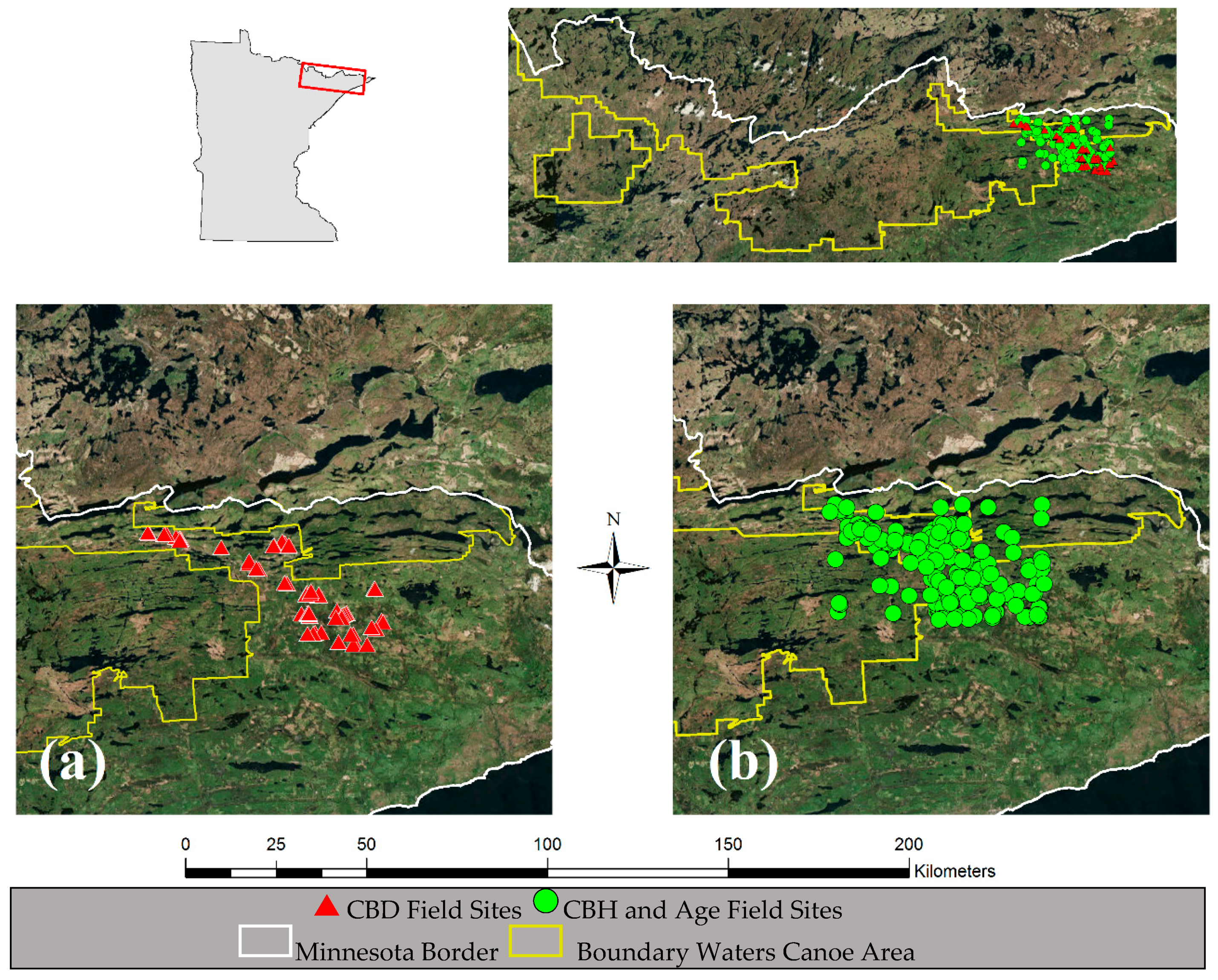
The study area covers 14,000 km2 in northern Minnesota, USA (Figure 1) and encompasses the Boundary Waters Canoe Area (BWCA). Elevation ranges from 337 to 701 m above mean sea-level. Pleistocene glacial till formed much of the soil structure in the BWCA with mineral soil conditions ranging from granitic deposits to sandy loams [11]. Because it is located in a transition zone between deciduous hardwoods and true northern boreal forests, the vegetation and biophysical characteristics of the BWCA are diverse. Conifers and deciduous tree species exist along a spectrum between pure and mixed stands of pines (Red, White, Jack), Balsam fir, Quaking aspen, Northern white cedar, maple (Red and Sugar), birch (Paper, Yellow), and spruce (White and Black). Recent fire history (1984–present) has included multiple large-scale events affecting a total of over 900 km2 of forested land in the BWCA and adjacent communities.
2.2. Sampling Design and Data Collection
Fuels data for CBH and age were collected at 263 inventory plots during an earlier, smaller pilot study area during the summers of 2014 and 2015 near a section of the Gunflint Trail. Plot locations were originally located using a stratified random sampling design, where strata were defined by forest types and stand age classes. These classes were composed of tree species commonly found across the greater extent of the BWCA, including: Jack, Red, and White pine, Black Spruce, Balsam fir, Paper birch, Quaking aspen. Plot locations were randomized within known forest stands >30 years old and >4.05 ha (10 acres). No plots were allowed within 24 m (80 ft) of a stand boundary or another plot. Forest inventory crews installed 0.04 ha (1/10th acre) fixed-radius forest inventory plots and recorded standard forest inventory data (i.e., individual tree measurements of species, height, and DBH) and additional plot-level measurements of stand age and canopy base height. Plots were located on the ground using handheld Trimble Juno GPS devices and differentially corrected to enhance the accuracy (2 to 5 m) of final plot locations. For this study, stand age was determined by selecting and coring the oldest tree from the dominant species present on each plot. CBH was assessed by two separate metrics: crown fuel base height (CFBH) and live crown base height (LCBH). Though these metrics subject to varying methodologies in other data collections, CFBH was here measured as the of height above the ground of the lowest live and/or dead fuels that can move fire higher in the tree. LCBH was determined by measuring the height above ground to the base of the live crown.
For CBD, a separate sample of 60 inventory plots were surveyed in 2015 and 2016. These plots were randomly located within the study area but within 2 km of a paved road and within a forested area. Plots were located on the ground using handheld Trimble GeoXT GPS devices and differentially corrected. At each plot, field crews recorded average canopy gap fraction (CGF), average and total species basal area, and average canopy height. A LAI-2200C instrument (LI-COR Biosciences, Lincoln, NE) was used to record CGF in a square 3 × 3 grid of nine points arranged around the plot center, each separated by five meters, following Reference [58]. With the LAI-2200C, a 38° angle was used with average canopy height to determine the respective CGF plot radius. Within this CGF-defined circular plot area, all conifers species >15 cm DBH were measured for height, height to first live branch, and canopy diameter. These data were used with published allometry [59] to calculate component biomass estimates for each field plot (i.e., needles, branch, and bole). The variety and detail of these measurements (i.e., biomass, CGF) allowed for the use and comparison of five CBD estimation methods (Table 1). These methods provide only indirect estimates and none are universally applicable to every forest type. Therefore, to determine the most appropriate CBD estimation method, only the most accurate of the five different methods tested was retained by comparing R2 and RMSE values.
2.3. Remote Sensing Data
Discrete-return LiDAR data used in the study was collected 14 May to 1 June 2011 by Woolpert, Inc. under contract from the State of Minnesota as a part of the Minnesota Elevation Mapping Project (MEMP). The expected outcome of the MEMP was the development of a state-wide, high-accuracy surface elevation dataset with possible vegetation mapping applications left unexplored. Horizontal positional accuracy of the dataset is ±1.6 m (α = 0.05) and vertical positional accuracy is 3.6 cm (α = 0.05) with a variable pulse return rate (depending on intercepted vegetation and topography), minimum side-lap of 25% and a scan angle of ± 20° off nadir [60]. The average density of the LiDAR point cloud is 0.44 pts/m2.
To characterize the horizontal and vertical distribution of vegetation a suite of raster grid metrics were created from the LiDAR point cloud data (Table 2) using the FUSION software package [61] at a 10 m spatial resolution. Due to the narrow side lap in the flight path and large scan angle, all potential predictors from FUSION metrics were visually screened for data quality issues before inclusion in the final predictor list. For example, canopy cover layers derived by FUSION due to excessive striping between flight lines and were replaced by a Landsat time-series derived canopy cover product [62]. For this replacement data, spectral indices were harmonized across all Landsat sensors along with photo-interpreted samples of canopy cover to produce annual maps of predicted canopy cover across the state from 1973–2015 [62]. The map of canopy cover for 2011 was chosen for use in all models to best match the year of LiDAR data collection. Finally, to synchronize predictor spatial resolutions, the Landsat-derived product was resampled from 30 m to a 10 m spatial resolution.
2.4. Model Development
A randomForest [63] k-nearest neighbor imputation approach (RF-kNN), available in the “yaImpute” R package [64], was used to develop models of four canopy fuel attributes: stand age, CFBH, LCBH, and CBD. RF-kNN is different from other imputation methods because it identifies nearest neighbor distances based on proximity values generated from an initial RF model [36]. Furthermore, comparative studies of nearest neighbor methods have shown RF-kNN to be a preferable modeling approach when predicting forest attributes [36,65,66,67,68,69,70].
Following previous work [42], model parsimony was optimized during the implementation of the RF-kNN approach to maximize the ecological interpretability of the model results. First, using the ‘rfUtilities’ package in R [71], a Gram–Schmidt QR decomposition was performed to identify and remove multicollinear variables. Next, to generate parsimonious RF models, an iterative selection function was performed using the ‘modelSel’ function in the ‘rfUtilities’ package [72]. This function generates a Model Improvement Ratio (MIR) statistic that describes how well predictor variables minimize the mean squared error and maximize the variation explained in the response. The RF model generating the highest MIR values is then identified as the most parsimonious model.
Using parsimony optimized predictor sets and associated RF proximity values, k-nearest neighbor imputations were run to generate predicted values to compare against the training data for LCBH, CFBH, CBD, and stand age. For the imputations, the number of neighbors was set to k = 1, a value understood to preserve the distribution and covariance structure of the reference dataset [73] and restrict the range of possible imputed values to that of the field data [36]. Canopy fuel attributes were then imputed across the study area at a 10 m spatial resolution.
2.5. Model Performance and Evaluation
The performance of each model was assessed by comparing imputed predictions to observed values in the training dataset and evaluating accuracy using an adjusted coefficient of determination (Adj. R2) and root mean square error (RMSE). The five methods of estimating CBD were analyzed and the method that produced the highest R2 and lowest RMSE value was retained as the final CBD model.
The influence of individual predictors in each model were analyzed in two ways. First, internal RF variable importance was generated to measure the mean decrease in model accuracy. Second, partial dependence plots were generated for the most important predictors in each model. In the context of RF modeling, partial dependence plots represent an attempt to visualize the relationship between the response variable and the marginal effect of a single predictor while accounting for the average effect of all other predictors used to grow the forest of regression trees [74,75].
3. Results
3.1. Model Selection and Variable Importance
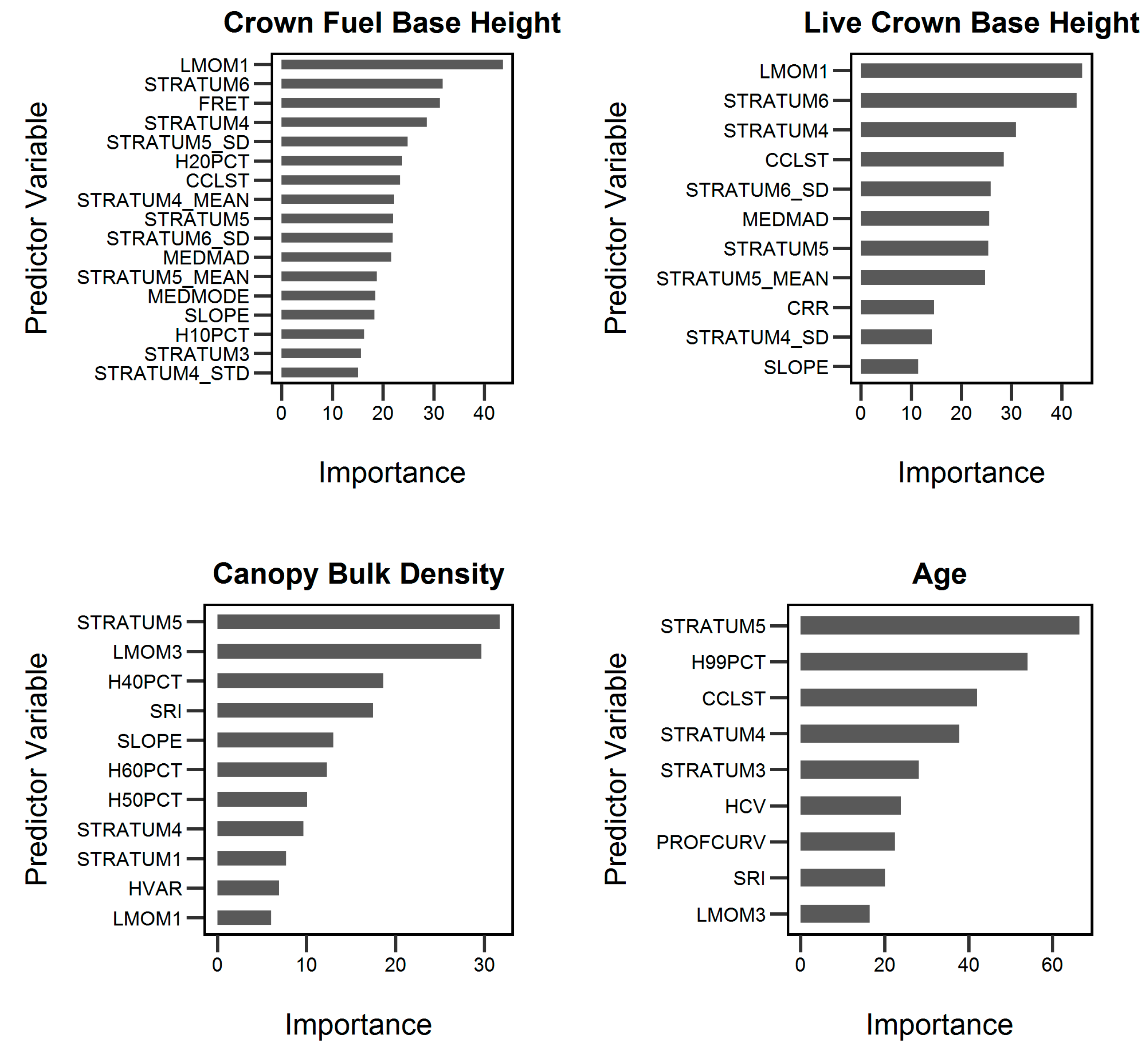
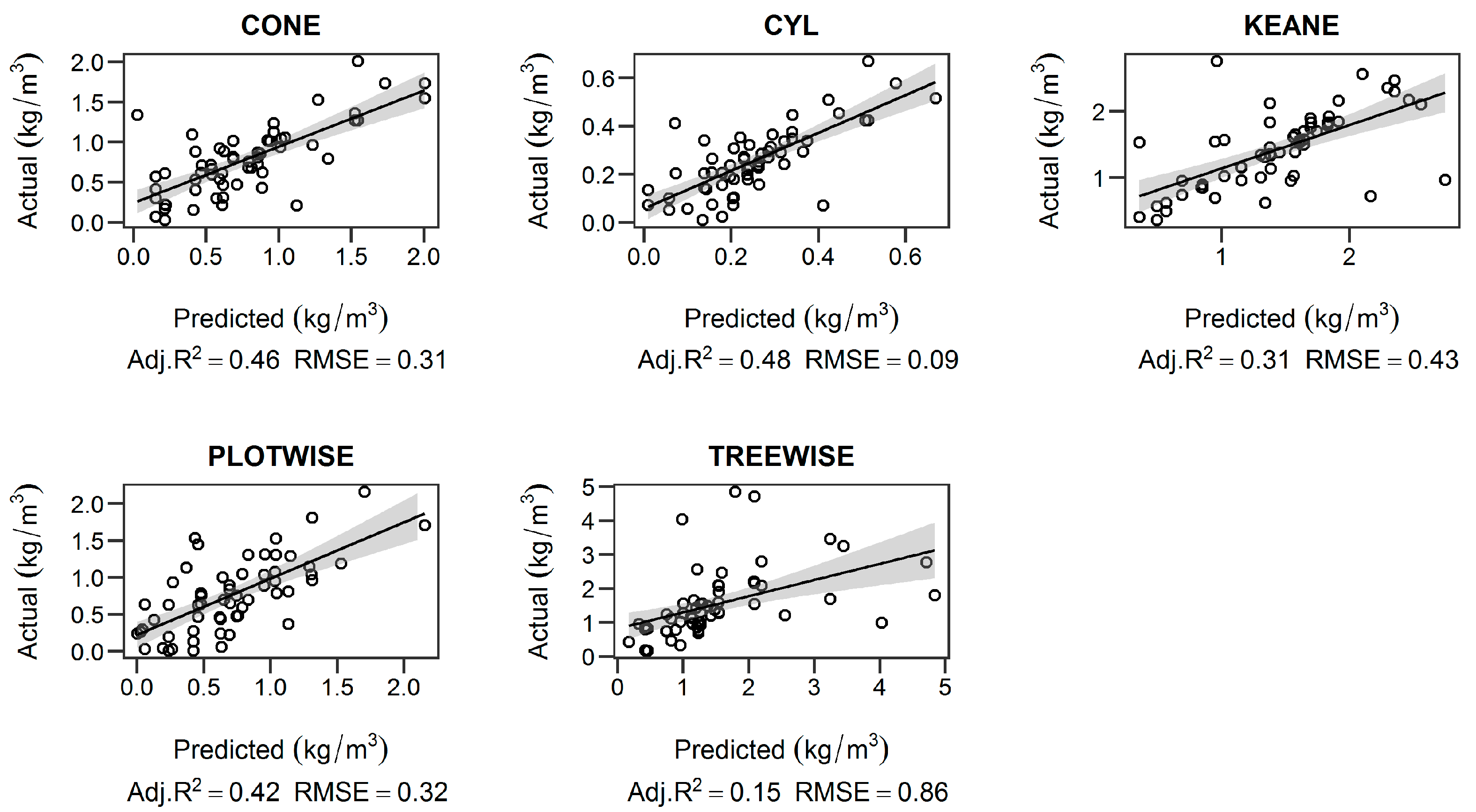
The QR-Decomposition procedure identified and removed 13 multicolinear predictors (Table 2), leaving 42 potential model metrics to use in model selection. The stand age model retained 9 predictors (Figure 2): mid-canopy pulse densities (STRATUM3, STRATUM4, STRATUM5), return heights (H99PCT, HCV), and surface texture (SRI, PROFCURV), as well as the Landsat time-series derived canopy cover layer (CCLST) and one L-moment (LMOM3). The CFBH model retained 17 predictors (Figure 2): the first L-moment, mid-canopy pulse densities (STRATUM3, STRATUM4, STRATUM5, STRATUM6), and return heights (H10PCT, H20PCT), among others (Table 2). The LCBH model retained 11 predictors (Figure 2): L-moments (LMOM1, LMOM3), mid-canopy pulse densities (STRATUM4, STRATUM5, STRATUM6), height distribution characteristics (MEDMAD, CRR), slope, and canopy cover (CCLST). Plot-wise cylinder volume (CYL; Table 1) was identified as the best candidate of the five CBD estimation methods (Figure 3) having a combination of the highest R2 and the lowest RMSE. The final CBD model retained 11 total predictors (Figure 2) including: mid-canopy pulse densities (STRATUM4, STRATUM5, STRATUM6), return heights (H40PCT, H50PCT, H60PCT, HVAR), surface texture (SRI), slope, and L-moments (LMOM1, LMOM3).
In terms of variable importance, the proportion of fifth strata returns (STRATUM5) and average return heights in the 99th percentile (H99PCT) were the most important for the stand age model (Figure 2). In the CBD model, the most important predictors (Figure 2) were the percentage of returns in the fifth strata (between 5 and 10 m) and the third L-moment (LMOM3). For the CFBH and LCBH models, the most important predictors (Figure 2) were identical: the proportion of returns from the sixth strata (STRATUM6) and the first L-moment (LMOM1).
3.2. Model Performance and Evaluation
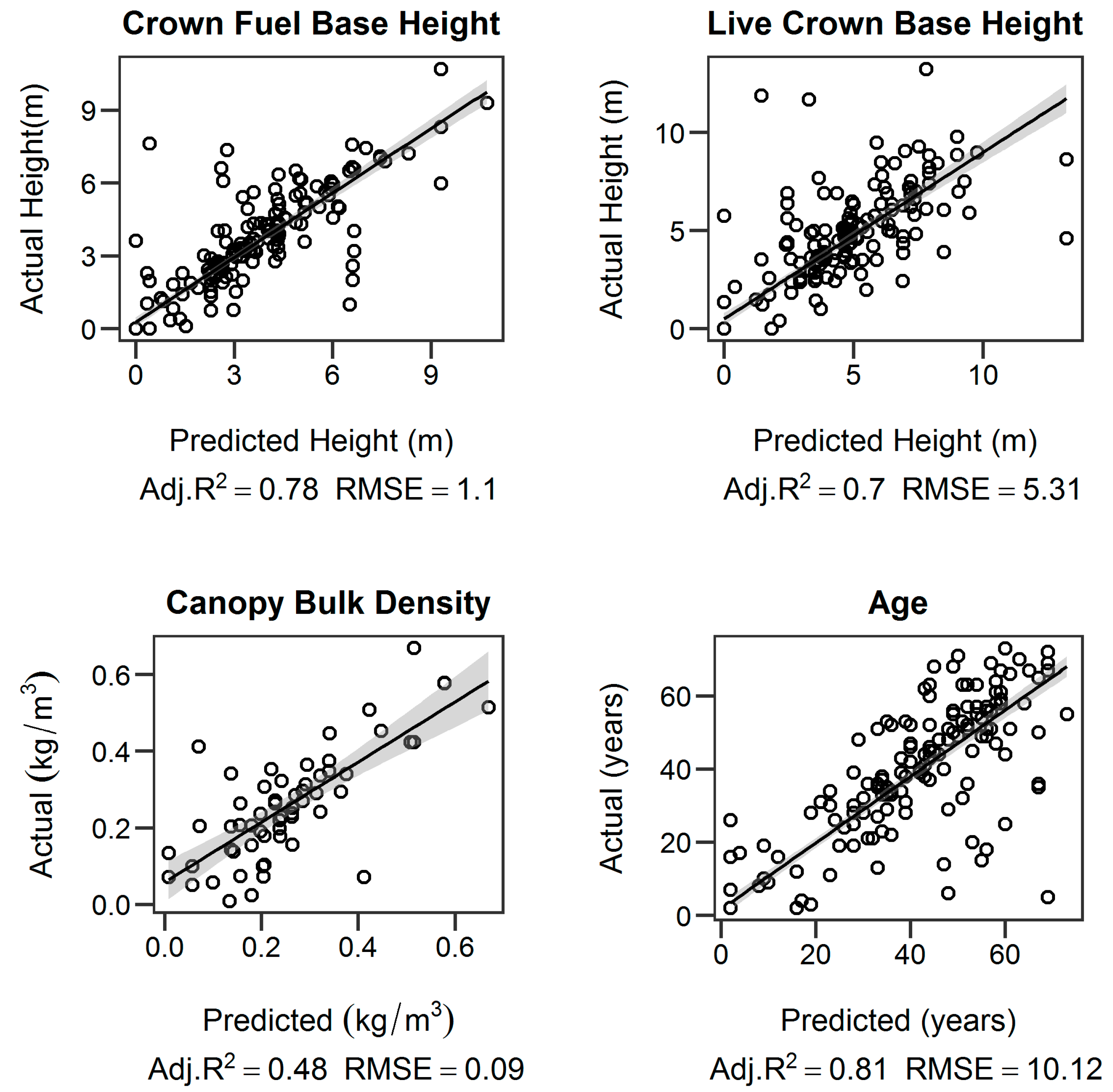
Overall, the imputation models of canopy fuels showed strong relationships (Figure 4) between predicted and field plot data for stand age (Adj. R2 = 0.81, RMSE = 10.12 years), CFBH (Adj. R2= 0.78, RMSE = 1.10 m), LCBH (Adj. R2= 0.7, RMSE = 1.60 m), and CBD (Adj. R2= 0.48, RMSE = 0.09 kg/m3).
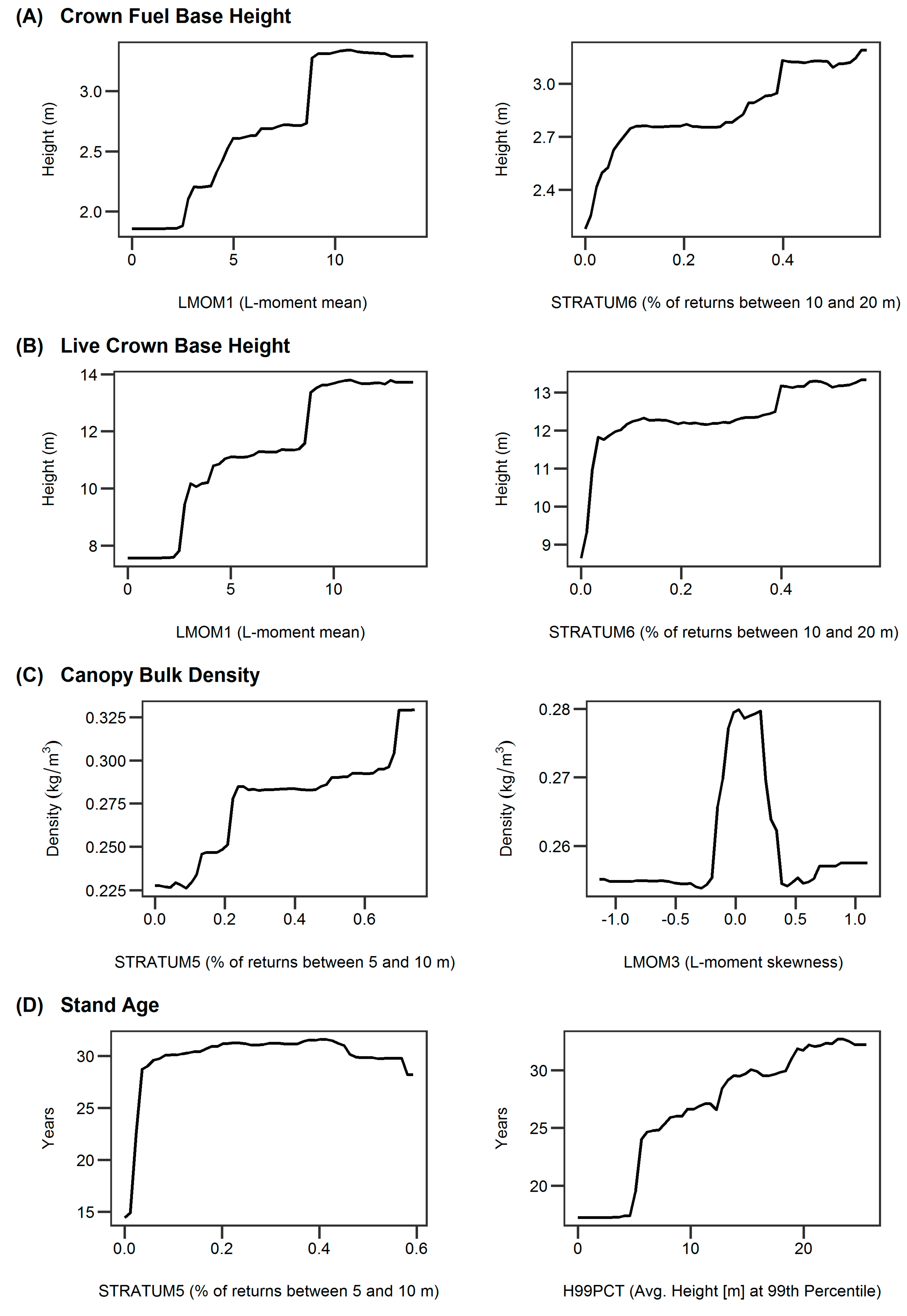
To determine the marginal effect of important variables (as determined by RF), partial dependence plots were examined for each canopy fuel attribute model. For the CFBH and LCBH models, the first L-moment (LMOM1) values and the proportion of sixth strata returns (STRATUM6) are both associated with increasing heights (Figure 5). For the CBD model, STRATUM5 values are associated with increasing biomass volumes while third L-moment (LMOM3) is associated with higher biomass volumes for values from ~ −0.5 to 0.5 (Figure 5). For the stand age model, the proportion of fifth strata returns (STRATUM5) are associated with variations in older stand ages while 99th percentile return heights (H99PCT) are associated with increasing stand ages (Figure 5).
4. Discussion
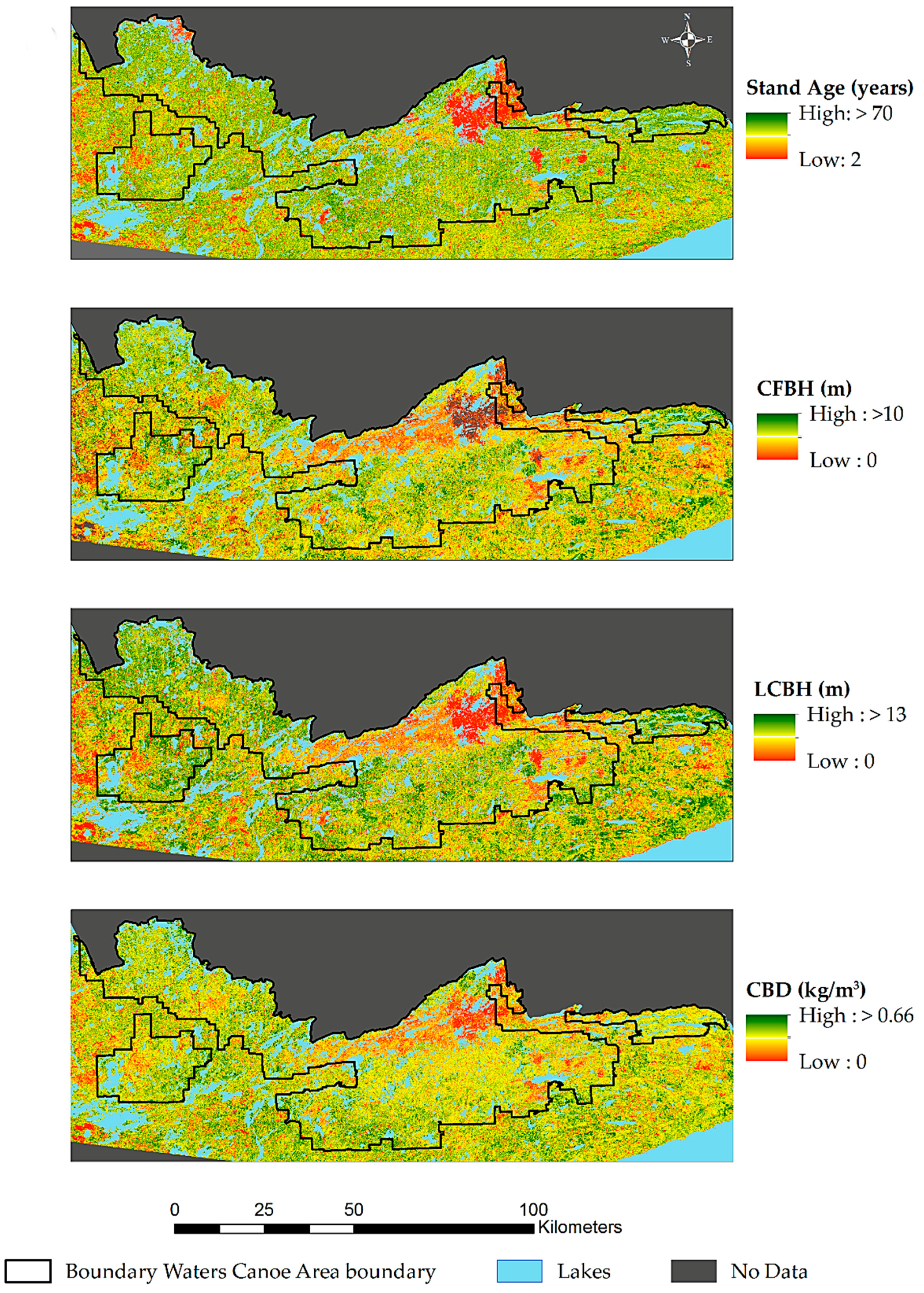
The RF-kNN models developed in this study demonstrate the ability of low-density LiDAR to effectively describe several canopy fuels attributes in a mixed forest setting. Imputed estimates of CFBH, LCBH, CBD, and stand age facilitated the production of detailed, 10 m spatial resolution maps (Figure 6) ready for use as fire behavior model inputs. The imputed products provide high accuracy, high spatial resolution alternatives to canopy fuels data sources (i.e., LANDFIRE) currently utilized by forest managers in the BWCA.
The accuracies presented in this study offer similar results compared to the few previous studies estimating CBH and CBD using low-density LiDAR (<1 pts/m2). For example, Maguya et al. [76] presented R2 values ranging from 0.46 to 0.75 for CBH at a point density of 0.5 pts/m2 in conifer-dominated forests of eastern Finland. Also using 0.5 pts/m2 point density, González-Ferreiro et al. [48] generated estimates for CBD (R2 = 0.44) but also reported CBH accuracy in upwards of R2 = 0.96 over plantations of young, highly stocked Pinus radiata in northwest Spain. Using LiDAR pulse densities much higher than those presented here, Andersen et al. [77] attained an R2 of 0.77 when estimating CBH from LiDAR data with a point density of 3.5 pts/m2 for a small forest in southwestern Washington dominated by Douglas fir (Pseudotsuga menziesii). In Douglas fir forest, Hermosilla et al. [44] achieved similar CBH results were achieved in in northwestern Oregon (R2: 0.78) using LiDAR with a point density of 8 pts/m2. Moreover, in the eastern Cascade mountains of Washington, accuracies ranging from R2 = 0.77 to 0.84 were reported by Erdody and Moskal [43] for CBH using a LiDAR dataset with a point density of 4 pts/m2. Finally, a study of forest age by Racine et al. [51] found comparable accuracy (R2: 0.83) using a similar a model methodology (RF-kNN imputation) and study system (northern boreal transition forest in Quebec, Canada). However, it should be noted that direct comparisons to these and other studies warrants caution due to differences in forest types, response variables (i.e., categorized age classes) and the use of square root and log transformations of dependent variables.
Using an RF-kNN imputation approach provides for the assessment of RF model predictor importance as measured by the normalized difference mean squared error ([78], Figure 2). Of the original 55 predictor variables, only one, describing the proportion of returns between 5 and 10 m (STRATUM5), was retained across all models. This finding is consistent with previous studies that have previously identified canopy strata return proportions as important across multiple models of forest attributes [79,80]. For the models of CFBH and LCBH, the most important variables are identical (LMOM1, STRATUM6). Similar marginal effects of each predictor are found in the partial dependence plots for the CFBH and LCBH models (Figure 5), where the importance of STRATUM6 (pulse density proportion between 10 and 20 m) can be explained by many CFBH and LCBH values falling within the height range of this strata. Despite being important in both models, STRATUM6 has different ecological implications for each model. This predictor becomes important for CFBH at lower heights and may reflect how the field measurements are better estimates of ladder fuels. In LCBH model, STRATUM6 explains greater variation mid-canopy heights, potentially indicating that this model will be less successful describing understory to crown fuel connectivity in fire behavior models.
The fact that LMOM1 was also shared by the CFBH and LCBH models is intriguing due to recent research regarding the improved understanding of forest structure through the use of L-moments [81]. The LMOM1 variable is functionally analogous to mean canopy height, a metric identified as an important component of other crown fuel models [19,43,44]. The efficacy of L-moments over conventional moments may be explained by the former’s robustness to the smaller sample sizes and outliers [82] such as those found in low-density LiDAR point cloud data.
For CBD, the top predictors were STRATUM5 and LMOM3 (an L-moment analogous to skewness). The partial dependence plot of CBD and STRATUM5 (Figure 5) indicates that the number of mid-canopy returns generally increases as the amount of tree biomass becomes denser between five and 10 meters above ground level. The plot of LMOM3 to CBD (Figure 5) indicates that increasing biomass volumes are associated with returns distributed mostly through the mid-crown heights. As the number of returns concentrate at either higher or lower heights, biomass values decrease. However, it should be noted that the variation of the marginal effect on CBD occurs over a narrow range (0.255 to 0.280 kg/m3). The CBD method with the highest model performance was “CYL”, which is designed to represent plotwise total CBD based on cylinder shapes of trees and assumes that biomass is distributed equally in the crown. Compared to the other tested methods (Table 1), the generic cylinder shape may have been more successful in capturing the variations in canopy profiles across a wide variety of deciduous and coniferous crown geometries.
For the stand age model, the most important predictors were STRATUM5 and H99PCT (the average height of the 99th percentile of returns). The known relationship between age and tree height [83] is supported by the importance of H99PCT in the stand age model and the association of H99PCT with increasing stand ages in the partial dependence plot (Figure 5). The partial dependence plot for STRATUM5 and stand age (Figure 5) appears to indicate the power of this predictor lies mainly in its ability to distinguish between zero and non-zero values of stand age, which potentially translates to forested vs. non-forested conditions. Predicted non-forested conditions may also encompass emergent vegetation (i.e., fire recovery) or highlight potential replanting or restocking areas. It must be said that stand age is not requisite in standard fire behavior modeling software. Despite this, spatial predictions of forest age classes provide valuable information beyond fire assessment alone. For example, paired with forest type classifications, stand age classes can highlight varying habitat suitability for wildlife species or provide potential context to stand-level impacts of other ecological process such as water transport and carbon sequestration.
Despite numerous studies of forest attributes using LiDAR, previous research has focused heavily on conifer-dominated systems [84]. This may be partially driven by concerns over the variability of leaf-off, leaf-on conditions in forests with deciduous components or a concentration of research in locations with available funding for LiDAR data collection efforts. However, previous research has shown that the timing of LiDAR acquisition has only a marginal effect on the accuracy of modeled biophysical forest structure estimates [85,86,87], which is notable since LiDAR collections occur across a wide variety of forest conditions in the BWCA. Beyond the BWCA, data covering mixed forest systems have been used to estimate forest biomass [84,88,89,90], stem density [91], and basal area [92,93] and results from this study contribute to this underrepresented body of work.
Characterizations of canopy structure have shown only small differences in accuracy and precision between high and low-density LiDAR collections [55,94,95]. However, the use of low-density scenarios using simulated point clouds thinned from high-density datasets [94] may lack the real-world collection parameters presented here (i.e., low side-lap, high scan angle). This study’s use of unsimulated data shows the added benefit of a LiDAR collection even when the original acquisition plans do not specifically include vegetation mapping (as was the case with the Minnesota Elevation Mapping Project). As of April 2019, low-density LiDAR covers 64% of the land area in the continental United States [57] and presents a cost-effective and readily available complement to expensive, time-consuming, and logistically complex field-based sampling. And although there is some temporal difference between the timing of the LiDAR collection and the field data observations, the field data extent did not experience large shifts in vegetation or habitat type during the intervening years, allowing these model outputs to be useful for fire ecologists and forest managers. Going forward, managers may be able to use landscape altering events (i.e., fire, blowdown) occurring after 2015 to help validate or update the model outputs.
Although direct comparisons should be used with caution, it is worth noting the model accuracies produced in this study meet or surpass those of commonly utilized canopy fuels estimates of from LANDFIRE for CBH (R2 = 0.48) and CBD (R2 = 0.58) in the Lake States region, Zone 41 [96]. However, several caveats are needed to contextualize LANDFIRE data. First, accuracy estimates are generated across much larger geographic areas due to sample size and distribution issues at smaller extents [96]. Second, CBH products from LANDFIRE are defined as “the lowest layer in the canopy at which the CBD is ≥ 0.012 kg m3” [26] and are therefore more analogous to the CFBH than LCBH metric presented here. The latter was concurrently measured and estimated to provide the USFS with differing inputs for comparative models of fire risk. Lastly, despite the difficulty in direct comparisons between LANDFIRE and independent field measurement [26], it notable that CBH and CBD data from LANDFIRE were poorly correlated with the field data used in this study (R2 range: 0.01 - 0.30). The difference in accuracy can be explained by LiDAR’s ability to describe the three-dimensional structure of forest canopies, whereas LANDFIRE is reliant on two-dimensional, optical satellite sensor data, such as Landsat (30 m spatial resolution). High spatial resolution data from LiDAR also leads to more detailed spatial inputs for fire modeling and more relevant information for local, operational forest management.
The results of this study demonstrate the utility of low-density LiDAR, but it is worth pointing out that two aspects of the initial data collection effort may have hindered model performance. The LiDAR data was collected with a minimum side-lap of 25%, which is less than the 50% often seen in other collection efforts. Low or inconsistent side-lap can influence overall point densities. The wide scan angle of the LiDAR collection (20 degrees) may have also led to the striping seen during the initial visual assessment of the potential predictors because larger off-nadir angles can affect the proportion of canopy returns [97]. The negative effects of inconsistent side-lap and variable scan patterns are much more difficult to mitigate using common thinning algorithms in low density point cloud data, but the CCLST predictor proved a sufficient supplement and improved model performance in some cases. Going forward, related research [98,99,100] indicates that fusing Landsat time-series data and LiDAR metrics should be further explored to test the efficacy of low-density LiDAR. Finally, though the model outputs presented here represent extrapolations outside the geographic extent of the original field data collection sites, the imputation parameters are bounded to the range of field data. These results represent specific associations between spatial predictors and forest measurements and may not fully capture novel ecological conditions across the continuum of the BWCA. Thus, these models should not be seen as transferable to forest types with significant differences in species composition, phenology, or topography.
5. Conclusions
This study demonstrates that low-density LiDAR can be used to provide reasonable estimates of canopy fuel attributes in the mixed forest ecosystem of northern Minnesota, USA. The results also highlight the use of pre-existing low-density LiDAR collections to complement the limited resources of forest managers to gather plot-based field data. The map products of imputed canopy fuel attributes produced by this study are of higher spatial resolution (10 m) relative to similar products from national data repositories, such as LANDFIRE. They can serve as alternative or improved inputs for forest managers in comparative model scenarios of fire behavior and risk. It is encouraging that the data limitations of low-density LiDAR were generally not a major hindrance to model accuracy. These results indicate the expanded utility of low-density LiDAR and suggest re-evaluations of the large number of similar datasets available across the United States.
Author Contributions
Conceptualization, P.J., M.F., A.P.; Methodology, P.W., A.P., P.S.E.; Formal Analysis, P.E.; Data Curation, P.S.E.; Writing-Original Draft Preparation, P.S.E.; Writing-Review & Editing, P.S.E., M.J.F., P.W., A.P., P.J.; Visualization, P.S.E.; Supervision, M.J.F.; Project Administration, M.J.F.; Funding Acquisition, P.J. and M.J.F.
Funding
This research was funded by the US Forest Service Superior National Forest.
Acknowledgments
The authors would like to acknowledge Steve Filippelli for his expertise with LiDAR and geospatial programming.
Conflicts of Interest
The authors declare no conflict of interest.
References
- Agee, J.K.; Skinner, C.N. Basic principles of forest fuel reduction treatments. For. Ecol. Manag. 2005, 211, 83–96. [Google Scholar] [CrossRef]
- Keane, R.E.; Ryan, K.C.; Veblen, T.T.; Allen, C.D.; Logan, J.; Hawkes, B. Cascading effects of fire exclusion in the Rocky Mountain ecosystems: a literature review; U.S. Department of Agriculture, Forest Service, Rocky Mountain Research Station: Fort Collins, CO, USA, 2002. [Google Scholar]
- Balch, J.K.; Bradley, B.A.; Abatzoglou, J.T.; Nagy, R.C.; Fusco, E.J.; Mahood, A.L. Human-started wildfires expand the fire niche across the United States. Proc. Natl. Acad. Sci. USA 2017, 114, 2946–2951. [Google Scholar] [CrossRef] [PubMed] [Green Version]
- Nagy, R.C.; Fusco, E.; Bradley, B.; Abatzoglou, J.T.; Balch, J. Human-Related Ignitions Increase the Number of Large Wildfires across U.S. Ecoregions. Fire 2018, 1, 4. [Google Scholar] [CrossRef]
- Radeloff, V.C.; Helmers, D.P.; Kramer, H.A.; Mockrin, M.H.; Alexandre, P.M.; Bar-Massada, A.; Butsic, V.; Hawbaker, T.J.; Martinuzzi, S.; Syphard, A.D.; et al. Rapid growth of the US wildland-urban interface raises wildfire risk. Proc. Natl. Acad. Sci. USA 2018, 115, 3314–3319. [Google Scholar] [CrossRef] [PubMed] [Green Version]
- Van Mantgem, P.J.; Nesmith, J.C.B.; Keifer, M.; Knapp, E.E.; Flint, A.; Flint, L. Climatic stress increases forest fire severity across the western United States. Ecol. Lett. 2013, 16, 1151–1156. [Google Scholar] [CrossRef]
- Westerling, A.L.; Hidalgo, H.G.; Cayan, D.R.; Swetnam, T.W. Warming and Earlier Spring Increase Western U.S. Forest Wildfire Activity. Science 2006, 313, 940–943. [Google Scholar] [CrossRef] [Green Version]
- Westerling Anthony LeRoy Increasing western US forest wildfire activity: sensitivity to changes in the timing of spring. Philos. Trans. R. Soc. B Biol. Sci. 2016, 371, 20150178. [CrossRef]
- Littell, J.S.; Peterson, D.L.; Riley, K.L.; Liu, Y.; Luce, C.H. A review of the relationships between drought and forest fire in the United States. Glob. Change Biol. 2016, 22, 2353–2369. [Google Scholar] [CrossRef]
- Swain, A.M. A History of Fire and Vegetation in Northeastern Minnesota as Recorded in Lake Sediments. Quat. Res. 1973, 3, 383–396. [Google Scholar] [CrossRef]
- Heinselman, M.L. The Boundary Waters Wilderness Ecosystem; 1. paperback print; Univ. of Minnesota Press: Minneapolis, MN, USA, 1999; ISBN 978-0-8166-2805-6. [Google Scholar]
- USFS (United States Forest Service) Pagami Creek Fire Face Sheet. Available online: https://www.fs.usda.gov/Internet/FSE_DOCUMENTS/stelprdb5346343.pdf (accessed on 14 June 2019).
- Ashley, W.S.; Mote, T.L. Derecho Hazards in the United States. Bull. Am. Meteorol. Soc. 2005, 86, 1577–1592. [Google Scholar] [CrossRef]
- National Interagency Fire Center (NIFC). Federal Firefighting Costs (Suppression Only); National Interagency Fire Center: Boise, ID, USA, 2018. [Google Scholar]
- Finney, M.A. FARSITE: Fire Area Simulator-model development and evaluation; U.S. Department of Agriculture, Forest Service, Rocky Mountain Research Station: Fort Collins, CO, USA, 1998.
- Finney, M.A. An overview of FlamMap fire modeling capabilities. In Proceedings of the Proceedings RMRS-P-41: Fuels Management—How to Measure Success, Portland, OR, USA, 28–30 March 2006; U.S. Department of Agriculture, Forest Service, Rocky Mountain Research Station: Fort Collins, CO, USA, 2006; pp. 213–220. [Google Scholar]
- Keane, R.E.; Burgan, R.; van Wagtendonk, J. Mapping wildland fuels for fire management across multiple scales: Integrating remote sensing, GIS, and biophysical modeling. Int. J. Wildland Fire 2001, 10, 301–319. [Google Scholar] [CrossRef]
- Scott, J.H.; Reinhardt, E.D. Assessing Crown Fire Potential by Linking Models of Surface and Crown Fire Behavior; U.S. Department of Agriculture, Forest Service, Rocky Mountain Research Station: Fort Collins, CO, USA, 2001.
- Riaño, D.; Chuvieco, E.; Condés, S.; González-Matesanz, J.; Ustin, S.L. Generation of crown bulk density for Pinus sylvestris L. from lidar. Remote Sens. Environ. 2004, 92, 345–352. [Google Scholar] [CrossRef]
- Tiribelli, F.; Kitzberger, T.; Morales, J.M. Changes in vegetation structure and fuel characteristics along post-fire succession promote alternative stable states and positive fire–vegetation feedbacks. J. Veg. Sci. 2018, 29, 147–156. [Google Scholar] [CrossRef]
- Erni, S.; Arseneault, D.; Parisien, M.-A. Stand Age Influence on Potential Wildfire Ignition and Spread in the Boreal Forest of Northeastern Canada. Ecosystems 2018, 21, 1471–1486. [Google Scholar] [CrossRef]
- Wood, J.D.; Cohen, B.S.; Prebyl, T.J.; Conner, L.M.; Collier, B.A.; Chamberlain, M.J. Time-since-fire and stand seral stage affect habitat selection of eastern wild turkeys in a managed longleaf pine ecosystem. For. Ecol. Manag. 2018, 411, 203–212. [Google Scholar] [CrossRef]
- Kalamees, R.; Püssa, K.; Vanha-Majamaa, I.; Zobel, K. The effects of fire and stand age on seedling establishment of Pulsatilla patens in a pine-dominated boreal forest. Can. J. Bot. 2005, 83, 688–693. [Google Scholar] [CrossRef]
- Taylor, C.; McCarthy, M.A.; Lindenmayer, D.B. Nonlinear Effects of Stand Age on Fire Severity. Conserv. Lett. 2014, 7, 355–370. [Google Scholar] [CrossRef] [Green Version]
- Rollins, M.G. LANDFIRE: A nationally consistent vegetation, wildland fire, and fuel assessment. Int. J. Wildland Fire 2009, 18, 235–249. [Google Scholar] [CrossRef]
- Reeves, M.C.; Kost, J.R.; Ryan, K.C. Fuels Products of the LANDFIRE Project. In Proceedings of the USDA Forest Service Proceedings RMRS-P-41, Portland, OR, USA, 26–30 March 2006; USDA Forest Service: Fort Collins, CO, USA, 2006; pp. 239–252. [Google Scholar]
- Krasnow, K.; Schoennagel, T.; Veblen, T.T. Forest fuel mapping and evaluation of LANDFIRE fuel maps in Boulder County, Colorado, USA. For. Ecol. Manag. 2009, 257, 1603–1612. [Google Scholar] [CrossRef]
- Pierce, A.D.; Farris, C.A.; Taylor, A.H. Use of random forests for modeling and mapping forest canopy fuels for fire behavior analysis in Lassen Volcanic National Park, California, USA. For. Ecol. Manag. 2012, 279, 77–89. [Google Scholar] [CrossRef]
- Reeves, M.C.; Ryan, K.C.; Rollins, M.G.; Thompson, T.G. Spatial fuel data products of the LANDFIRE Project. Int. J. Wildland Fire 2009, 18, 250–267. [Google Scholar] [CrossRef]
- Lefsky, M.A.; Cohen, W.B.; Spies, T.A. An evaluation of alternate remote sensing products for forest inventory, monitoring, and mapping of Douglas-fir forests in western Oregon. Can. J. For. Res. 2001, 31, 78–87. [Google Scholar] [CrossRef]
- Wagner, W.; Hollaus, M.; Briese, C.; Ducic, V. 3D vegetation mapping using small-footprint full-waveform airborne laser scanners. Int. J. Remote Sens. 2008, 29, 1433–1452. [Google Scholar] [CrossRef]
- Lefsky, M.A.; Harding, D.; Cohen, W.B.; Parker, G.; Shugart, H.H. Surface Lidar Remote Sensing of Basal Area and Biomass in Deciduous Forests of Eastern Maryland, USA. Remote Sens. Environ. 1999, 67, 83–98. [Google Scholar] [CrossRef]
- Falkowski, M.J.; Hudak, A.T.; Crookston, N.L.; Gessler, P.E.; Uebler, E.H.; Smith, A.M.S. Landscape-scale parameterization of a tree-level forest growth model: A k-nearest neighbor imputation approach incorporating LiDAR data. Can. J. For. Res. 2010, 40, 184–199. [Google Scholar] [CrossRef]
- Fekety, P.A.; Falkowski, M.J.; Hudak, A.T. Temporal transferability of LiDAR-based imputation of forest inventory attributes. Can. J. For. Res. 2014, 45, 422–435. [Google Scholar] [CrossRef]
- Hudak, A.T.; Crookston, N.L.; Evans, J.S.; Falkowski, M.J.; Smith, A.M.S.; Gessler, P.E.; Morgan, P. Regression modeling and mapping of coniferous forest basal area and tree density from discrete-return lidar and multispectral satellite data. Can. J. Remote Sens. 2006, 32, 126–138. [Google Scholar] [CrossRef]
- Hudak, A.T.; Crookston, N.L.; Evans, J.S.; Hall, D.E.; Falkowski, M.J. Nearest neighbor imputation of species-level, plot-scale forest structure attributes from LiDAR data. Remote Sens. Environ. 2008, 112, 2232–2245. [Google Scholar] [CrossRef] [Green Version]
- Boudreau, J.; Nelson, R.F.; Margolis, H.A.; Beaudoin, A.; Guindon, L.; Kimes, D.S. Regional aboveground forest biomass using airborne and spaceborne LiDAR in Québec. Remote Sens. Environ. 2008, 112, 3876–3890. [Google Scholar] [CrossRef]
- Zhao, K.; Popescu, S.; Nelson, R. Lidar remote sensing of forest biomass: A scale-invariant estimation approach using airborne lasers. Remote Sens. Environ. 2009, 113, 182–196. [Google Scholar] [CrossRef]
- Morsdorf, F.; Frey, O.; Meier, E.; Itten, K.I.; Allgöwer, B. Assessment of the influence of flying altitude and scan angle on biophysical vegetation products derived from airborne laser scanning. Int. J. Remote Sens. 2008, 29, 1387–1406. [Google Scholar] [CrossRef]
- Riaño, D.; Valladares, F.; Condés, S.; Chuvieco, E. Estimation of leaf area index and covered ground from airborne laser scanner (Lidar) in two contrasting forests. Agric. For. Meteorol. 2004, 124, 269–275. [Google Scholar] [CrossRef]
- Tang, H.; Brolly, M.; Zhao, F.; Strahler, A.H.; Schaaf, C.L.; Ganguly, S.; Zhang, G.; Dubayah, R. Deriving and validating Leaf Area Index (LAI) at multiple spatial scales through lidar remote sensing: A case study in Sierra National Forest, CA. Remote Sens. Environ. 2014, 143, 131–141. [Google Scholar] [CrossRef]
- Falkowski, M.J.; Evans, J.S.; Martinuzzi, S.; Gessler, P.E.; Hudak, A.T. Characterizing forest succession with lidar data: An evaluation for the Inland Northwest, USA. Remote Sens. Environ. 2009, 113, 946–956. [Google Scholar] [CrossRef] [Green Version]
- Erdody, T.L.; Moskal, L.M. Fusion of LiDAR and imagery for estimating forest canopy fuels. Remote Sens. Environ. 2010, 114, 725–737. [Google Scholar] [CrossRef]
- Hermosilla, T.; Ruiz, L.A.; Kazakova, A.N.; Coops, N.C.; Moskal, L.M. Estimation of forest structure and canopy fuel parameters from small-footprint full-waveform LiDAR data. Int. J. Wildland Fire 2014, 23, 224–233. [Google Scholar] [CrossRef] [Green Version]
- Skowronski, N.S.; Clark, K.L.; Duveneck, M.; Hom, J. Three-dimensional canopy fuel loading predicted using upward and downward sensing LiDAR systems. Remote Sens. Environ. 2011, 115, 703–714. [Google Scholar] [CrossRef]
- Popescu, S.C.; Zhao, K. A voxel-based lidar method for estimating crown base height for deciduous and pine trees. Remote Sens. Environ. 2008, 112, 767–781. [Google Scholar] [CrossRef]
- Zhao, K.; Popescu, S.; Meng, X.; Pang, Y.; Agca, M. Characterizing forest canopy structure with lidar composite metrics and machine learning. Remote Sens. Environ. 2011, 115, 1978–1996. [Google Scholar] [CrossRef]
- González-Ferreiro, E.; Diéguez-Aranda, U.; Crecente-Campo, F.; Barreiro-Fernández, L.; Miranda, D.; Castedo-Dorado, F. Modelling canopy fuel variables for Pinus radiata D. Don in NW Spain with low-density LiDAR data. Int. J. Wildland Fire 2014, 23, 350–362. [Google Scholar] [CrossRef]
- Hall, S.A.; Burke, I.C.; Box, D.O.; Kaufmann, M.R.; Stoker, J.M. Estimating stand structure using discrete-return lidar: an example from low density, fire prone ponderosa pine forests. For. Ecol. Manag. 2005, 208, 189–209. [Google Scholar] [CrossRef]
- Riaño, D.; Meier, E.; Allgöwer, B.; Chuvieco, E.; Ustin, S.L. Modeling airborne laser scanning data for the spatial generation of critical forest parameters in fire behavior modeling. Remote Sens. Environ. 2003, 86, 177–186. [Google Scholar] [CrossRef]
- Racine, E.B.; Coops, N.C.; St-Onge, B.; Bégin, J. Estimating Forest Stand Age from LiDAR-Derived Predictors and Nearest Neighbor Imputation. For. Sci. 2014, 60, 128–136. [Google Scholar] [CrossRef]
- Evans, J.; Hudak, A.; Faux, R.; Smith, A.M. Discrete Return Lidar in Natural Resources: Recommendations for Project Planning, Data Processing, and Deliverables. Remote Sens. 2009, 1, 776–794. [Google Scholar] [CrossRef] [Green Version]
- Montagnoli, A.; Fusco, S.; Terzaghi, M.; Kirschbaum, A.; Pflugmacher, D.; Cohen, W.B.; Scippa, G.S.; Chiatante, D. Estimating forest aboveground biomass by low density lidar data in mixed broad-leaved forests in the Italian Pre-Alps. For. Ecosyst. 2015, 2, 10. [Google Scholar] [CrossRef] [Green Version]
- Shendryk, I.; Hellström, M.; Klemedtsson, L.; Kljun, N. Low-Density LiDAR and Optical Imagery for Biomass Estimation over Boreal Forest in Sweden. Forests 2014, 5, 992–1010. [Google Scholar] [CrossRef]
- Treitz, P.; Lim, K.; Woods, M.; Pitt, D.; Nesbitt, D.; Etheridge, D. LiDAR Sampling Density for Forest Resource Inventories in Ontario, Canada. Remote Sens. 2012, 4, 830–848. [Google Scholar] [CrossRef] [Green Version]
- Thomas, V.; Treitz, P.; McCaughey, J.H.; Morrison, I. Mapping stand-level forest biophysical variables for a mixedwood boreal forest using lidar: An examination of scanning density. Can. J. For. Res. 2006, 36, 34–47. [Google Scholar] [CrossRef]
- Department of Commerce (DOC); National Oceanic and Atmospheric Administration (NOAA); National Ocean Service (NOS); Office for Coastal Management (OCM). United States Interagency Elevation Inventory (USIEI) Viewer—Topographic/Bathymetric Data. Available online: https://coast.noaa.gov/inventory (accessed on 2 March 2018).
- Keane, R.E.; Reinhardt, E.D.; Scott, J.; Gray, K.; Reardon, J. Estimating forest canopy bulk density using six indirect methods. Can. J. For. Res. 2005, 35, 724–739. [Google Scholar] [CrossRef]
- Perala, D.A.; Alban, D. Allometric Biomass Estimators for Aspen-Dominated Ecosystems in the Upper Great Lakes.; U.S. Department of Agriculture, Forest Service, North Central Research Station: St. Paul, MN, USA, 1993.
- MNGEO. LiDAR Elevation, Arrowhead Region, NE Minnesota. Available online: http://www.mngeo.state.mn.us/chouse/metadata/lidar_arrowhead2011.html (accessed on 17 December 2017).
- McGaughey, R.J. FUSION/LDV: software for LIDAR data analysis and visualization. USDA Forest Service. Pacific Northwest Research Station. Available online: http://forsys.sefs.uw.edu/fusion/fusionlatest.html (accessed on 1 February 2018).
- Vogeler, J.C.; Braaten, J.D.; Slesak, R.A.; Falkowski, M.J. Extracting the full value of the Landsat archive: Inter-sensor harmonization for the mapping of Minnesota forest canopy cover (1973–2015). Remote Sens. Environ. 2018, 209, 363–374. [Google Scholar] [CrossRef]
- Breiman, L. Random Forests. Mach. Learn. 2001, 45, 5–32. [Google Scholar] [CrossRef] [Green Version]
- Crookston, N.L.; Finley, A.O. yaImpute: An R Package for kNN Imputation. J. Stat. Softw. 2008, 23. [Google Scholar] [CrossRef]
- Eskelson, B.; Barrett, T.; Temesgen, H. Imputing mean annual change to estimate current forest attributes. Silva Fenn. 2009, 43. [Google Scholar] [CrossRef] [Green Version]
- Hudak, A.T.; Haren, A.T.; Crookston, N.L.; Liebermann, R.J.; Ohmann, J.L. Imputing Forest Structure Attributes from Stand Inventory and Remotely Sensed Data in Western Oregon, USA. For. Sci. 2014, 60, 253–269. [Google Scholar] [CrossRef] [Green Version]
- Latifi, H.; Koch, B. Evaluation of most similar neighbour and random forest methods for imputing forest inventory variables using data from target and auxiliary stands. Int. J. Remote Sens. 2012, 33, 6668–6694. [Google Scholar] [CrossRef]
- Latifi, H.; Nothdurft, A.; Koch, B. Non-parametric prediction and mapping of standing timber volume and biomass in a temperate forest: application of multiple optical/LiDAR-derived predictors. Forestry 2010, 83, 395–407. [Google Scholar] [CrossRef] [Green Version]
- Packalén, P.; Temesgen, H.; Maltamo, M. Variable selection strategies for nearest neighbor imputation methods used in remote sensing based forest inventory. Can. J. Remote Sens. 2012, 38, 557–569. [Google Scholar] [CrossRef]
- Powell, S.L.; Cohen, W.B.; Healey, S.P.; Kennedy, R.E.; Moisen, G.G.; Pierce, K.B.; Ohmann, J.L. Quantification of live aboveground forest biomass dynamics with Landsat time-series and field inventory data: A comparison of empirical modeling approaches. Remote Sens. Environ. 2010, 114, 1053–1068. [Google Scholar] [CrossRef]
- Evans, J.S.; Murphy, M.A.; Holden, Z.A.; Cushman, S.A. Modeling Species Distribution and Change Using Random Forest. In Predictive Species and Habitat Modeling in Landscape Ecology; Drew, C.A., Wiersma, Y.F., Huettmann, F., Eds.; Springer New York: New York, NY, USA, 2011; pp. 139–159. ISBN 978-1-4419-7389-4. [Google Scholar]
- Murphy, M.; Evans, J.; Storfer, A. Quantifying Bufo boreas connectivity in Yellowstone National Park with landscape genetics. Ecology 2010, 91, 252–261. [Google Scholar] [CrossRef] [Green Version]
- Franco-Lopez, H.; Ek, A.R.; Bauer, M.E. Estimation and mapping of forest stand density, volume, and cover type using the k-nearest neighbors method. Remote Sens. Environ. 2001, 77, 251–274. [Google Scholar] [CrossRef]
- Cafri, G.; Bailey, B.A. Understanding Variable Effects from Black Box Prediction: Quantifying Effects in Tree Ensembles Using Partial Dependence. J. Data Sci. 2016, 14, 67–96. [Google Scholar]
- Cutler, D.R.; Edwards, T.C.; Beard, K.H.; Cutler, A.; Hess, K.T.; Gibson, J.; Lawler, J.J. Random Forests for Classification in Ecology. Ecology 2007, 88, 2783–2792. [Google Scholar] [CrossRef] [PubMed]
- Maguya, A.S.; Tegel, K.; Junttila, V.; Kauranne, T.; Korhonen, M.; Burns, J.; Leppanen, V.; Sanz, B. Moving Voxel Method for Estimating Canopy Base Height from Airborne Laser Scanner Data. Remote Sens. 2015, 7, 8950–8972. [Google Scholar] [CrossRef] [Green Version]
- Andersen, H.-E.; McGaughey, R.J.; Reutebuch, S.E. Estimating forest canopy fuel parameters using LIDAR data. Remote Sens. Environ. 2005, 94, 441–449. [Google Scholar] [CrossRef]
- Liaw, A.; Wiener, M. Classification and Regression by randomForest. RNews 2002, 2, 5. [Google Scholar]
- Bright, B.C.; Hudak, A.T.; Meddens, A.J.H.; Hawbaker, T.J.; Briggs, J.S.; Kennedy, R.E. Prediction of Forest Canopy and Surface Fuels from Lidar and Satellite Time Series Data in a Bark Beetle-Affected Forest. Forests 2017, 8, 322. [Google Scholar] [CrossRef]
- González-Olabarria, J.-R.; Rodríguez, F.; Fernández-Landa, A.; Mola-Yudego, B. Mapping fire risk in the Model Forest of Urbión (Spain) based on airborne LiDAR measurements. For. Ecol. Manag. 2012, 282, 149–156. [Google Scholar] [CrossRef]
- Valbuena, R.; Maltamo, M.; Mehtätalo, L.; Packalen, P. Key structural features of Boreal forests may be detected directly using L-moments from airborne lidar data. Remote Sens. Environ. 2017, 194, 437–446. [Google Scholar] [CrossRef] [Green Version]
- Hosking, J.R.M. L-Moments: Analysis and Estimation of Distributions Using Linear Combinations of Order Statistics. J. R. Stat. Soc. Ser. B Methodol. 1990, 52, 105–124. [Google Scholar] [CrossRef]
- King, D.A. The Adaptive Significance of Tree Height. Am. Nat. 1990, 135, 809–828. [Google Scholar] [CrossRef]
- Lim, K.; Treitz, P.; Wulder, M.; St-Onge, B.; Flood, M. LiDAR remote sensing of forest structure. Prog. Phys. Geogr. Earth Environ. 2003, 27, 88–106. [Google Scholar] [CrossRef] [Green Version]
- Anderson, R.S.; Bolstad, P.V. Estimating Aboveground Biomass and Average Annual Wood Biomass Increment with Airborne Leaf-on and Leaf-off LiDAR in Great Lakes Forest Types. North. J. Appl. For. 2013, 30, 16–22. [Google Scholar] [CrossRef]
- Wasser, L.; Day, R.; Chasmer, L.; Taylor, A. Influence of Vegetation Structure on Lidar-derived Canopy Height and Fractional Cover in Forested Riparian Buffers During Leaf-Off and Leaf-On Conditions. PLoS ONE 2013, 8, e54776. [Google Scholar] [CrossRef] [PubMed]
- White, J.C.; Arnett, J.T.T.R.; Wulder, M.A.; Tompalski, P.; Coops, N.C. Evaluating the impact of leaf-on and leaf-off airborne laser scanning data on the estimation of forest inventory attributes with the area-based approach. Can. J. For. Res. 2015, 45, 1498–1513. [Google Scholar] [CrossRef] [Green Version]
- Hoover, C.M.; Ducey, M.J.; Colter, R.A.; Yamasaki, M. Evaluation of alternative approaches for landscape-scale biomass estimation in a mixed-species northern forest. For. Ecol. Manag. 2018, 409, 552–563. [Google Scholar] [CrossRef]
- Li, M.; Im, J.; Quackenbush, L.J.; Liu, T. Forest Biomass and Carbon Stock Quantification Using Airborne LiDAR Data: A Case Study Over Huntington Wildlife Forest in the Adirondack Park. IEEE J. Sel. Top. Appl. Earth Obs. Remote Sens. 2014, 7, 3143–3156. [Google Scholar] [CrossRef]
- Zheng, D.; Heath, L.S.; Ducey, M.J. Spatial distribution of forest aboveground biomass estimated from remote sensing and forest inventory data in New England, USA. J. Appl. Remote Sens. 2008, 2, 021502. [Google Scholar]
- Hawbaker, T.J.; Gobakken, T.; Lesak, A.; Trømborg, E.; Contrucci, K.; Radeloff, V. Light Detection and Ranging-Based Measures of Mixed Hardwood Forest Structure. For. Sci. 2010, 56, 313–326. [Google Scholar]
- Hayashi, R.; Weiskittel, A.; Sader, S. Assessing the Feasibility of Low-Density LiDAR for Stand Inventory Attribute Predictions in Complex and Managed Forests of Northern Maine, USA. Forests 2014, 5, 363–383. [Google Scholar] [CrossRef] [Green Version]
- Woods, M.; Lim, K.; Treitz, P. Predicting forest stand variables from LiDAR data in the Great Lakes—St. Lawrence forest of Ontario. For. Chron. 2008, 84, 827–839. [Google Scholar] [CrossRef]
- Jakubowski, M.K.; Guo, Q.; Kelly, M. Tradeoffs between lidar pulse density and forest measurement accuracy. Remote Sens. Environ. 2013, 130, 245–253. [Google Scholar] [CrossRef]
- Lim, K.; Hopkinson, C.; Treitz, P. Examining the effects of sampling point densities on laser canopy height and density metrics. For. Chron. 2008, 84, 876–885. [Google Scholar] [CrossRef] [Green Version]
- LANDFIRE. LANDFIRE Product Assessment: Eastern Milestone Super Zone Analysis and Report. 2011. Available online: https://landfire.gov/documents/LANDFIRENationalEasternAgreementAssessmentSuperZoneAnalysis.pdf (accessed on 25 June 2019).
- Holmgren, J.; Nilsson, M.; Olsson, H. akan Simulating the effects of lidar scanning angle for estimation of mean tree height and canopy closure. Can. J. Remote Sens. 2003, 29, 623–632. [Google Scholar] [CrossRef]
- Vogeler, J.C.; Yang, Z.; Cohen, W.B. Mapping post-fire habitat characteristics through the fusion of remote sensing tools. Remote Sens. Environ. 2016, 173, 294–303. [Google Scholar] [CrossRef]
- Pflugmacher, D.; Cohen, W.B.; Kennedy, R.E. Using Landsat-derived disturbance history (1972–2010) to predict current forest structure. Remote Sens. Environ. 2012, 122, 146–165. [Google Scholar] [CrossRef]
- Pflugmacher, D.; Cohen, W.B.; Kennedy, R.E.; Yang, Z. Using Landsat-derived disturbance and recovery history and lidar to map forest biomass dynamics. Remote Sens. Environ. 2014, 151, 124–137. [Google Scholar] [CrossRef]
Figure 1.
Location map displaying the study area in northern Minnesota. Also shown is the extent of the Boundary Waters Canoe Area, the border of Minnesota, and the location of the field data used in the study. Image sources: ESRI, DigitalGlobe, GeoEye.
Figure 1.
Location map displaying the study area in northern Minnesota. Also shown is the extent of the Boundary Waters Canoe Area, the border of Minnesota, and the location of the field data used in the study. Image sources: ESRI, DigitalGlobe, GeoEye.

Figure 2.
Variable importance plots from the randomForest models of crown fuel base height, live crown base height, canopy bulk density, and stand age. The “importance” measure on the x-axis represents the normalized difference mean squared error.
Figure 2.
Variable importance plots from the randomForest models of crown fuel base height, live crown base height, canopy bulk density, and stand age. The “importance” measure on the x-axis represents the normalized difference mean squared error.

Figure 3.
RandomForest k-nearest neighbor imputation model performance for five candidate canopy bulk density measurement methods. The least squares fit trend line is shown with the trend line standard error in transparent gray. Accuracy metrics are displayed in the form of the adjusted coefficient of determination (Adj. R2) and the root mean squared error (RMSE).

Figure 4.
Plots comparing predicted versus observed values for each of the four imputed canopy fuel attributes. The least squares fit trend line is shown with the trend line standard error in transparent gray. Accuracy metrics are displayed in the form of the adjusted coefficient of determination (Adj. R2) and the root mean squared error (RMSE).

Figure 5.
Partial dependence plots describing the marginal effects of the top two predictors from randomForest models of (A) crown fuel base height, (B) live crown base height, (C) canopy bulk density, and (D) stand age.
Figure 5.
Partial dependence plots describing the marginal effects of the top two predictors from randomForest models of (A) crown fuel base height, (B) live crown base height, (C) canopy bulk density, and (D) stand age.

Figure 6.
Imputation predictions across the study area for Stand Age, Crown Fuel Base Height (CFBH), Live Crown Base Height (LCBH), and Canopy Bulk Density (CBD).
Figure 6.
Imputation predictions across the study area for Stand Age, Crown Fuel Base Height (CFBH), Live Crown Base Height (LCBH), and Canopy Bulk Density (CBD).


Table 1.
Names and descriptions of the five calculation methods evaluated in the development of the canopy bulk density (CBD) model. Units for all CBD measurements are in kg/m3.
Table 1.
Names and descriptions of the five calculation methods evaluated in the development of the canopy bulk density (CBD) model. Units for all CBD measurements are in kg/m3.
| CBD Method | Description |
|---|---|
| TREEWISE | Based on total needle and large branch biomass sum of all conical tree volumes on a plot. |
| PLOTWISE | Based on total needle and large branch biomass and the 23-degree LAI-2200C view angle and estimated forest height for the plot. |
| KEANE | Calculated using Keane et al. (2005) formula for use with weighted LAI-2200C GAP measurements (CBD_E = 0.0402 + 7.6293 * LAI-2200C) |
| CONE | Total plot CBD based on cone shape of trees |
| CYL | Plotwise total CBD based on cylinder shapes of trees |
Table 2.
The 55 predictors evaluated in the model development of the four canopy fuel attributes. Selected predictors in the final models for crown fuel base height (CFBH), live crown base height (LCBH), canopy bulk density (plotwise total CBD based on tree cylinder shape), and stand age are indicated with ‘X’. All height measurements are in meters.
| Predictor Name | Description | CFBH | LCBH | CBD | Age |
|---|---|---|---|---|---|
| FRET | Percentage of first returns above mean height | X | |||
| HCV | Coefficient of variation of heights | X | |||
| LMOM1 | First L-moment (Hosking, 1990) | X | X | X | |
| LMOM2 | Second L-moment (Hosking, 1990) | ||||
| LMOM3 | Third L-moment (Hosking, 1990) | X | X | ||
| LMOM4 | Fourth L-moment (Hosking, 1990) | ||||
| LCV | L-moment coefficient of variation | X | |||
| LSKEW | L-moment skewness | ||||
| MEDMAD | Median absolute deviation from median height | X | X | ||
| MEDMODE | Median absolute deviations from mode height | X | |||
| H5PCT | Average height 5th percentile | ||||
| H10PCT | Average height 10th percentile | X | |||
| H20PCT | Average height 20th percentile | X | |||
| H25PCT | Average height 25th percentile | ||||
| H30PCT | Average height 30th percentile | ||||
| H40PCT | Average height 40th percentile | X | |||
| H50PCT | Average height 50th percentile | X | |||
| H60PCT | Average height 60th percentile | X | |||
| H70PCT* | Average height 70th percentile | ||||
| H75PCT* | Average height 75th percentile | ||||
| H80PCT* | Average height 80th percentile | ||||
| H90PCT* | Average height 90th percentile | ||||
| H95PCT* | Average height 95th percentile | ||||
| H99PCT | Average height 99th percentile | X | |||
| HMEAN* | Average height of returns | ||||
| CRR | Canopy relief ratio (mean-min)/(max-min) | X | |||
| HCUBE* | Cubic mean of all return heights | ||||
| HSKEW | Kurtosis of heights | ||||
| HMAX* | Maximum height | ||||
| HQUAD* | Quadratic mean height | ||||
| HSTD* | Standard deviation of all return heights | ||||
| HVAR | Variance of heights | X | |||
| STRATUM1 | Percentage of vegetation returns >0.15 m and ≤1 m | ||||
| STRATUM2 | Percentage of vegetation returns >1 m and ≤2 m | ||||
| STRATUM3 | Percentage of vegetation returns >2 m and ≤3 m | X | X | ||
| STRATUM4_MEAN | Mean height of vegetation returns >3 m and ≤5 m | X | |||
| STRATUM4 | Percentage of vegetation returns >3 m and ≤5 m | X | X | X | |
| STRATUM4_SD | Standard deviation of vegetation returns >3 m and ≤5 m | X | X | ||
| STRATUM5_MEAN | Mean height of vegetation returns >5 m and ≤10 m | X | X | ||
| STRATUM5 | Percentage of vegetation returns >5 m and ≤10 m | X | X | X | X |
| STRATUM5_SD | Standard deviation of vegetation returns >5 m and ≤10 m | X | |||
| STRATUM6 | Percentage of vegetation returns >10 m and ≤20 m | X | |||
| STRATUM6_SD | Standard deviation of vegetation returns 10 m and ≤20 m | X | |||
| STRATUM7_MEAN | Mean height of vegetation returns >20 m and ≤30 m | ||||
| STRATUM7 | Percentage of vegetation returns >20 m and ≤30 m | ||||
| STRATUM7_SD | Standard deviation of vegetation returns >20 m and ≤30 m | ||||
| STRATUM8_MEAN* | Mean height of vegetation returns >30 m and ≤45 m | ||||
| STRATUM8* | Percentage of vegetation returns >30 m and ≤45 m | ||||
| STRATUM8_SD* | Standard deviation of vegetation returns >30 m and ≤45 m | ||||
| ASPECT | Aspect | ||||
| PLANCURV | Surface planar curvature | ||||
| PROFCURV | Surface profile curvature | X | |||
| SLOPE | Slope | X | X | X | |
| SRI | Solar radiation index | X | |||
| CCLST | Canopy cover derived from Landsat time-series | X | X | ||
| * indicates identified as multicollinear | |||||
© 2019 by the authors. Licensee MDPI, Basel, Switzerland. This article is an open access article distributed under the terms and conditions of the Creative Commons Attribution (CC BY) license (http://creativecommons.org/licenses/by/4.0/).
Share and Cite
MDPI and ACS Style
Engelstad, P.S.; Falkowski, M.; Wolter, P.; Poznanovic, A.; Johnson, P. Estimating Canopy Fuel Attributes from Low-Density LiDAR. Fire 2019, 2, 38. https://0-doi-org.brum.beds.ac.uk/10.3390/fire2030038
AMA Style
Engelstad PS, Falkowski M, Wolter P, Poznanovic A, Johnson P. Estimating Canopy Fuel Attributes from Low-Density LiDAR. Fire. 2019; 2(3):38. https://0-doi-org.brum.beds.ac.uk/10.3390/fire2030038
Chicago/Turabian StyleEngelstad, Peder S., Michael Falkowski, Peter Wolter, Aaron Poznanovic, and Patty Johnson. 2019. "Estimating Canopy Fuel Attributes from Low-Density LiDAR" Fire 2, no. 3: 38. https://0-doi-org.brum.beds.ac.uk/10.3390/fire2030038