
A Surrogate Model for Rapidly Assessing the Size of a Wildfire over Time


1
Discipline of ICT, University of Tasmania, Hobart, TAS 7005, Australia
2
Department of Infrastructure Engineering, Faculty of Engineering and Information Technology, University of Melbourne, Parkville, VIC 3052 Australia
3
Data61, CSIRO, Clayton, Melbourne, VIC 3168, Australia
*
Author to whom correspondence should be addressed.
Fire 2021, 4(2), 20; https://0-doi-org.brum.beds.ac.uk/10.3390/fire4020020
Submission received: 30 March 2021
/
Revised: 17 April 2021
/
Accepted: 22 April 2021
/
Published: 23 April 2021
(This article belongs to the Special Issue Wildfire Hazard and Risk Assessment)
Abstract
:Rapid estimates of the risk from potential wildfires are necessary for operational management and mitigation efforts. Computational models can provide risk metrics, but are typically deterministic and may neglect uncertainties inherent in factors driving the fire. Modeling these uncertainties can more accurately predict risks associated with a particular wildfire, but requires a large number of simulations with a corresponding increase in required computational time. Surrogate models provide a means to rapidly estimate the outcome of a particular model based on implicit uncertainties within the model and are very computationally efficient. In this paper, we detail the development of a surrogate model for the growth of a wildfire based on initial meteorological conditions: temperature, relative humidity, and wind speed. Multiple simulated fires under different conditions are used to develop the surrogate model based on the relationship between the area burnt by the fire and each meteorological variable. The results from nine bio-regions in Tasmania show that the surrogate model can closely represent the change in the size of a wildfire over time. The model could be used for a rapid initial estimate of likely fire risk for operational wildfire management.
1. Introduction
Wildfires are a major threat in fire-prone areas such as Australia, Mediterranean regions in Europe, and the United States. These can destroy homes and infrastructure causing millions of dollars of damage [1,2] as well as threaten lives and ecologically sensitive areas. Consequently, fire suppression and mitigation costs have significantly increased over the years [3]. For disasters such as wildfires, where the fire conditions rapidly change with time, any models that can give realistic fire predictions in as little time as possible can be critical for effective preparedness, early warning, fire suppression, and evacuation efforts. Computational wildfire simulations using different fire propagation models are an effective means of predicting the wildfire behaviors and risk [4]. However, such models are typically deterministic and may neglect uncertainties inherent in factors driving the fire [5]. Modeling these uncertainties can more accurately predict risks associated with a particular wildfire, but require a large number of simulations with a corresponding increase in computation time. Under operational constraints, this computation time may be longer than the time window available to prepare and respond to the wildfire. Consequently, computationally cheaper models that can rapidly estimate risks could be very useful for operational wildfire management.
Wildfire behavior models typically fall into one of three categories [6]: those based on physical processes [7,8,9,10], empirical models [11,12,13], or simulation and mathematical models [14,15,16]. Mathematical concepts like Ordinary Differential Equations (ODEs), polynomial chaos, Gaussian process, and spatial process-based models like Cellular Automata, and Level Set methods have been used to model the spread of wildfires [17,18,19,20,21,22]. Currently, operational fire behavior tools such as Spark [14], FARSITE [15], and Phoenix [23] are used to predict the wildfire behavior. These tools predict fire behavior by simulating the complex relationships between different contributing factors in a one-to-one deterministic manner without incorporating uncertainty in the prediction results [24]. In reality, there are uncertainties for each of the contributing factors which consequently introduce uncertainty in the resulting model output.
Quantifying such uncertainties in operational fire models requires identifying, classifying, and assessing their sources and influence on the model output [25]. Kaschek et al. [26] highlighted the importance of parameter value estimation for the experimental data in understanding the model dynamics for any permissible value of the parameters and subsequent uncertainty quantification. However, such uncertainties have not been well quantified in current operational fire models. As such, Sensitivity Analysis (SA) is a currently active area of research, in which the spatial and temporal variability in the model outputs is quantified as a function of the variation in the input parameters for an optimized model [27]. Note that uncertainty and sensitivity analysis are different as uncertainty analysis assesses the uncertainty in the model output due to uncertainties in input parameters while sensitivity analysis assesses the contribution of input parameters on the uncertainty of the model output [28]. Sensitivity analyses of input parameters for different fire models have been carried out in several studies [5,29,30,31,32,33], where the model outputs have been considered for a fixed period. Sensitivity analyses may also help quantify such uncertainties and determine the influence of each input parameter on fire progression but such studies for operational fire models, to our knowledge, have not been well-explored.
On the other hand, the model performance and the effectiveness of risk management achieved with such models is determined to a large degree by how well such uncertainties are understood and communicated [34]. Therefore, calculating more accurate risk metrics quantifying all these uncertainties can be a complex task [24,29]. Risk calculation can require a large number of simulations to be run under different scenarios, which can take several hours to days to complete [35]. Such time-consuming analyses are currently impractical for operational management. Consequently, developing computationally efficient methods, such as surrogate models, can be an alternative to such models for operational wildfire management.
Surrogate models, also known as metamodels, are the models of the outcomes that mimic the behavior of the simulation model as closely as possible while being computationally inexpensive. Surrogate models have been extensively used to replace, or as an alternative to, computationally expensive models, as they represent input–output relationships derived from complex models. These have been used in natural hazard models including flooding [36,37] and storms [38,39]) as well as engineering design problems [40,41,42] to rapidly estimate the associated risks and concerns. The surrogate model introduced in this study can facilitate rapid estimation of wildfire risks based on the data from high-fidelity operational fire simulation models.
Several studies have shown that not all the parameters in wildfire models have significant influence on the spread rate, and consequently fire behaviors can be explained by prioritizing highly significant parameters [43,44]. Sharples et al. [44] demonstrated that the spread of wildfires could be expressed in a “universal” fire spread model based on only temperature, relative humidity, and wind speed input parameters. Taking this as a starting point, we use these input parameters to construct a computationally efficient surrogate model. Next, we present a one-at-a-time (OAT) sensitivity analysis of input parameters for the variability of fire dynamics in the wildfire prediction tool Spark, whereby the influence of a parameter on the model output is assessed one at a time instead of multiple parameters simultaneously. Based on the results obtained from the analyses, the nature of the contribution of the parameters is determined and used to define the functional form for the surrogate model. Finally, we use a data fitting technique to determine the values of unknown factors in the functional form to define a complete surrogate model to explain fire behaviors based on initial weather conditions. We test the efficacy of the approach by applying it to the entire Tasmanian region and its nine different bio-regions. The specific contributions of this study are as follows:
- 1.
- An investigative time-based OAT sensitivity analysis for quantifying the influence of meteorological input on fire dynamics.
- 2.
- Surrogate modeling of fire simulations based on initial conditions (temperature, relative humidity, and wind speed).
The rest of the paper is organized as follows. Section 2 explains the general methods for the mathematical formulation of the surrogate model and time-based sensitivity analysis. Section 3 discusses the investigative results obtained in our experiments. Section 4 concludes the paper and discusses possible future work.
2. Methodology
2.1. Study Area
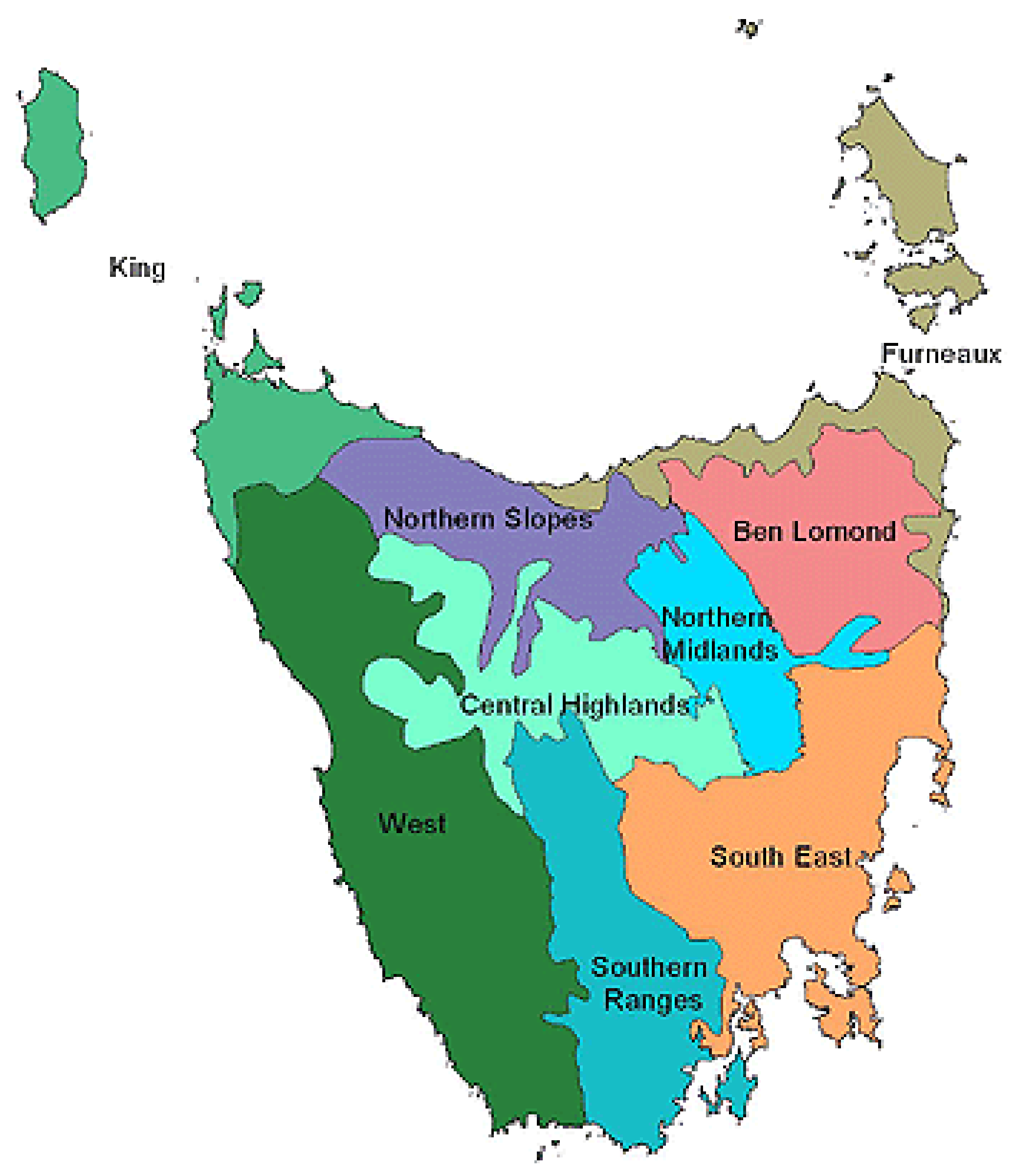
We chose Tasmania for our study due to the frequent occurrences of wildfires in the region, high-quality land data sets as maintained by Tasmania Fire Service (TFS) and State Emergency Service (SES), and a well-studied and systematic grid configuration for possible fire start locations in the region. Tasmania has a total area of 68,401 sq. km. The grid configuration for fire simulation, as maintained by TFS, places each possible fire start location at an interval of 1 sq. km irrespective of land classification. Any start locations falling on water bodies are shifted to the nearest land locations. There is a total of 68,048 possible fire start locations in the grid configuration for the entire Tasmanian region. We followed Interim Biogeographic Regionalization for Australia Version 7 (IBRA 7) [45] for nine different bio-regions (see Figure 1) to run fire simulations.
2.2. Fire Simulations—Spark
Spark [14] is a computational wildfire modeling framework that predicts the spread and potential impact of wildfires based on different behavior fire models. The framework simulates the progression of the fire over time in different fire conditions and fuels, resulting in different rates-of-spread (RoS). The fire simulations in Spark require many input data sets, including the information on land classification, fuel type, topography, and meteorological data. The simulations can be run for any number of distinct fire perimeters and can model factors such as firebreaks, spot fires, and coalescence between different parts of the fire over time. The simulations use several different empirical fire models for fuels found in Tasmania. Different fuel types found in Tasmania are mapped from the TasVeg [47] vegetation types to several empirical fire spread models. These include models for eucalypt forest [48,49], buttongrass moorland [50], heathland [51], and grasslands [52]. A detailed description of these models is included in the Appendix A.
The models require meteorological data inputs. For this study, only temperature, relative humidity, and wind speed were used [44]. Other input parameters in the fire simulation such as fuel load and land topography were used as per the configuration and records maintained by TFS and Tasmanian Government [53]. The fuel load was based on a Tasmania fire history data set allowing the time since the fire to be calculated and populated using Olson fuel load curves [54,55,56]. Our current study covered only the westerly winds as they are the most common winds in Tasmania [57,58]. The configuration and input files can be made available from the authors upon request. Based on the historical records and as considered in [5], the ranges for the data inputs are fixed as follows:
- Temperature 10–40 C
- Relative Humidity 10–90%
- Wind Speed 10–60 km/h
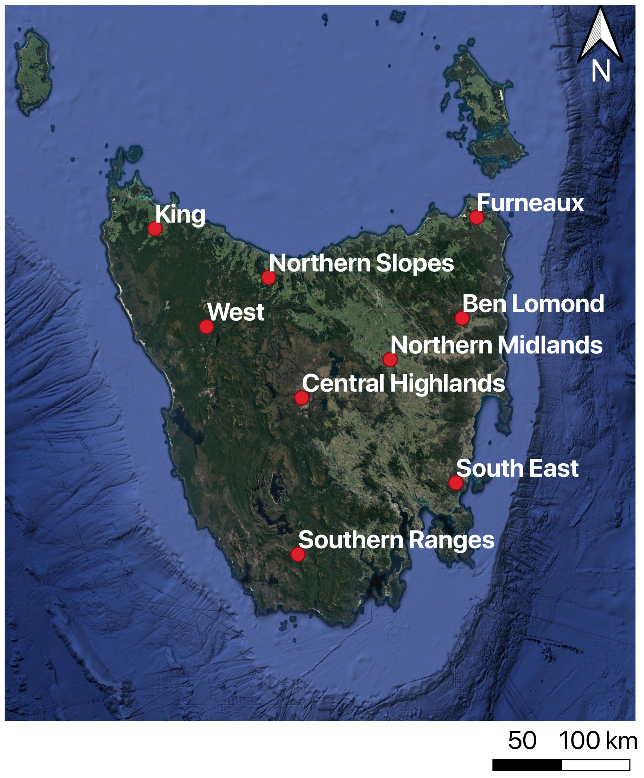
The fire simulations were started at locations in each of the nine bio-regions ensuring minimal obstructions (lakes/water bodies) irrespective of land classification locations, as shown in Figure 2. The simulations were run for a total of five hours and the area of each simulation was recorded every half-hour. The simulation data used in this study are a subset of the data available in [59].
2.3. Sensitivity Analysis
To quantify the interactions of meteorological inputs on fire dynamics, we focus on the parametric sensitivity analysis of fire simulations over time. For SA, we follow an OAT approach where the influence of a parameter is assessed by running the fire simulations for different values of the parameter within the permissible range while keeping the other parameters constant as explained in the work [60]. The influence of a parameter on the fire area is assessed by comparing the fire values obtained for the maximum and minimum values of the parameter (with minimum and maximum values of other parameters, respectively) against the fire areas obtained for the maximum (all-high) and minimum values (all-low) of all the parameters. The variability of the output of the fire simulations can be analyzed at different time steps by considering the model outputs in all these time steps to determine the scale of influence of that input parameter on the fire area. However, for our analysis to determine the cumulative influence of each parameter on the fire size, we use the total fire size obtained at the end of the total simulation time. The quantification of the variability in the fire area is carried out for each bio-region and the entirety of Tasmania as well. Similar analyses can be done to understand the influence of each parameter on the fire spread during a particular duration of time by assessing the values of the fire area.
2.4. Surrogate Modeling
For surrogate modeling of fire simulations, we first establish a mathematical model based on how fires spread over time when they ignite under some initial environmental conditions. Then, unknown values in the mathematical model are determined by fitting the simulation data by considering the results obtained from the sensitivity analysis. The mathematical relationship and simulation data fitting are discussed in detail as follows.
2.4.1. Mathematical Foundation
For a fire starting at a particular location, the shape of the fire is ideally assumed to be elliptical [61]. Consequently, the total area burnt by the fire, represented by A, is directly proportional to the square of the time (t) for which the fire is burning [61]. We focus our mathematical foundation on the same principle but replace the squared power of the time with a variable n to account for any dependency on fire geometry (ideally, the value of n in our mathematical foundation must be less than or equal to 2). As such, we mathematically express A as
where is a fitting factor that depends on the initial values of temperature (), relative humidity (), and wind speed (). This fitting factor does not account for factors such as daily temperature changes or wind changes during the progression of the fire. However, such factors are accounted for by analyzing the fire sizes for different sets (original and changed) of initial conditions and assessing the difference. The value of is determined by defining a functional form for the three input parameters based on the results of sensitivity analysis. The values of n and are determined by fitting simulation data.
2.4.2. Simulation Data Fitting
The unknown factors in Equation (1) can be determined by fitting a curve through experimental analyses. We use nonlinear least squares method [62] for data fitting. For experimental analyses, the fire simulations are run for five hours over a set of points in all nine different bio-regions in Tasmania. The simulation of fire behavior in Spark is graphically represented in Figure 3, which shows that the propagation of the fire over time can be different for different bio-regions. The steps for surrogate modeling are carried out initially for the entire Tasmanian region and then to specific bio-regions one at a time.
2.5. Surrogate Model Validation
For the validation of the dynamic model constructed in this study, we use the hold-out cross-validation method as explained in [63]. This method splits the simulation data into 70% training set and 30% test set for cross-validation. Then, to quantify the accuracy of the dynamic model, Pearson’s correlation coefficient [64] is calculated between the model predicted values and the actual values obtained from the simulations. The value of the correlation coefficient closer to one (1) represents a more accurate model.
3. Results and Discussions
3.1. Sensitivity Analysis
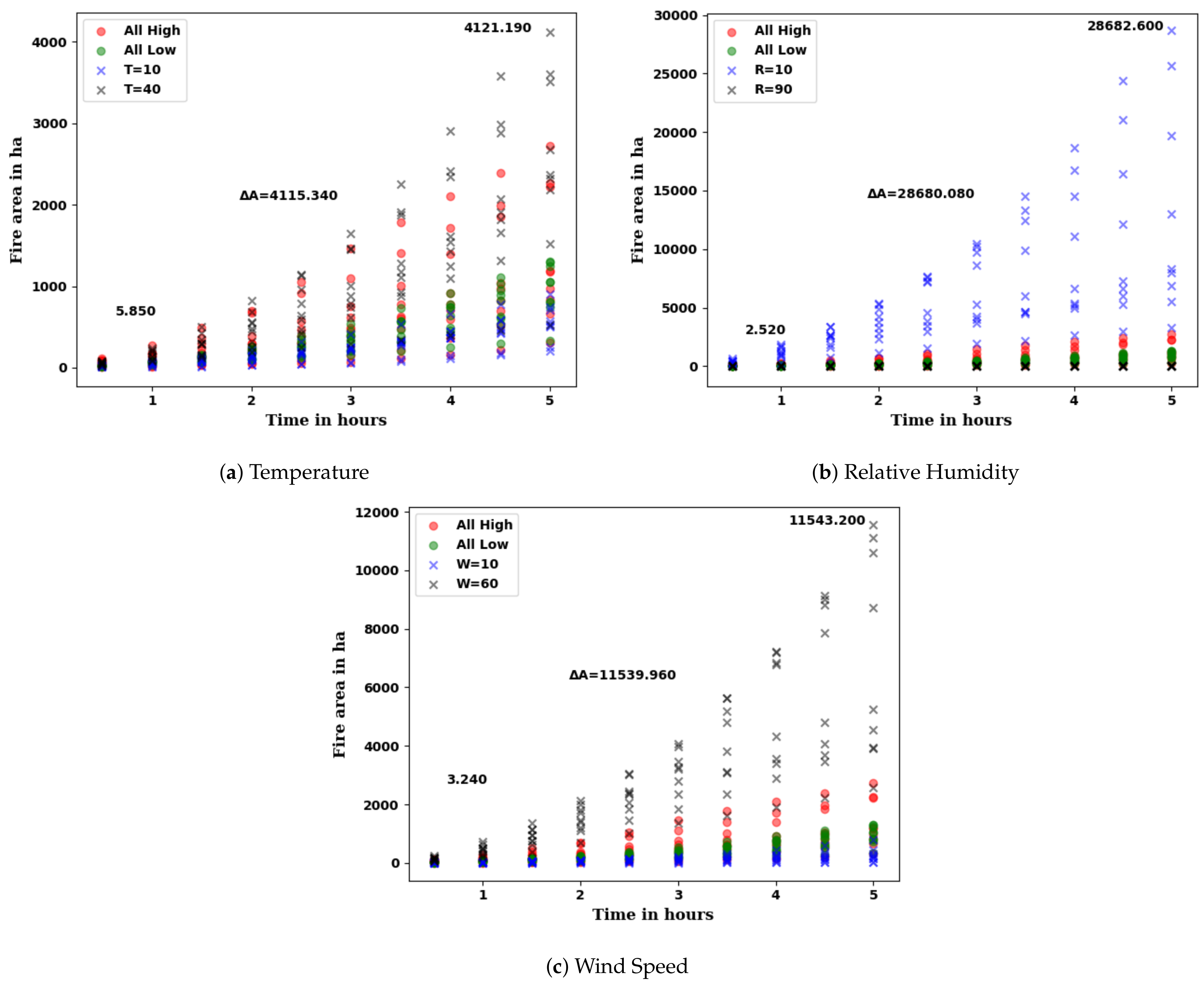
We analyzed the effect of each input parameter on the fire area size at different instants of time as given by the fire simulations in Spark run over different bio-regions in Tasmania. A plot of the variation in fire area for different bio-regions caused by variability in temperature (C) is shown in Figure 4a. The fire area generally grows bigger over time for the maximum value of the temperature. In the analysis, the fire burns a greater area at C and minimum values of other parameters. For C, the increase in the area burnt by the fire is steady until 2 h, but after that, the increase is exponential to reach a maximum value of 4121.190 ha at the five-hour mark. For a lower value of T, the increase in the fire area over time is steady and close to a linear relationship. For the entire Tasmania, the variability in burnt fire area caused by the variation of temperature is as high as 4115.340 ha. The respective variations in the fire area for different bio-regions are listed in Table 1.
The variation of the fire area with the variability of relative humidity (%) is shown in Figure 4b. It is clear from the plots that relative humidity has a significant influence on the variation of the fire area. The maximum values of the area burnt by the fire are achieved with the value of relative humidity at 10% and maximum values of other parameters for all the locations. For this particular combination of parameter values, the increase in the fire area size with time is brisk. There is a sharp increase in the rate of increase in the fire area after 2 h in general for most of the bio-regions. The maximum area burnt by fire over 5 h is 28,682.6 ha. The variation in the fire area caused by the variability of relative humidity for the entire Tasmanian region is as high as 28,680.08 ha, which is significantly higher and signifies the greater impact of the parameter. The respective variations in the fire area for different bio-regions are listed in Table 1.
The variation in the fire area caused by the variability in the wind speed (kmh) is shown in Figure 4c. The area burnt by the fire is the greatest at kmh and minimum values of other parameters for all the locations. The fire areas for other cases are relatively low. The increase in the fire area with time is steady until 2 h after which the fire area starts to increase at a higher rate. The area burnt by the fire over 5 h reaches 11,543.2 ha. The variation in the fire area caused by the variability of wind speed is approximately 11,539.96 ha for the entirety of Tasmania, which indicates the significant influence of the wind on the fire area. The respective variations in the fire area for different bio-regions are listed in Table 1.
In the analyses, we derived the upper and lower bounds for the values of the fire area for each input parameter considering the values of other parameters as well. The minimum value of an input parameter did not necessarily signify the lower bound for the fire area given by the parameter, and vice versa. For the entire Tasmanian region, the variability in fire area brought about by extreme values of temperature for extreme values of other parameters is ~4115.340 ha in five hours (see Figure 4a). The variability in fire area in the same duration caused by relative humidity is ~28,680.08 ha (see Figure 4a), while the variability caused by wind speed stands at 11,539.96 ha (see Figure 4a). As such, the extent of variability in fire area caused by relative humidity and wind speed is approximately 7 and 3 times greater than the same caused by temperature, respectively. Thus, it can be concluded that relative humidity has the highest effect on the area burnt by the fire at different instants of time for the entire Tasmanian region given by the fire simulations by Spark while the temperature has the least effect. For Northern Slopes, the variations in fire area caused by temperature and wind speed are comparable, which points out the impact caused by fuel load and land topography. Similar analyses can be done to understand the influence of each parameter on the fire spread during a particular duration of time. For example, during the second hour of a wildfire (from 1 to 2-h mark), the variation caused in the fire area by the variability in the values of temperature, relative humidity, and wind speed in the entire Tasmanian region are 739.26 ha, 5378.58 ha, and 2095.47 ha, respectively. Such information about the influence of the input parameters on the model output with consideration of the time can lead to a better quantification of the feedback of meteorological inputs on the fire dynamics.
We used an OAT method to measure the influence of each input parameter on the output of the fire simulations. To understand the variation in fire area in different bio-regions, we carried out the analyses for all the regions independently. In our analyses, we derived the upper and lower bounds for the values of the fire area for each input parameter considering the values of other parameters as well. For all the bio-regions, the variation in the fire area caused by the variability of relative humidity is the highest, while the variation caused by that of the temperature is the lowest. The variations in fire area caused by the variability of relative humidity and wind speed are as high as about 11 and 5 times more when compared to the same caused by the variability of temperature, respectively. For Northern Slopes, the variations in fire area caused by temperature and wind speed are comparable, which points out the impact caused by fuel load and land topography. The quantitative measure of the variability in fire area brought by each parameter during the OAT method is conclusive. Our findings established relative humidity as the parameter with the greatest impact on the spread of the fire over time and temperature as the one with the least impact. This finding can be attributed to the fire models in Spark that are highly sensitive to fuel moisture content, which in turn is highly sensitive to relative humidity compared to temperature (for example, the Dry Eucalypt model equation for fuel moisture content, , has a greater dependency on relative humidity than temperature). However, the extent of the influence of each parameter on the variability of the fire area size is not necessarily the same for all the bio-regions even though they have similar relative comparisons.
3.2. Surrogate Modeling
Following the methods defined for surrogate modeling (Equation (1)), we first incorporated the meteorological influence and adapted a functional form for temperature, relative humidity, and wind speed to determine the value of . The functional form was developed by further analyzing the results of the sensitivity analysis in which the growth of fire area was investigated at different time instants (every half-hour mark) against the highest values of the input parameters (Figure 5). As can be seen in the figure, the growth of the fire area is close to linear over time for temperature and relative humidity, whereas an exponential fit is more suitable for wind speed. As such, the functional form for input parameter to define the factor in our surrogate model (Equation (1)) is
After fitting the simulation data obtained from all the Tasmanian regions, the surrogate model is defined as follows:
Note that the functional form used for the surrogate model is slightly different from the formulation in the work of Sharples et al. [44] as the surrogate model is based on the findings from the uncertainty quantification.
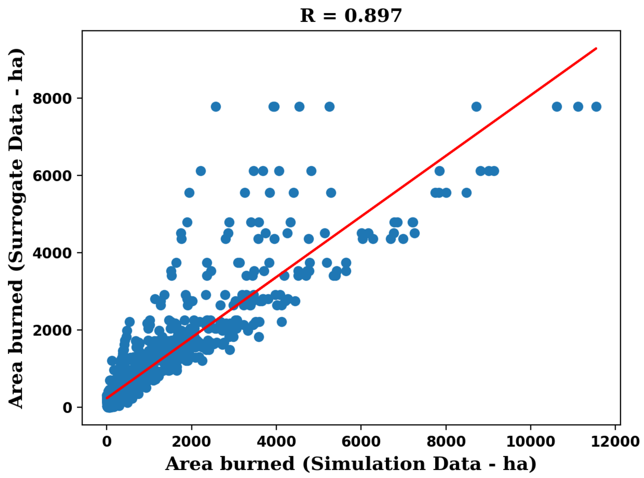
The simulation and predicted data are shown in Figure 6. The value of the correlation coefficient is 0.897. Interestingly, the value of power to which the time is raised in the model is close to 2 (1.76), indicating fire growth scales approximately as the expected square of the time. Despite the high value of the correlation coefficient, the model over fits the fire area for some extreme values of the input parameters. Although not ideal, an overfitted result produces a more conservative estimate of larger fire sizes, rather than a possibly dangerous underestimate. The overfitting in the model is possibly due to the significant impact of the fuel loads, which can be different for different bio-regions, and the interaction between the input parameters, which are not considered in the study. The fitting parameters for each individual region in Tasmania are given in Table 2 and plotted in Figure 7.
Our surrogate model based on fire simulations has reasonable success with promising findings. The mathematical equation defined in the surrogate model in terms of the initial values of different meteorological data gave satisfactory information about the progression of the fire over time as the value of the calculated correlation coefficient for the entire Tasmanian region is about 0.897. This finding indicates the fact that constructing a surrogate model to represent all the bio-regions with a diverse range of fuel loads and land topography may not be so efficient. Consequently, we constructed a single surrogate model for each bio-region and calculated the correlation coefficient between the simulation data and the model predicted data, as shown in Figure 7. Moreover, as listed in Table 2, the values of unknown parameters also represent the respective influence of the parameters in the forest area burnt by the fire. The findings of the surrogate models are consistent with the results obtained from our sensitivity analysis carried out by considering different instants of time. The negative values of indicate that the fire grows rapidly under lower values of relative humidity when compared to the higher values, while the higher values of reflect the strong influence of relative humidity on the fire area. The negative value of as determined in our study is quite consistent with the functional form defined by Shaples et al. in [44] for spread index, where the relative humidity in the denominator indicates a higher spread rate (consequently higher fire area) at lower values when compared to the same at higher values. Further, the surrogate model constructed to represent the dynamics of fire in terms of initial environmental conditions closely represents the actual behavior of the fire over time as the values of the correlation coefficient are well over 0.987. The surrogate model incorrectly identifies small fires, possibly due to the presence of a lake or other water bodies near the fire start location. However, the model shows a good match for larger fires in most cases. This is useful for operational fire management, as recent studies have shown the opposite trend for fire simulations [65], where fire predictions using forecast weather in fire simulation tools under-predicted the fire size in extreme weather conditions. Considering other location-specific information in the model can improve the closeness of the model estimation with the actual values. For the Southern Ranges bio-region, the model has a correlation coefficient of 0.996, which signifies the fact that the model closely matches the fire dynamics from the simulations in the region. Such a good prediction by the model appears to be due to the region being relatively free of obstructions (lakes/built-up areas) where the fire would otherwise be stopped. This finding indicates that surrogate models, like the one built here in the study, can be helpful for quickly estimating fires under extreme fire weather conditions for large open areas. The lowest value of the correlation coefficient for the model is 0.910 in the Northern Slopes region, which is likely due to the presence of wetlands in the region and due to nonlinear interactions between the input parameters. The nonlinear interactions between the input parameters are not considered for this study. This particular aspect of the surrogate model will be strengthened in the future to improve the closeness of the data predicted by the model with the actual simulation data.
The constructed surrogate model can represent the change in the size of the fire with time-based on the initial values of meteorological inputs (temperature, relative humidity, and wind speed). This could be used to rapidly estimate the wildfire risks, although it should be emphasized that the model can only give an estimate of the size of the fire rather than the shape, growth, or possible impact on certain areas. The functional form to estimate the fire size obtained in this study can be an alternative form to the one explained in [44]. Additionally, our attempt to investigate the path of fire growth has shown that in practical scenarios, the fire area does not follow an ideal relationship as the values of n as obtained in our experimental analyses for all nine bio-regions are less than 2.
4. Conclusions and Future Works
In this paper, we analyzed the contribution of different parameters on the area (geographical extent) burnt by the fire over time in a conventional one-at-a-time (OAT) fashion by considering nine different bio-regions in Tasmania. Relative Humidity was found to be the parameter with the greatest impact on the spread of fire over time, while Temperature was found to have the least effect. Moreover, our analyses were time-dependent, allowing new ways to quantify the feedback of meteorological inputs on the fire dynamics, and vice versa. Information about the sensitivity of parameters in wildfire models could facilitate new operational approaches for risk management by excluding less sensitive parameters from the models allowing risk to be calculated in a shorter time-frame. We used simulations to construct a computationally-efficient surrogate model for the area of a fire over time in terms of initial starting conditions. The surrogate model considered the nature and the extent of the influence of each meteorological input on the fire dynamics. The region-specific surrogate models constructed in this study represented the dynamic fire behaviors except for some extreme cases. Such surrogate models may be helpful in operational wildfire management during emergencies to quickly make informed decisions for response activities by providing a rapid estimate of potential fire size.
This study is one of the preliminary works to explore sensitivity analyses at different instants of time and how results of such analyses can be integrated into natural hazard modeling systems. In the future, we will take the nonlinear interactions between the input parameters into account to strengthen the surrogate model. The study can be extended for other regions as well with sufficient fire simulation data in hand.
Author Contributions
Conceptualization, U.K. and J.A.; Formal analysis, U.K.; Investigation, U.K.; Methodology, U.K. and J.A.; Software, J.H.; Supervision, J.A., J.H. and S.G.; Validation, U.K. and J.H.; Visualization, U.K.; Writing—original draft, U.K. and J.H.; Writing—review and editing, U.K., J.A., J.H., and S.G. All authors have read and agreed to the published version of the manuscript.
Funding
This research received no external funding.
Institutional Review Board Statement
Not applicable.
Informed Consent Statement
Not applicable.
Data Availability Statement
Not applicable.
Acknowledgments
The authors would like to thank our academic colleagues who helped in improving the quality of the manuscript at various stages of the work.
Conflicts of Interest
The authors declare no conflict of interest.
Appendix A
Appendix A.1. McArthur Grassland Fire Danger Meters
McArthur [48] described his research into grassland fire behavior in terms of the Grassland Fire Danger Index (GFDI), based on which the rate of spread was calculated. The equations for GFDI and rate of spread (R) are listed as follows:
C is the degree of curing (%), T is the air temperature (), is the relative humidity (%), and is the wind speed (km/h) measured at a height of 10-m in the open.
R is the headfire rate of spread (km/h).
Appendix A.2. Dry Eucalypt Model (Cheney et al.)
This wildfire model is used for predicting the spread of fire behaviors in dry eucalypt forest. The model was developed from a sequence of experiments called “project Vesta” [49] carried out in south-western Australia. The mathematical equations for the model are listed as follows:
Note that the term is the model correction for bias and is taken as 1.03 for this. is the near-surface fuel hazard score, is the surface fuel hazard score, and is near-surface height and are derived from fuel age using the tall shrubs regression equations as explained in [66].
R is the rate of spread (m/h), is the average 10-m open wind speed (km/h), and is the fuel moisture function.
T is the air temperature () and is the relative humidity (%).
Appendix A.3. CSIRO Grassland Model
Based on the experimental results obtained from the burning project in the Northern Territory of Australia, Cheney et al. [52] described a relationship for the rate of fire spread on grasslands. This model was developed to settle down the confusion created after the calculation of different Grassland Fire Danger Index (GFDI) values under the same conditions thereby questioning the actual effect of fuel load on fire spread rate. The mathematical equations in the model are explained as follows:
is the cut/grazed rate of spreed in m/s, is the 10-m open wind speed (km/h), is the fuel moisture coefficient, and is the curing coefficient.
is the dead fuel moisture content (% oven-dry weight basis).
T is the temperature (C and is the relative humidity (%).
C is the degree of grass curing (%).
Note that the original equation for proposed by Cheney et al. was modified by Cruz et al. as the curing level can be as low as 20% and the damping effects of the fuel in grassland is less.
Appendix A.4. Marsden–Smedley and Catchpole Buttongrass Model
Marsden–Smedly and Catchpole [50] described the fire behaviors for buttongrass moorlands in Tasmania for fire danger rating and fire behavior prediction. The mathematical equations for the models are explained as follows:
where is the wind speed (km/h) measured at a 2-m height, is the dead fuel moisture content (%), and is the time since the last fire (years).
is the dew point temperature () and is the relative humidity (%).
Appendix A.5. Anderson et al. Heathland Model
Anderson et al. [51] used a dataset that covered a wider range of heathland and shrubland species to develop a model for healthland as an extension to the work [69]. The equations for the model are given as follows:
where R is the rate of spread (m/min) with vegetation height and without live fuel moisture content, is the 10-m open wind speed (km/h), H is the average vegetation height (m), is the wind adjustment factor, and is the dead fuel moisture content (%).
for sunny days from 12:00 to 17:00 from October to March and 0 elsewhere. T is the ambient air temperature (C and is the relative humidity (%).
References
- National Inter-Agency Fire Center. Available online: https://www.nifc.gov/fireInfo/fireInfo_statistics.html (accessed on 12 May 2019).
- Munich RE. Available online: https://www.munichre.com/australia/australia-natural-hazards/bushfires/economic-impacts/index.html (accessed on 12 May 2019).
- North, M.; Stephens, S.; Collins, B.; Agee, J.; Aplet, G.; Franklin, J.; Fule, P.Z. Reform forest fire management. Science 2015, 349, 1280–1281. [Google Scholar] [CrossRef] [PubMed]
- Whelan, R.J. The Ecology of Fire; Cambridge University Press: Cambridge, UK, 1995. [Google Scholar]
- Ujjwal, K.; Garg, S.; Hilton, J.; Aryal, J. A cloud-based framework for sensitivity analysis of natural hazard models. Environ. Model. Softw. 2020, 134, 104800. [Google Scholar]
- Sullivan, A.L. Wildland surface fire spread modelling, 1990–2007. 3: Simulation and mathematical analogue models. Int. J. Wildland Fire 2009, 18, 387–403. [Google Scholar] [CrossRef] [Green Version]
- Grishin, A. Mathematical Modeling of Forest Fires and New Methods of Fighting Them, edited by FA Albini Publishing House of the Tomsk University. Tomsk. Russ. 1997, 29, 917–919. [Google Scholar]
- Mell, W.; Jenkins, M.A.; Gould, J.; Cheney, P. A physics-based approach to modelling grassland fires. Int. J. Wildland Fire 2007, 16, 1–22. [Google Scholar] [CrossRef]
- Morvan, D. Physical phenomena and length scales governing the behaviour of wildfires: a case for physical modelling. Fire Technol. 2011, 47, 437–460. [Google Scholar] [CrossRef]
- Morvan, D.; Dupuy, J. Modeling the propagation of a wildfire through a Mediterranean shrub using a multiphase formulation. Combust. Flame 2004, 138, 199–210. [Google Scholar] [CrossRef]
- Gould, J.S.; McCaw, W.; Cheney, N.; Ellis, P.; Knight, I.; Sullivan, A. Project Vesta: Fire in Dry Eucalypt Forest: Fuel Structure, Fuel Dynamics and Fire Behaviour; Csiro Publishing: Collingwood, Australia, 2008. [Google Scholar]
- Tanskanen, H.; Granström, A.; Larjavaara, M.; Puttonen, P. Experimental fire behaviour in managed Pinus sylvestris and Picea abies stands of Finland. Int. J. Wildland Fire 2007, 16, 414–425. [Google Scholar] [CrossRef]
- Baeza, M.; De Luıs, M.; Raventós, J.; Escarré, A. Factors influencing fire behaviour in shrublands of different stand ages and the implications for using prescribed burning to reduce wildfire risk. J. Environ. Manag. 2002, 65, 199–208. [Google Scholar] [CrossRef] [PubMed]
- Miller, C.; Hilton, J.; Sullivan, A.; Prakash, M. SPARK—A bushfire spread prediction tool. In Proceedings of the International Symposium on Environmental Software Systems, Melbourne, VIC, Australia, 25–27 March 2015; Springer: Berlin/Heidelberg, Germany, 2015; pp. 262–271. [Google Scholar]
- Finney, M.A. FARSITE: Fire Area Simulator-model development and evaluation. In Res. Pap. RMRS-RP-4, Revised 2004. Ogden, UT; US Department of Agriculture, Forest Service, Rocky Mountain Research Station: Fort Collins, CO, USA, 1998; Volume 4, 47p. [Google Scholar]
- Rothermel, R.C. A mathematical model for predicting fire spread in wildland fuels. In Res. Pap. INT-115; US Department of Agriculture, Intermountain Forest and Range Experiment Station: Ogden, UT, USA, 1972; Volume 115, 40p. [Google Scholar]
- Vakalis, D.; Sarimveis, H.; Kiranoudis, C.; Alexandridis, A.; Bafas, G. A GIS based operational system for wildland fire crisis management I. Mathematical modelling and simulation. Appl. Math. Model. 2004, 28, 389–410. [Google Scholar] [CrossRef]
- Nahmias, J.; Téphany, H.; Duarte, J.; Letaconnoux, S. Fire spreading experiments on heterogeneous fuel beds. Applications of percolation theory. Can. J. For. Res. 2000, 30, 1318–1328. [Google Scholar] [CrossRef]
- Méndez, V.; Llebot, J.E. Hyperbolic reaction-diffusion equations for a forest fire model. Phys. Rev. E 1997, 56, 6557. [Google Scholar] [CrossRef] [Green Version]
- Noble, I.; Gill, A.; Bary, G. McArthur’s fire-danger meters expressed as equations. Aust. J. Ecol. 1980, 5, 201–203. [Google Scholar] [CrossRef]
- Trucchia, A.; Egorova, V.; Pagnini, G.; Rochoux, M.C. On the merits of sparse surrogates for global sensitivity analysis of multi-scale nonlinear problems: Application to turbulence and fire-spotting model in wildland fire simulators. Commun. Nonlinear Sci. Numer. Simul. 2019, 73, 120–145. [Google Scholar] [CrossRef] [Green Version]
- Hilton, J.E.; Stephenson, A.G.; Huston, C.; Swedosh, W. Polynomial Chaos for sensitivity analysis in wildfire modelling. In Proceedings of the International Congress on Modelling and Simulation, Hobart, Australia, 3–8 December 2017. [Google Scholar]
- Tolhurst, K.; Shields, B.; Chong, D. Phoenix: development and application of a bushfire risk management tool. Aust. J. Emerg. Manag. 2008, 23, 47. [Google Scholar]
- Ujjwal, K.; Garg, S.; Hilton, J. An efficient framework for ensemble of natural disaster simulations as a service. Geosci. Front. 2020, 11, 1859–1873. [Google Scholar]
- Riley, K.; Thompson, M.; Riley, K.; Webley, P.; Thompson, M. An uncertainty analysis of wildfire modeling. Nat. Hazard Uncertain. Assess. Model. Decis. Support. Monogr. 2017, 223, 193–213. [Google Scholar]
- Kaschek, D.; Mader, W.; Fehling-Kaschek, M.; Rosenblatt, M.; Timmer, J. Dynamic modeling, parameter estimation and uncertainty analysis in R. bioRxiv 2016, 085001. [Google Scholar] [CrossRef] [Green Version]
- Nossent, J.; Elsen, P.; Bauwens, W. Sobol’sensitivity analysis of a complex environmental model. Environ. Model. Softw. 2011, 26, 1515–1525. [Google Scholar] [CrossRef]
- Saltelli, A.; Ratto, M.; Andres, T.; Campolongo, F.; Cariboni, J.; Gatelli, D.; Saisana, M.; Tarantola, S. Global Sensitivity Analysis: The Primer; John Wiley & Sons: Hoboken, NJ, USA, 2008. [Google Scholar]
- Cai, L.; He, H.S.; Liang, Y.; Wu, Z.; Huang, C. Analysis of the uncertainty of fuel model parameters in wildland fire modelling of a boreal forest in north-east China. Int. J. Wildland Fire 2019, 28, 205–215. [Google Scholar] [CrossRef]
- Brohus, H.; Nielsen, P.V.; Petersen, A.J.; Sommerlund-Larsen, K. Sensitivity analysis of fire dynamics simulation. In Proceedings of the Roomvent 2007, Helsinki, Finland, 13–15 June 2007. [Google Scholar]
- Salvador, R.; Pinol, J.; Tarantola, S.; Pla, E. Global sensitivity analysis and scale effects of a fire propagation model used over Mediterranean shrublands. Ecol. Model. 2001, 136, 175–189. [Google Scholar] [CrossRef]
- Li, X.; Hadjisophocleous, G.; Sun, X.Q. Sensitivity and Uncertainty Analysis of a Fire Spread Model with Correlated Inputs. Procedia Eng. 2018, 211, 403–414. [Google Scholar] [CrossRef]
- Yuan, X.; Liu, N.; Xie, X.; Viegas, D.X. Physical model of wildland fire spread: Parametric uncertainty analysis. Combust. Flame 2020, 217, 285–293. [Google Scholar] [CrossRef]
- Marcot, B.G.; Thompson, M.P.; Runge, M.C.; Thompson, F.R.; McNulty, S.; Cleaves, D.; Tomosy, M.; Fisher, L.A.; Bliss, A. Recent advances in applying decision science to managing national forests. For. Ecol. Manag. 2012, 285, 123–132. [Google Scholar] [CrossRef]
- Ujjwal, K.; Garg, S.; Hilton, J.; Aryal, J.; Forbes-Smith, N. Cloud Computing in natural hazard modeling systems: Current research trends and future directions. Int. J. Disaster Risk Reduct. 2019, 38, 101188. [Google Scholar]
- Bass, B.; Bedient, P. Surrogate modeling of joint flood risk across coastal watersheds. J. Hydrol. 2018, 558, 159–173. [Google Scholar] [CrossRef]
- Bermúdez, M.; Ntegeka, V.; Wolfs, V.; Willems, P. Development and comparison of two fast surrogate models for urban pluvial flood simulations. Water Resour. Manag. 2018, 32, 2801–2815. [Google Scholar] [CrossRef]
- Kim, S.W.; Melby, J.A.; Nadal-Caraballo, N.C.; Ratcliff, J. A time-dependent surrogate model for storm surge prediction based on an artificial neural network using high-fidelity synthetic hurricane modeling. Nat. Hazards 2015, 76, 565–585. [Google Scholar] [CrossRef]
- Jia, G.; Taflanidis, A.A. Kriging metamodeling for approximation of high-dimensional wave and surge responses in real-time storm/hurricane risk assessment. Comput. Methods Appl. Mech. Eng. 2013, 261, 24–38. [Google Scholar] [CrossRef]
- Easum, J.A.; Nagar, J.; Werner, P.L.; Werner, D.H. Efficient multiobjective antenna optimization with tolerance analysis through the use of surrogate models. IEEE Trans. Antennas Propag. 2018, 66, 6706–6715. [Google Scholar] [CrossRef]
- Sanchez, F.; Budinger, M.; Hazyuk, I. Dimensional analysis and surrogate models for the thermal modeling of Multiphysics systems. Appl. Therm. Eng. 2017, 110, 758–771. [Google Scholar] [CrossRef] [Green Version]
- Meng, D.; Yang, S.; Zhang, Y.; Zhu, S.P. Structural reliability analysis and uncertainties-based collaborative design and optimization of turbine blades using surrogate model. Fatigue Fract. Eng. Mater. Struct. 2019, 42, 1219–1227. [Google Scholar] [CrossRef]
- Ökten, G.; Liu, Y. Randomized quasi-Monte Carlo methods in global sensitivity analysis. Reliab. Eng. Syst. Saf. 2021, 210, 107520. [Google Scholar] [CrossRef]
- Sharples, J.J.; Bahri, M.F.; Huntley, S. A universal rate of spread index for Australian fuel types. In Proceedings of the International Conference on Forest Fire Research, Coimbra, Portugal, 10–16 November 2018; Available online: https://www.environment.gov.au/system/files/pages/5b3d2d31-2355-4b60-820c-e370572b2520/files/bioregions-new.pdf (accessed on 12 March 2020).
- IBRA7. Available online: http://www.environment.gov.au/system/files/pages/5b3d2d31-2355-4b60-820c-e370572b2520/files/bioregions-new.pdf (accessed on 12 March 2020).
- Tasmania’s Bioregions. Available online: https://dpipwe.tas.gov.au/conservation/flora-of-tasmania/tasmanias-wetlands (accessed on 12 April 2021).
- Tasmanian Department of Primary Industries, Parks, W.; Monitoring, E.T.V.; Program, M. TasVeg 3.0. 2013. Available online: https://www.threatenedspecieslink.tas.gov.au/Pages/tasveg-3.aspx (accessed on 12 December 2020).
- McArthur, A.G. Fire Behaviour in Eucalypt Forests Forestry and Timber Bureau. Canberra, 1967. Available online: https://catalogue.nla.gov.au/Record/2275488 (accessed on 12 March 2021).
- Cheney, N.P.; Gould, J.S.; McCaw, W.L.; Anderson, W.R. Predicting fire behaviour in dry eucalypt forest in southern Australia. For. Ecol. Manag. 2012, 280, 120–131. [Google Scholar] [CrossRef]
- Marsden-Smedley, J.; Catchpole, W.R. Fire behaviour modelling in Tasmanian buttongrass moorlands. II. Fire behaviour. Int. J. Wildland Fire 1995, 5, 215–228. [Google Scholar] [CrossRef]
- Anderson, W.R.; Cruz, M.G.; Fernandes, P.M.; McCaw, L.; Vega, J.A.; Bradstock, R.A.; Fogarty, L.; Gould, J.; McCarthy, G.; Marsden-Smedley, J.B.; et al. A generic, empirical-based model for predicting rate of fire spread in shrublands. Int. J. Wildland Fire 2015, 24, 443–460. [Google Scholar] [CrossRef] [Green Version]
- Cheney, N.; Gould, J.; Catchpole, W.R. Prediction of fire spread in grasslands. Int. J. Wildland Fire 1998, 8, 1–13. [Google Scholar] [CrossRef]
- List Data. Available online: https://listdata.thelist.tas.gov.au/opendata/ (accessed on 12 March 2021).
- Olson, J.S. Energy storage and the balance of producers and decomposers in ecological systems. Ecology 1963, 44, 322–331. [Google Scholar] [CrossRef] [Green Version]
- Birk, E.M.; Simpson, R. Steady state and the continuous input model of litter accumulation and decompostion in Australian eucalypt forests. Ecology 1980, 61, 481–485. [Google Scholar] [CrossRef]
- Fire Prediction Services. PHOENIXRapidFire: Technical Reference Guide; A Technical Guide to the PHOENIX RapidFire Bushfire Characterisation ModelVersion 4; Australasian Fire and Emergency Service Authorities Council: Melbourne, VIC, Australia, 2019; Volume 1.
- Abatzoglou, J.T.; Hatchett, B.J.; Fox-Hughes, P.; Gershunov, A.; Nauslar, N.J. Global climatology of synoptically-forced downslope winds. Int. J. Climatol. 2021, 41, 31–50. [Google Scholar] [CrossRef]
- Fox-Hughes, P. A fire danger climatology for Tasmania. Aust. Meteorol. Mag. 2008, 57, 109–120. [Google Scholar]
- KC, U.; Garg, S.; Hilton, J.; Aryal, J. Fire Simulation Data Set for Tasmania; CSIRO: Hobart, Australia; University of Tasmania: Hobart, Australia, 2021. [Google Scholar] [CrossRef]
- Hamby, D. A review of techniques for parameter sensitivity analysis of environmental models. Environ. Monit. Assess. 1994, 32, 135–154. [Google Scholar] [CrossRef] [PubMed]
- Wagner, C.V. A simple fire-growth model. For. Chron. 1969, 45, 103–104. [Google Scholar] [CrossRef] [Green Version]
- Levenberg, K. A method for the solution of certain non-linear problems in least squares. Q. Appl. Math. 1944, 2, 164–168. [Google Scholar] [CrossRef] [Green Version]
- Kohavi, R. A study of cross-validation and bootstrap for accuracy estimation and model selection. InIjcai 1995, 14, 1137–1145. [Google Scholar]
- Benesty, J.; Chen, J.; Huang, Y.; Cohen, I. Pearson correlation coefficient. In Noise Reduction in Speech Processing; Springer: Berlin/Heidelberg, Germany, 2009; pp. 1–4. [Google Scholar]
- Penman, T.D.; Ababei, D.A.; Cawson, J.G.; Cirulis, B.A.; Duff, T.J.; Swedosh, W.; Hilton, J.E. Effect of weather forecast errors on fire growth model projections. Int. J. Wildland Fire 2020, 29, 983–994. [Google Scholar] [CrossRef]
- Gould, J.S.; McCaw, W.L.; Cheney, N.P. Quantifying fine fuel dynamics and structure in dry eucalypt forest (Eucalyptus marginata) in Western Australia for fire management. For. Ecol. Manag. 2011, 262, 531–546. [Google Scholar] [CrossRef]
- Gould, J.S.; McCaw, W.; Cheney, N.; Ellis, P.; Matthews, S. Field Guide: Fire in Dry Eucalypt Forest: Fuel Assessment and Fire Behaviour Prediction in Dry Eucalypt Forest; CSIRO Publishing: Collingwood, Australia, 2008. [Google Scholar]
- Matthews, S.; Gould, J.; McCaw, L. Simple models for predicting dead fuel moisture in eucalyptus forests. Int. J. Wildland Fire 2010, 19, 459–467. [Google Scholar] [CrossRef]
- Catchpole, W.; Bradstock, R.; Choate, J.; Fogarty, L.; Gellie, N.; McCarthy, G.; McCaw, W.; Marsden-Smedley, J.; Pearce, G. Cooperative development of equations for heathland fire behaviour. In Proceedings of the 3rd International Conference on Forest Fire Research and 14th Conference on Fire and Forest Meteorology, Coimbra, Portugal, 16–20 November 1998; Volume 2, pp. 16–20. [Google Scholar]
Figure 1.
Nine bio-regions of Tasmania. Sourced from the work in [46].
Figure 1.
Nine bio-regions of Tasmania. Sourced from the work in [46].

Figure 2.
Fire start locations for different bio-regions in Tasmania. The locations are chosen ensuring minimal obstructions due to water bodies irrespective of land classification.
Figure 2.
Fire start locations for different bio-regions in Tasmania. The locations are chosen ensuring minimal obstructions due to water bodies irrespective of land classification.

Figure 3.
Illustration of simulation in Fire dynamics in Spark (). The wildfire propagates differently based on the fuel load and land topography and consequently, the total area burnt by the fire varies based on the bio-region. Different colors represent the area burnt by the fire over time in half hourly steps. The purple color represents the area burnt by the fire in the first half hour, while the red color represents the area burnt from 4.5–5 h mark.

Figure 4.
Variation of fire area (in ) with the variability of different input parameters, shown as on the plots. All high is the plot for fire area obtained with maximum values of all parameters, while all low is with minimum values. The variation of fire area caused by relative humidity is the highest while that of the temperature is the lowest.

Figure 5.
Rate of increase of fire area with time for Southern Ranges bio-region (The rate of increase in the fire area is in hectares per minute (ha ). The contributions in the rate of change of fire area made by temperature (blue line) and relative humidity (red) are steady over time while the same made by the wind speed (green) increases exponentially over time).

Figure 6.
Simulation Data vs. model predicted data for entire Tasmania (The area burnt by the fire is in hectares (). The red line represents the ideal line where the scatter plots should align for the most accurate surrogate prediction data. The calculated value of correlation coefficient is 0.897, which indicates that the surrogate model closely predicted the actual simulation data.)

Figure 7.
Bio-region-specific surrogate model predicted data compared against simulation data. The fire area is in hectares (). The red line represents the ideal line where the scatter plots should align for the most accurate surrogate prediction data. The surrogate model constructed for the Southern Ranges bio-region has the highest value of correlation coefficient of 0.996 while that of Northern Slopes is the lowest with a value of 0.910.


Table 1.
Variability in fire area caused by variability in input parameters.
| Bio-Regions | Variation in Area burnt by fire () in | ||
|---|---|---|---|
| Temperature | Rel. Humidity | Wind | |
| Southern Ranges | 2655.18 | 28,679.9 | 11,531.23 |
| South East | 2360.97 | 25,645.92 | 11,114.86 |
| West | 1143.36 | 3308.58 | 2554.11 |
| Central Highlands | 2290.32 | 8328.78 | 4524.47 |
| Northern Slopes | 4092.21 | 5543.11 | 3910.05 |
| Northern Midlands | 2177.55 | 7995.96 | 5239.71 |
| Ben Lomond | 3573.72 | 19,713.78 | 10,601.4 |
| Furneaux | 3491.91 | 12,972.73 | 8702.5 |
| King | 1497.33 | 6908.67 | 3943.89 |
| Tasmania | 4115.34 | 28,680.08 | 11,539.96 |
Table 2.
Fitting parameters in the surrogate model for nine bio-regions in Tasmania.
| Bio-Regions | n | |||
|---|---|---|---|---|
| Southern Ranges | 17.26 | −41.98 | 2.09 | 1.91 |
| South East | 35.56 | −137.33 | 2.38 | 1.81 |
| West | 2.49 | −5.56 | 1.46 | 1.49 |
| Central Highlands | 14.95 | −16.54 | 1.87 | 1.76 |
| Northern Slopes | 12.11 | −39.69 | 2.21 | 1.68 |
| Northern Midlands | 30.38 | −19.13 | 1.95 | 1.72 |
| Ben Lomond | 23.09 | −35.29 | 2.34 | 1.81 |
| Furneaux | 26.09 | −53.85 | 2.43 | 1.73 |
| King | 11.21 | −9.80 | 1.78 | 1.60 |
| Tasmania | 16.72 | −26.80 | 2.03 | 1.76 |
Publisher’s Note: MDPI stays neutral with regard to jurisdictional claims in published maps and institutional affiliations. |
© 2021 by the authors. Licensee MDPI, Basel, Switzerland. This article is an open access article distributed under the terms and conditions of the Creative Commons Attribution (CC BY) license (https://creativecommons.org/licenses/by/4.0/).
Share and Cite
MDPI and ACS Style
KC, U.; Aryal, J.; Hilton, J.; Garg, S. A Surrogate Model for Rapidly Assessing the Size of a Wildfire over Time. Fire 2021, 4, 20. https://0-doi-org.brum.beds.ac.uk/10.3390/fire4020020
AMA Style
KC U, Aryal J, Hilton J, Garg S. A Surrogate Model for Rapidly Assessing the Size of a Wildfire over Time. Fire. 2021; 4(2):20. https://0-doi-org.brum.beds.ac.uk/10.3390/fire4020020
Chicago/Turabian StyleKC, Ujjwal, Jagannath Aryal, James Hilton, and Saurabh Garg. 2021. "A Surrogate Model for Rapidly Assessing the Size of a Wildfire over Time" Fire 4, no. 2: 20. https://0-doi-org.brum.beds.ac.uk/10.3390/fire4020020