Continuous Evaluation of Track Modulus from a Moving Railcar Using ANN-Based Techniques


Department of Civil & Environmental Engineering, University of Alberta, Edmonton, AB T6G 1H9, Canada
*
Author to whom correspondence should be addressed.
Vibration 2020, 3(2), 149-161; https://0-doi-org.brum.beds.ac.uk/10.3390/vibration3020012
Submission received: 12 May 2020
/
Revised: 17 June 2020
/
Accepted: 18 June 2020
/
Published: 22 June 2020
(This article belongs to the Special Issue Inverse Dynamics Problems)
Abstract
:Track foundation stiffness (also referred as the track modulus) is one of the main parameters that affect the track performance, and thus, quantifying its magnitudes and variations along the track is widely accepted as a method for evaluating the track condition. In recent decades, the train-mounted vertical track deflection measurement system developed at the University of Nebraska–Lincoln (known as the MRail system) appears as a promising tool to assess track structures over long distances. Numerical methods with different levels of complexity have been proposed to simulate the MRail deflection measurements. These simulations facilitated the investigation and quantification of the relationship between the vertical deflections and the track modulus. In our previous study, finite element models (FEMs) with a stochastically varying track modulus were used for the simulation of the deflection measurements, and the relationships between the statistical properties of the track modulus and deflections were quantified over different track section lengths using curve-fitting approaches. The shortcoming is that decreasing the track section length resulted in a lower accuracy of estimations. In this study, the datasets from the same FEMs are used for the investigations, and the relationship between the measured deflection and track modulus averages and standard deviations are quantified using artificial neural networks (ANNs). Different approaches available for training the ANNs using FEM datasets are discussed. It is shown that the estimation accuracy can be significantly increased by using ANNs, especially when the estimations of track modulus and its variations are required over short track section lengths, ANNs result in more accurate estimations compared to the use of equations from curve-fitting approaches. Results also show that ANNs are effective for the estimations of track modulus even when the noisy datasets are used for training the ANNs.
1. Introduction
It is widely accepted that a track modulus, and its variations, are indicators of subgrade conditions [1,2,3,4,5]. A track modulus is a measure of the vertical stiffness of the rail foundation and is defined as the ratio of the vertical supporting force per unit length of rail to the vertical deflection [1]. A practical way to assess the track modulus is to measure the rail deflection under specified loads [6,7,8]. Measured deflections can be correlated to the track modulus using mathematical equations. Two methods are available to measure rail deflections: trackside measurement techniques and on-train approaches. Trackside measurement techniques are used to measure the rail deflection at specific locations under specified static loads or moving loads [9]. Although these techniques provide accurate estimations of track stiffness, they are laborious and time-consuming, especially when multi-point measurements are required. On the other hand, on-train measurement systems allow the measurement of rail deflections over long distances and thus provide a good overall evaluation of the entire railway network [10,11,12,13,14,15]. Comprehensive analysis is typically needed to investigate the relationship between deflection measurements from on-train systems and track modulus [16,17].
The real-time vertical track deflection measurement system (known as MRail System) developed at the University of Nebraska–Lincoln, under the sponsorship of the Federal Railroad Administration (FRA), has become more popular in recent decades [10,11,12]. The system computes relative vertical deflection (Yrel) between the rail/wheel contact plane, and the rail surface at a distance of 1.22 m from the nearest wheel to the sensor system. The MRail system has been tested over different railway lines in the USA and Canada for evaluating track conditions [18,19,20,21]. Results from the MRail field tests show that the system not only has the potential to identify the local track problems, i.e., muddy ballast, degraded joints, crushed rail head, broken ties, but also provides an opportunity to map the subgrade condition and assess the track performance along the railway line [22,23,24,25].
In addition to the experimental studies, different numerical models have been used to investigate the relationship between track modulus and Yrel data, and numerical approaches have been proposed to estimate the track modulus from Yrel [21,26]. The current study aims to propose a new and advanced approach for estimating track modulus statistical properties from Yrel data more accurately compared to previous studies. First, the details of the MRail system are briefly presented, and the numerical models developed by others and their shortcomings are discussed. Then, artificial neural networks (ANNs) are explained as the main tool to investigate the relationship between track modulus and Yrel data in this paper. Different methods for training the ANNs are used, and the effectiveness of the trained ANNs are investigated using error measurement parameters such as the coefficient of determination (R2), the root mean square error (RMSE), and mean absolute percentage error (MAPE). Suitable signatures of Yrel data are identified by conducting both statistical and frequency analysis. Feedforward neural networks are proposed as a function approximation technique to estimate the track modulus average (UAve) and standard deviation (USD) from Yrel data. To further investigate the effectiveness of the ANNs for estimating the track modulus, noisy finite element models (FEM) datasets are employed for training the ANNs. The accuracy of the track modulus estimations using these ANNs is also investigated using R2, RMSE and MAPE.
2. The Stiffness Measurement System and Numerical Simulations
2.1. MRail Measurement System
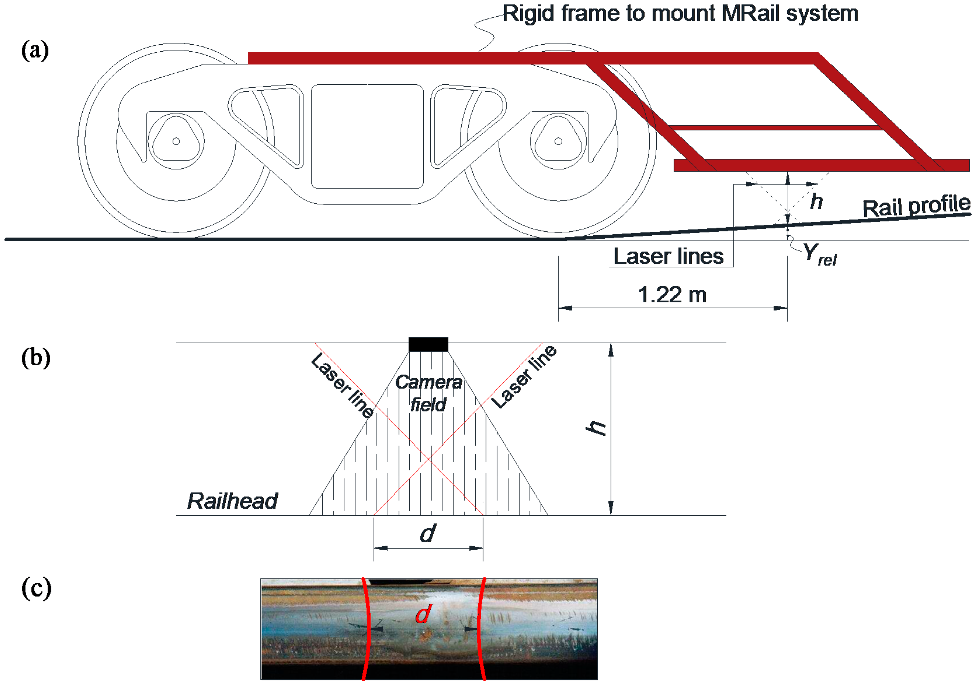
The MRail system was originally developed at the University of Nebraska–Lincoln under the sponsorship of the Federal Railroad Administration (FRA) [10,11,12]. The system measures the relative vertical deflection (Yrel) between the rail surface and the rail/wheel contact plane, at a distance of 1.22 m from the nearest wheel to the acquisition system (Figure 1a). The sensors consist of two laser lines and a digital camera mounted on the side frame of the rail car (Figure 1b). The laser system projects two curves on the rail surface, whose minimum distance (d) is captured by the camera (Figure 1c). Subsequently, the distance between the camera and the rail surface (h) is computed by converting d. Finally, the relative deflection Yrel is calculated by subtracting h from (Yrel + h), the fixed distance between the rail/wheel contact plane and the camera.
The MRail system can measure the deflection at different sampling rates with the speed up to 96 km/h (60 mph). The Winkler model and the finite element models have been used to estimate the track modulus from Yrel [24].
2.2. Winkler Model
Rail deformation and bending stress under specific loads are typically estimated using THE Winkler model, which considers the track as an infinite beam on a continuous elastic foundation [27,28,29]. Using the Winkler model (Equation (1)), the vertical rail deflection (y) at a distance x from the applied load (P) is computed as follows:
where β is the stiffness ratio, which is equal to (U/(4EI))0.25, U is the track modulus, E is the modulus of the elasticity of the rail, and I is the second moment of area of the rail.
From the Winkler model, the vertical deflection profile of a rail is only dependent on the track modulus value when the rail size and vertical loads are known. Once a value is assumed for track modulus, the rail vertical deflection profile can be estimated using Equation (1), and from the rail vertical deflection profile, Yrel can be calculated as the relative vertical deflection between the rail surface and the rail/wheel contact plane at a distance of 1.22 m from the nearest wheel (Figure 1a) [11,30]. The main shortcoming in this method is that the Winkler model assumes a track modulus is constant along the track while the field data shows that a track modulus stochastically varies along the track [31,32]. Therefore, the estimation of the track modulus from the Yrel measurements needs more advanced numerical models.
2.3. Finite Element Model
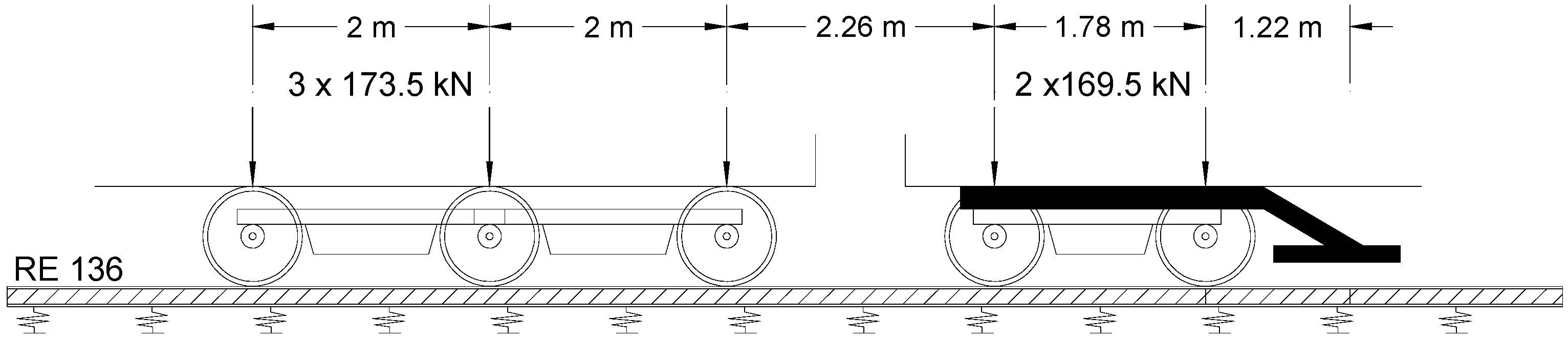
FEMs allow the simulation of a stochastically varying track modulus, and therefore, a more accurate simulation of Yrel measurements. Fallah Nafari et al., developed 90 FEMs with a stochastically varying track modulus to facilitate a more detailed investigation of the relationship between the Yrel and the track modulus [21]. Datasets from the 90 FEMs were used for the study in this paper. Hence, the details of the models are discussed briefly. The models are developed using CSiBridge software, where each model includes a 180.8 m track structure with two rails, crossties, and spring supports [33]. To develop each model, a normal track modulus distribution is assumed and randomly selected numbers from this distribution are assigned to the spring supports along the track. Statistical properties of the assumed normal distributions are summarized in Table 1, and the applied loads are depicted in Figure 2. RE136 rail size and 0.508 m tie spacings are used in the models.
Individual Yrel values are calculated from the vertical deflection profile at every 0.3048 m (1 ft) interval while the moving loads pass the track model. The dynamic effects of track–train interactions are not considered during the simulations due to the software’s limitation. This is acceptable within the scope of this study which mostly focuses on the Canadian freight lines where speeds are most likely lower than 65 km/h.
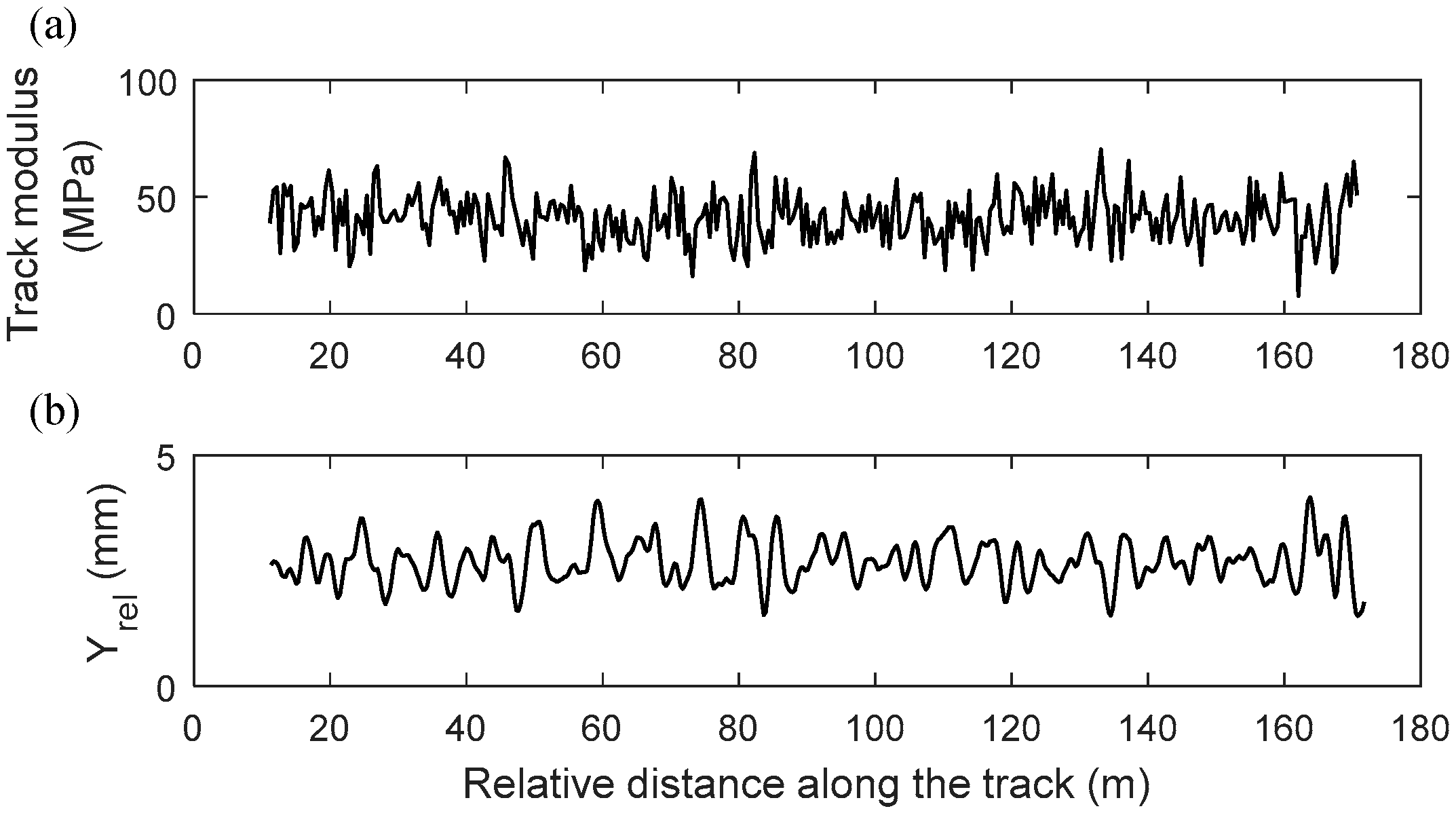
Figure 3 shows an example of the inputted track modulus to the model and corresponding Yrel output. Fallah Nafari et al., used basic statistical analysis and curve fitting approaches to study the relationship between the statistical properties of track modulus (U) and Yrel [21]. The results showed that the average and standard deviation of the track modulus over a track section length can be estimated from the average and standard deviation of Yrel over the same track section length. However, the estimation accuracy becomes lower by decreasing the track section length [21]. To overcome this shortcoming and increase the estimation accuracy of the track modulus, ANNs are proposed for the track modulus estimations in this study.
2.4. Estimation of Track Modulus Average
2.4.1. Multilayer Perceptron Artificial Neural Networks
Multilayer perceptron neural networks (MLPNN) are typically useful for classification, and function approximation problems [34,35,36,37,38]. The implementation of MLPNN is operated with two stages of performance, i.e., training and testing procedures. Once the training process is successfully performed in a self-adaptive manner with all defined parameters (such as learning algorithm and network architecture including several layers, and neurons in each layer), the network can effectively approximate the input–output mapping function.
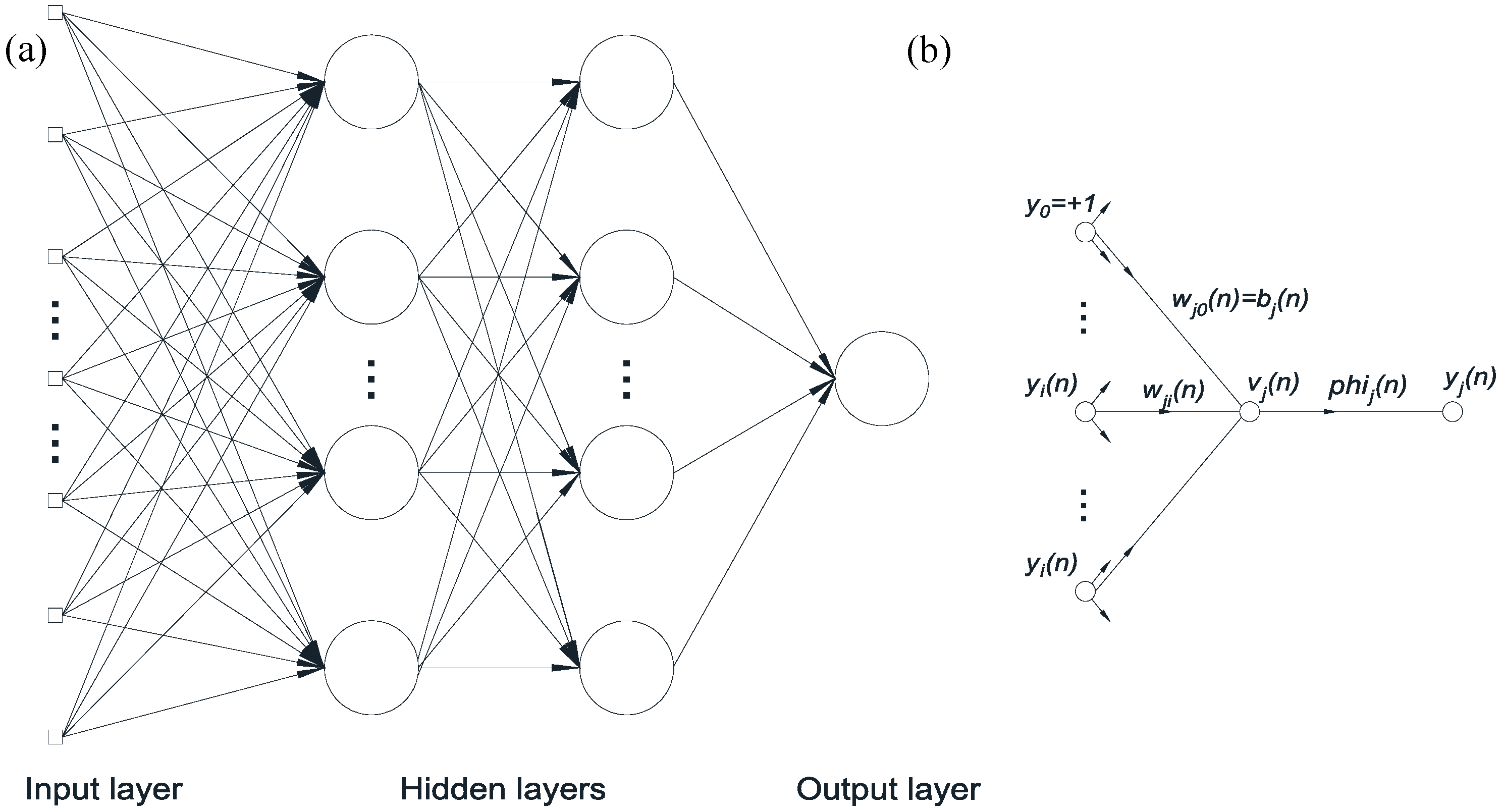
MLPNN is a network containing two or more neurons distributed in different layers, such as input layers, output layers, and hidden layers that connect the input and output layers (Figure 4a). Each neuron has a nonlinear differentiable activation function that creates real values and is highly connected to other neurons based on synaptic weights wij (n) (Figure 4b) as the level of connectivity.
One of the most complicated tasks before executing an MLPNN is that all the required parameters should be well defined to approximate the input–output relationship, which is called the learning process that contains two phases. In the forward phase, the inputs are fed into the network from left to right, and layer by layer with the fixed values of synaptic weights. In the backward phase, the error vector is first computed by subtracting the output of the network from the expected target. The error is then propagated backward from the output to the input layer. In this phase, the synaptic weights are adjusted to minimize the network error by solving the credit-assignment problems in the operation of each hidden unit. Each synaptic weight will be updated differently based upon the contribution of the corresponding hidden unit to the overall error. More information about training the network using backpropagation and gradient descent is in Haykin’s book [34].
2.4.2. Estimation Procedure and Results
The inputted track modulus and the corresponding Yrel data from the 180 m track models are divided into equivalent groups based on a track section length (e.g., 5 m, 10 m, etc.). Once the subgroups are defined, the average and standard deviation of Yrel in each subgroup are used as the networks’ inputs whereas the track modulus averages in the corresponding track segments are defined as the network’s outputs.
Yrel data extracted from eighty-one FEMs (out of ninety FEMs) are used to train the neural network. The accuracy of the trained network is then tested using the remaining nine (unseen) FEMs. These nine FEMs are called “unseen models” hereafter as they are not used in training the network. To test the trained network, track modulus average is estimated from Yrel average and the standard deviation for the nine unseen models. The estimated track modulus average is then compared with the track modulus inputted initially into the FEMs to generate Yrel data. The effectiveness of the proposed network is measured based on three parameters: the coefficient of determination (R2), the root mean square error (RMSE), and the mean absolute percentage error (MAPE) [39]. These measures are described as follows:
where ,,, and are the average and standard deviation of the estimated, and targeted values; N is the number of testing samples.
When a network is trained, five-fold cross-validation is employed to minimize any potential over-fitting problem and increase the network’s generalization. Regarding the network architecture, a network with two hidden layers (each contains 15 hidden nodes) is used in this study. This network ensures an acceptable error range, avoids over-fitting, and optimizes the computational efficiency. From different tests, it is noted that increasing the number of hidden nodes and hidden layers, does not necessarily mean the network’s performance is improved. In fact, the input configuration is the most important factor that controls the network performance.
Five networks for five different track section lengths have been fully trained to perform this study. The track modulus average over five section lengths is then estimated for the nine new models using the trained networks. Table 2 presents the accuracy level of these estimations. From the table, the network performs better when the track section length increases although the error is acceptably small even with the case of a 10 m section length. R2 is 0.95 for the case of the 10 m section length, which means that the estimated and inputted track modulus averages are well correlated. Moreover, the RMSE and MAPE are quite small, i.e., 2.81 MPa, and 6.99% respectively, considering that range of inputted track modulus average is 12.8 to 41.4 MPa. In addition to confirming the applicability of the Yrel data in indicating the track modulus information, the current methodology provides more accurate results than the other method in the literature [21]. As shown in Table 2, the R2 value computed in the related study decreases as the length of the track segment reduces, whereas the R2 in the current study is almost constant for cases with a 10 m track section and more.
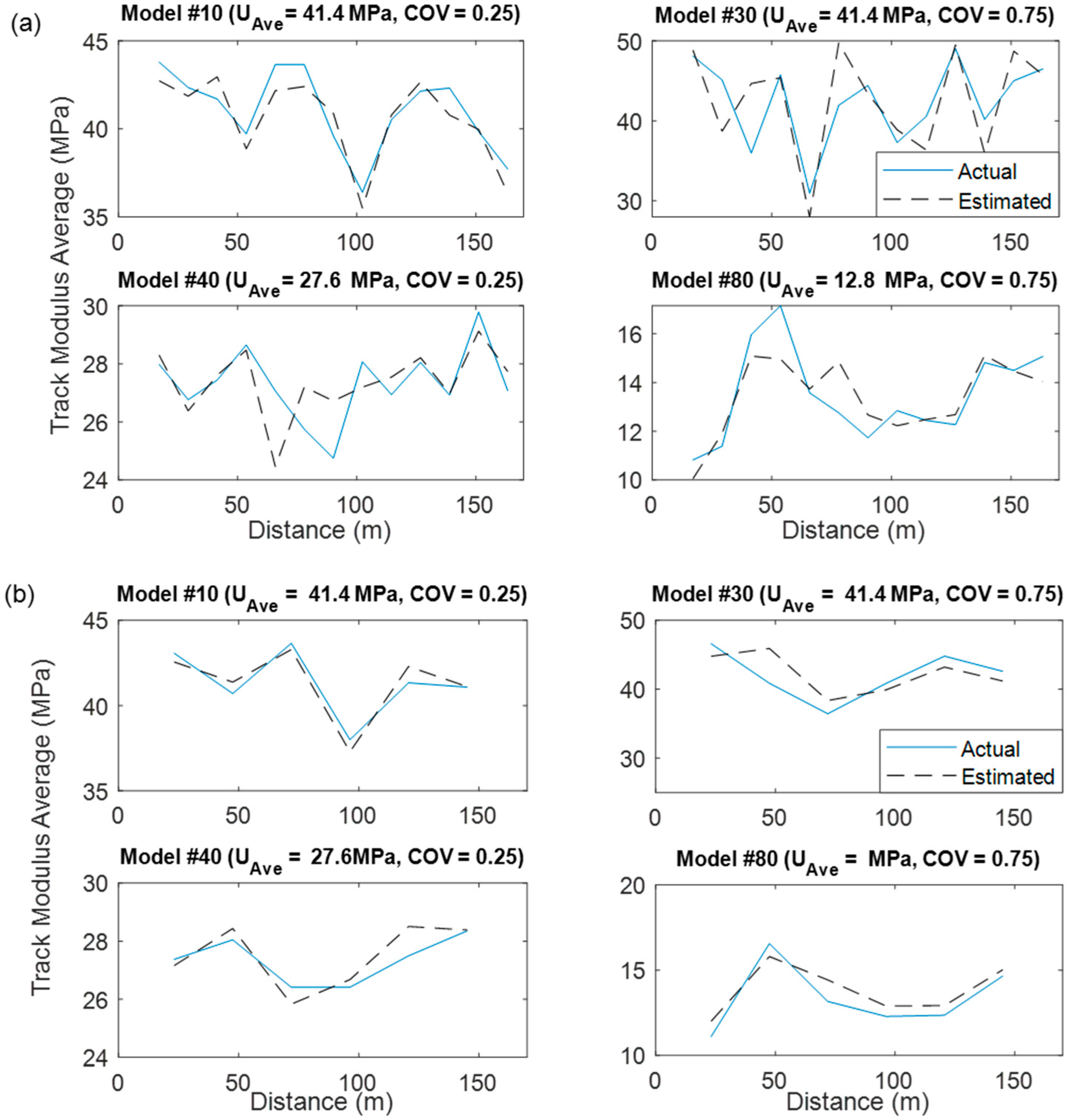
The accuracy of the estimation method for the case of the 10 and 20 m section lengths are demonstrated in Figure 5 for four models as an example. These four models had a different track modulus average and variations. From the figure, the values estimated from the networks are very close to the actual track modulus average inputted to the FEMs. Better results can be observed in the case of a 20 m section length (Figure 5b) although the performance of the estimation of track modulus over the shorter section length (Figure 5a) is still satisfactory. Most importantly, the local fluctuation of the track modulus is well captured.
The effectiveness of the framework is further investigated by adding artificial noise to the Yrel data extracted from the FEMs. This simulates the real-life condition in which the Yrel measurements are affected by parameters such as the resolution of the MRail measurement system, track irregularities, etc. The artificial noise was added based on Equation (5) [40]. An example of pure vs. noise-added Yrel is shown in Figure 6:
where α, and β are random numbers ranging from −1 to 1.
The noisy Yrel is used to train new networks, and then the trained networks are used to estimate the track modulus average. The estimated track modulus is then compared with the inputted track modulus for each model and the error is reported in Table 3. From the table, the estimation of the track modulus average (Uave) from the noisy Yrel is still successful even for the short track section length of 10 m as R2 is 0.95, and RMSE is 2.77 MPa. This demonstrates that the framework performs effectively even when the Yrel data contain noise, and thus is expected to work with real-life data.
2.5. Estimation of Track Modulus Standard Deviation (USD)
The estimation of the track modulus standard deviation from the Yrel data using statistical methods and curve-fitting approaches has not been successful for track section lengths shorter than 80 m [21]. Therefore, frequency characteristics of the deflection data are investigated in this study to increase the estimation accuracy of track modulus standard deviation. The coefficients associated with the Yrel frequency components are employed as one of the inputs to the ANNs, whose outputs are the track modulus standard deviation over different track section lengths. As demonstrated in Figure 7, Yrel and the track modulus data are divided into different subgroups based on various track section lengths (similar to the procedure used for estimating the track modulus average). Then, statistical analysis, fast Fourier transform, and a liftering technique are applied on the Yrel data in each subgroup to extract the average and standard deviation of the Yrel and average and the standard deviation of liftering the fast Fourier transform (FFT) coefficients. These parameters are used as the inputs of ANNs.
Figure 8a shows an example of the FFT coefficients of the Yrel data over a track section of 30 m for 81 models. As can be seen, the coefficients at higher orders are relatively small. This is undesirable for training the ANN due to possible bias. Therefore, the coefficients are processed using a liftering technique (Equation (6) to roughly normalize their variances) [41]:
where L is the sin lifter parameter, which is 50 in the current study, and X(k) is the FFT coefficients.
Once the liftering technique is applied (Figure 8b), the average and standard deviations of the lifted FFT are calculated using Equations (7) and (8) are used as two additional inputs for ANNs.
The architecture used for developing the network in this section has two hidden layers and 15 hidden nodes in each layer, similar to the network’s architecture for estimating the track modulus average. The trained networks are used for estimating the track modulus standard deviation over different track section lengths and three accuracy measurements are reported in Table 4. In order to show that the current input–output pair is optimized, and two network architectures are trained (ANN-1 with four inputs, i.e., the average and standard deviation of Yrel, and the average and standard deviation of the lifted FFT; ANN-2 with two inputs, i.e., mean and standard deviation of Yrel). In each case, the two networks are trained and tested multiple times and the mean and standard deviation of the performance parameters are computed and reported in Table 4. For the case of 5 m section length, for instance, the networks’ input, and output are first extracted based on the chosen section (5 m), then ANN-1 and ANN-2 networks are trained using the training data and tested against the data extracted from nine unseen FEMs.
From Table 4, the error values show that the standard deviation of track modulus (USD) can be estimated satisfactorily by both network configurations (ANN-1 and ANN-2). Even for the 10-m section length case, for instance, the coefficient of correlations between the actual USD and the one estimated by the two networks are very high, e.g., 0.83 and 0.82 respectively. However, the networks with four inputs (ANN-1) slightly outperform the one with two inputs (ANN-2) regardless of the section lengths. Specifically, the RMSE and MAPE are always smaller than those arising from the trained networks whose inputs are the statistical properties of Yrel only (ANN-2). Values estimated using the networks with four inputs have relatively high R2 in all cases showing that the methodology is successful. In particular, the R2 is as high as 0.94 for the case of the 25 m section length and the RMSE is 1.83 MPa, which is a relatively small error considering that the maximum standard deviation of the inputted track modulus in the FEMs is 31.05 MPa. Moreover, the first network (ANN-1) provides more reliable results as the standard deviation of RMSE remains stable (varying from 0.11 to 0.17 MPa) and lower than those of ANN-2. Therefore, combining FFT and statistical analysis to configure the input for the networks noticeably improves the estimation accuracy, and increases the stability of the ANNs, the mapping function between the Yrel characteristics and the track modulus standard deviation (USD). Most importantly, there is a big step forward in this paper compared to the previous study, where the R2 coefficient is 0.748 even though the 40 m section length is used [21]. The performance of this estimation can be considered ineffective as the R2 coefficient reduced significantly in shorter track segment cases (Table 4). Hence, considering the current results, it can be claimed that neural networks are more powerful for mapping the relationship between Yrel and track modulus, especially over the short track section lengths.
For more descriptive results, the strong correlation between the actual and estimated track modulus’s standard deviation for the 25 m section length is demonstrated in Figure 9. As can be seen, the estimated standard deviations follow the same patterns as those of the actual values, which vary greatly from 3.2 to 31.05 MPa.
The effectiveness of the methodology is further validated by adding noise into the deflection data (Yrel). Similar to the procedure mentioned in the previous section, noise is added to the Yrel data from 90 models using Equation ((5). The dataset from 81 models is then used to train the networks using two approaches: networks with two inputs (average and standard deviation of Yrel) and networks with four inputs (average and standard deviation of Yrel and average and standard deviation of the lifted FFT). The developed networks are used to estimate the track modulus standard deviations over the different section lengths from the unseen Yrel data. The estimated values are compared with the standard deviation of track modulus inputted to FEMs and results are reported in Table 5. The results show that the proposed approaches work very well even when Yrel datasets are affected by noises. The R2 is again higher than 0.90 when the 25 m or higher section lengths are utilized.
3. Conclusions
In this paper, two frameworks are proposed for estimating the track modulus average, and the standard deviation over the different track section lengths. The frameworks employed Yrel data (a relative rail vertical deflection measured using the MRail system) for the track modulus estimations. The relationship between the statistical properties of the track modulus and the Yrel data were investigated using artificial neural networks (ANNs). Datasets from FEMs are used to train the ANNs in which their outputs are either the track modulus average or standard deviations. Both statistical and frequency analyses were conducted to identify the optimized inputs for the ANNs from the Yrel data. From the results, the track modulus average over a track section length of 10 m or longer is accurately estimated from the average and standard deviation of the Yrel data within the corresponding section length. Additionally, the standard deviation of the track modulus over a section length of 25 m or longer is estimated with an acceptable level of accuracy. It is also shown that the trained ANNs work very well for the track modulus estimations even when the Yrel values as the ANN inputs are affected by noise. The proposed ANNs are only applicable to a specific rail type and loading condition. Hence, a similar procedure should be followed to train the ANNs for different ranges of rail sections and loading types.
Author Contributions
Conceptualization, N.T.D., M.G. and S.F.N.; methodology, N.T.D.; software, N.T.D., S.F.N.; validation, N.T.D., M.G. and S.F.N.; formal analysis, N.T.D., M.G.; writing—original draft preparation, N.T.D.; writing—review and editing, N.T.D., M.G. and S.F.N.; supervision, M.G. All authors have read and agreed to the published version of the manuscript.
Funding
The study is funded by IC-IMPACTS (the India-Canada Centre for Innovative Multidisciplinary Partnerships to Accelerate Community Transformation and Sustainability), established through the Networks of Centres of Excellence of Canada.
Conflicts of Interest
The authors declare no conflict of interest.
References
- Selig, E.T.; Li, D. Track modulus: Its meaning and factors influencing it. Transp. Res. Rec. 1994, 1470, 47–54. [Google Scholar]
- Ebersohn, W.; Selig, E.T. Track modulus measurements on a heavy haul line. Transp. Res. Rec. 1994, 1470, 73. [Google Scholar]
- Lopez Pita, A.; Teixeira, P.F.; Robuste, F. High Speed and Track Deterioration: The Role of Vertical Stiffness of the Track. Proc. Inst. Mech. Eng. Pt. F J. Rail Rapid Transit. 2004, 218, 31–40. [Google Scholar] [CrossRef]
- Dahlberg, T. Railway Track Stiffness Variations-Consequences and Countermeasures. Int. J. Civ. Eng. 2010, 8, 1–12. [Google Scholar]
- Sussmann, T.R.; Ebersohn, W.; Selig, E.T. Fundamental nonlinear track load-deflection behavior for condition evaluation. Transp. Res. Rec. 2001, 61–67. [Google Scholar] [CrossRef]
- Burrow, M.P.N.; Chan, A.H.C.; Shein, A. Deflectometer-based analysis of ballasted railway tracks. Proc. Inst. Civ. Eng. Geotech. Eng. 2007, 160, 169–177. [Google Scholar] [CrossRef]
- Norman, C.; Farritor, S.; Arnold, R.; Elias, S.; Fateh, M.; El-Sibaie, M. Design of a System to Measure Track Modulus from a Moving Railcar; US Department of Transportation, Federal Railroad Administration, Office of Research and Development: Washington, DC, USA, 2006; paper ID 20590.
- Eric, G.B.; Nissen, A.; Björn, S.P. Track deflection and stiffness measurements from a track recording car. Proc. Inst. Mech. Eng. Pt. F J. Rail Rapid Transit. 2014, 228, 570–580. [Google Scholar] [CrossRef]
- Wang, P.; Wang, L.; Chen, R.; Xu, J.; Xu, J.; Gao, M. Overview and outlook on railway track stiffness measurement. J. Mod. Transp. 2016, 24, 89–102. [Google Scholar] [CrossRef] [Green Version]
- Lu, S. Real-Time Vertical Track Deflection Measurement System. Ph.D. Thesis, University of Nebraska Lincoln (UNL), Lincoln, Nebraska, 2008. [Google Scholar]
- Norman, C.D. Measurement of Track Modulus from a Moving Railcar. Master’s Thesis, University of Nebraska-Lincoln, Lincoln city, NE, USA, 2004. [Google Scholar]
- Greisen, C.J. Measurement, Simulation, and Analysis of the Mechanical Response of Railroad Track. Master’s Thesis, University of Nebraska-Lincoln, Lincoln city, NE, USA, 2010. [Google Scholar]
- Thompson, R.; Li, D. Automated vertical track strength testing using TTCI’s track loading vehicle. Technol. Digest. 2002, 1489, 17–25. [Google Scholar]
- Li, D.; Thompson, R.; Marquez, P.; Kalay, S. Development and Implementation of a Continuous Vertical Track-Support Testing Technique. Transp. Res. Rec. 2004, 1863, 68–73. [Google Scholar] [CrossRef]
- Rasmussen, S.; Krarup, J.A.; Hildebrand, G. Non-Contact Deflection Measurement at High Speed. In Proceedings of the 6th International Conference on the Bearing Capacity of Roads, Railways and Airfields, Lisbon, Portugal, 24–26 June 2002. [Google Scholar]
- Berggren, E.G.; Kaynia, A.M.; Dehlbom, B. Identification of substructure properties of railway tracks by dynamic stiffness measurements and simulations. J. Sound Vib. 2010, 329, 3999–4016. [Google Scholar] [CrossRef]
- With, C.; Metrikine, A.V.; Bodare, A. Identification of effective properties of the railway substructure in the low-frequency range using a heavy oscillating unit on the track. Arch. Appl. Mech. 2010, 80, 959–968. [Google Scholar] [CrossRef] [Green Version]
- Roghani, A.; Hendry, M.; Ruel, M.; Edwards, T.; Sharpe, P.; Hyslip, J. A case study of the assessment of an existing rail line for increased traffic and axle loads. In Proceedings of the IHHA 2015 Conference, Peth, Australia, 21–24 June 2015. [Google Scholar]
- Roghani, A.; Hendry, M.T. Assessing the potential of a technology to map the subgrade stiffness under the rail tracks. In Proceedings of the Transportation research board 94th annual meeting; Transportation Research Board, Washington, DC, USA, 11–15 January 2015. [Google Scholar]
- Roghani, A.; Macciotta, R.; Hendry, M. Combining track quality and performance measures to assess track maintenance requirements. In Proceedings of the ASME/ASCE/IEEE 2015 Joint Rail Conference, American Society of Mechanical Engineers, San Jose, CA, USA, 23–26 March 2015. [Google Scholar]
- Fallah Nafari, S.; Gül, M.; Roghani, A.; Hendry, M.T.; Cheng, J.R. Evaluating the potential of a rolling deflection measurement system to estimate track modulus. Proc. Inst. Mech. Eng. Pt. F J Rail Rapid Transit. 2018, 232, 14–24. [Google Scholar] [CrossRef]
- Mehrali, M.; Esmaeili, M.; Mohammadzadeh, S. Application of data mining techniques for the investigation of track geometry and stiffness variation. Proc. Inst. Mech. Eng. Pt. F J Rail Rapid Transit. 2019, 234, 439–453. [Google Scholar] [CrossRef]
- Lu, S.; Hogan, C.; Minert, B.; Arnold, R.; Farritor, S.; GeMeiner, W.; Clark, D. Exception criteria in vertical track deflection and modulus. In 2007 ASME/IEEE Joint Rail Conference and the ASME Internal Combustion Engine Division, Spring Technical Conference (JRCICE 2007); American Society of Mechanical Engineers: Pueblo, CO, USA, 2007; pp. 191–198. [Google Scholar]
- El-Sibaie, M.; GeMeiner, W.; Clark, D.; Al-Nazer, L.; Arnold, R.; Farritor, S.; Fateh, M.; Lu, S.; Carr, G. Measurement of Vertical Track Modulus: Field Testing, Repeatability, and Effects of Track Geometry. In Proceedings of the ASME/IEEE Joint Rail Conference, Wilmington, DE, USA, 22–24 April 2009; pp. 151–158. [Google Scholar]
- Alireza, R.; Hendry, M.T. Continuous Vertical Track Deflection Measurements to Map Subgrade Condition along a Railway Line: Methodology and Case Studies. J. Transp. Eng. 2016, 142, 04016059. [Google Scholar] [CrossRef]
- Fallah Nafari, S.; Gül, M.; Hendry, M.T.; Cheng, J.R. Estimation of vertical bending stress in rails using train-mounted vertical track deflection measurement systems. Proc. Inst. Mech. Eng. Pt. F J Rail Rapid Transit. 2018, 232, 1528–1538. [Google Scholar] [CrossRef]
- Sadeghi, J.; Barati, P. Evaluation of conventional methods in Analysis and Design of Railway Track System. IJCE 2010, 8, 44–56. [Google Scholar]
- Esveld, C. Modern Railway Track; MRT Productions: Duisburg, Germany, 1989; p. 446. [Google Scholar]
- Feng, H. 3D-Models of Railway Track for Dynamic Analysis; Royal Institute of Technology: Stockholm, Sweden, 2011. [Google Scholar]
- Fallah Nafari, S.; Gül, M.; Cheng, J.J.R. Quantifying live bending moments in rail using train-mounted vertical track deflection measurements and track modulus estimations. J. Civ. Struct. Health Monit. 2017, 7, 637–643. [Google Scholar] [CrossRef]
- Zakeri, J.A.; Abbasi, R. Field investigation on variation of rail support modulus in ballasted railway tracks. Lat. Am. J. Solids Struct. 2012, 9, 643–656. [Google Scholar] [CrossRef] [Green Version]
- Sussmann, T.R.; Thompson, H.B.; Stark, T.D.; Wilk, S.T.; Ho, C.L. Use of seismic surface wave testing to assess track substructure condition. Constr. Build. Mater. 2017, 155, 1250–1255. [Google Scholar] [CrossRef]
- Bridge, C. Computers and Structures; CSI: Berkeley, CA, USA, 2015. [Google Scholar]
- Haykin, S.S. Neural Networks and Learning Machines; Prentice Hall: New York, NY, USA, 2009; p. 906. [Google Scholar]
- Cybenko, G. Approximation by superpositions of a sigmoidal function. Math. Control Signals Syst. 1989, 2, 303–314. [Google Scholar] [CrossRef]
- Guler, H. Prediction of railway track geometry deterioration using artificial neural networks: A case study for Turkish state railways. Struct. Infrastruct. Eng. 2014, 10, 614–626. [Google Scholar] [CrossRef]
- Fink, O.; Weidmann, U. Scope and potential of applying artificial neural networks in reliability prediction with a focus on railway rolling stock. In European Safety and Reliability Conference: Advances in Safety, Reliability and Risk Management, ESREL 2011; Taylor and Francis Inc.: Troyes, France, 2012; pp. 508–514. [Google Scholar]
- Sadeghi, J.; Askarinejad, H. Application of neural networks in evaluation of railway track quality condition. J. Mech. Sci. Technol. 2012, 26, 113–122. [Google Scholar] [CrossRef]
- Hyndman, R.J.; Koehler, A.B. Another look at measures of forecast accuracy. Int. J. Forecast 2006, 22, 679–688. [Google Scholar] [CrossRef] [Green Version]
- Fallah Nafari, S. Quantifying the Distribution of Rail Bending Stresses along the Track Using Train-Mounted Deflection Measurements; University of Alberta: Edmonton, AB, Canada, 2017. [Google Scholar]
- Young, S.; Evermann, G.; Gales, M.; Hain, T.; Kershaw, D.; Liu, X.; Moore, G.; Odell, J.; Ollason, D.; Povey, D. The HTK Book; Cambridge University Engineering Department: Cambridge, UK, 2006. [Google Scholar]
Figure 1.
Demonstration of the MRail system (real-time vertical track deflection measurement system) for Yrel measurements: (a) the measurement system on a rigid frame; (b) the sensor system; and (c) the projections of the laser lines on the railhead.
Figure 1.
Demonstration of the MRail system (real-time vertical track deflection measurement system) for Yrel measurements: (a) the measurement system on a rigid frame; (b) the sensor system; and (c) the projections of the laser lines on the railhead.

Figure 2.
The loading condition in the finite element models (FEMs).

Figure 3.
(a) Track modulus inputted to the FEM (Mean = 41.4 MPa, COV = 0.25); and (b) the extracted Yrel.
Figure 3.
(a) Track modulus inputted to the FEM (Mean = 41.4 MPa, COV = 0.25); and (b) the extracted Yrel.

Figure 4.
(a) Example of a two-hidden layer perceptron; (b) typical operation at neuron j.

Figure 5.
Moving average of the actual track modulus inputted to the FEMs vs. estimated values over: (a) the 10 m section length; and (b) the 20 m section length.
Figure 5.
Moving average of the actual track modulus inputted to the FEMs vs. estimated values over: (a) the 10 m section length; and (b) the 20 m section length.

Figure 6.
Demonstration of pure and noisy Yrel.

Figure 7.
Procedure for estimating the track modulus standard deviation (USD).

Figure 8.
FFT of Yrel: (a) before liftering; and (b) after liftering.

Figure 9.
The actual track modulus standard deviation over the 25 m section length vs. the estimated values.
Figure 9.
The actual track modulus standard deviation over the 25 m section length vs. the estimated values.


Table 1.
Statistical properties of the track modulus in the FEMs.
| Track Modulus Average (MPa) | Coefficient of Variation (COV) | No. of Simulations |
|---|---|---|
| 41.4 | 0.25; 0.5; 0.75 | 30 (10 simulations for each COV) |
| 27.6 | 0.25; 0.5; 0.75 | 30 (10 simulations for each COV) |
| 12.8 | 0.25; 0.5; 0.75 | 30 (10 simulations for each COV) |
Table 2.
Estimation accuracy of the track modulus average (no noise added).
| Section Length (m) | MAPE * (%) | RMSE ** (MPa) | R2 | R2 in [21] |
|---|---|---|---|---|
| 5 | 12.42 | 4.58 | 0.86 | 0.79 |
| 10 | 6.99 | 2.81 | 0.95 | 0.93 |
| 15 | 5.90 | 2.56 | 0.95 | N/A |
| 20 | 4.32 | 1.60 | 0.98 | 0.96 |
| 25 | 3.87 | 1.63 | 0.98 | N/A |
* Mean Absolute Percentage Error; ** Root Mean Square Error.
Table 3.
Estimation accuracy of the track modulus average (with added noise).
| Section Length (m) | MAPE (%) | R2 | RMSE (MPa) | R2 in [21] |
|---|---|---|---|---|
| 5 | 14.09 | 0.83 | 5.07 | 0.79 |
| 10 | 7.01 | 0.95 | 2.77 | 0.93 |
| 15 | 5.93 | 0.96 | 2.36 | - * |
| 20 | 6.07 | 0.97 | 1.98 | 0.96 |
| 25 | 3.98 | 0.98 | 1.53 | - * |
* Not available for comparisons since those section lengths are not available in the previous study.
Table 4.
Estimation accuracy of the USD (no noise added, the standard deviation in the parenthesis).
Table 4.
Estimation accuracy of the USD (no noise added, the standard deviation in the parenthesis).
| Section Length (m) | Network Configuration | RMSE (MPa) | MAPE (%) | R2 | R2 in [21] |
|---|---|---|---|---|---|
| 10 | ANN-1 | 3.00 (0.16 *) | 18.41 | 0.83 | 0.53 |
| ANN-2 | 3.05 (0.22) | 19.12 | 0.82 | - | |
| 15 | ANN-1 | 2.36 (0.08) | 15.01 | 0.89 | - |
| ANN-2 | 2.61 (0.39) | 15.79 | 0.87 | - | |
| 20 | ANN-1 | 2.23 (0.11) | 14.49 | 0.91 | 0.66 |
| ANN-2 | 2.59 (0.89) | 14.47 | 0.88 | - | |
| 25 | ANN-1 | 1.83 (0.13) | 11.96 | 0.94 | - |
| ANN-2 | 1.99 (0.30) | 11.72 | 0.92 | - | |
| 30 | ANN-1 | 2.08 (0.17) | 11.61 | 0.92 | - |
| ANN-2 | 2.14 (0.44) | 11.79 | 0.91 | - |
* Standard deviation of the estimation error.
Table 5.
Estimation accuracy of the USD (with noise added).
| Section Length (m) | Network Configuration | R2 | RMSE (MPa) | MAPE (%) |
|---|---|---|---|---|
| 10 | ANN-1 | 0.82 | 3.06 | 20.12 |
| ANN-2 | 0.81 | 3.14 | 19.64 | |
| 15 | ANN-1 | 0.87 | 2.59 | 16.30 |
| ANN-2 | 0.87 | 2.64 | 16.23 | |
| 20 | ANN-1 | 0.89 | 2.42 | 16.13 |
| ANN-2 | 0.89 | 2.45 | 14.71 | |
| 25 | ANN-1 | 0.94 | 1.86 | 11.96 |
| ANN-2 | 0.93 | 1.88 | 11.73 | |
| 30 | ANN-1 | 0.94 | 1.84 | 10.43 |
| ANN-2 | 0.93 | 1.89 | 10.95 |
© 2020 by the authors. Licensee MDPI, Basel, Switzerland. This article is an open access article distributed under the terms and conditions of the Creative Commons Attribution (CC BY) license (http://creativecommons.org/licenses/by/4.0/).
Share and Cite
MDPI and ACS Style
Do, N.T.; Gül, M.; Nafari, S.F. Continuous Evaluation of Track Modulus from a Moving Railcar Using ANN-Based Techniques. Vibration 2020, 3, 149-161. https://0-doi-org.brum.beds.ac.uk/10.3390/vibration3020012
AMA Style
Do NT, Gül M, Nafari SF. Continuous Evaluation of Track Modulus from a Moving Railcar Using ANN-Based Techniques. Vibration. 2020; 3(2):149-161. https://0-doi-org.brum.beds.ac.uk/10.3390/vibration3020012
Chicago/Turabian StyleDo, Ngoan T., Mustafa Gül, and Saeideh Fallah Nafari. 2020. "Continuous Evaluation of Track Modulus from a Moving Railcar Using ANN-Based Techniques" Vibration 3, no. 2: 149-161. https://0-doi-org.brum.beds.ac.uk/10.3390/vibration3020012