Benchmarking Wind Farm Projects by Means of Series Two-Stage DEA


School of Applied Mathematics and Physics, National Technical University of Athens, 15780 Athens, Greece
Clean Technol. 2020, 2(3), 365-376; https://0-doi-org.brum.beds.ac.uk/10.3390/cleantechnol2030022
Submission received: 31 May 2020
/
Revised: 20 August 2020
/
Accepted: 27 August 2020
/
Published: 4 September 2020
(This article belongs to the Special Issue Feature Papers 2020)
Abstract
:This paper presents a data envelopment analysis (DEA) approach to benchmark a group of wind farm (WF) projects in Greece by employing a series two-stage structure. In the first stage, the investment performance of projects is evaluated using contract data and site wind conditions, though in the second stage the WF operational efficiency is evaluated using data on production inputs and output. Inefficiency occurs in both the construction and operating stages, but the construction process appears to be more inefficient relative to the operating phase. Moreover, WF size is related to operating efficiency and sensitivity analysis results identify wind speed and WF installation capacity as the factors that affect the investment performance and operational efficiency, respectively. The proposed approach is an addition to the existing literature and it can be used by managers and facility operators.
1. Introduction
Renewable energy production has been increased rapidly over the last few years and wind energy production has made an important contribution to this development [1]. Wind energy is produced by onshore or offshore wind farms (WFs) that are groups of wind turbines (WTs) located in the same place. Wind energy is deemed a mature and cost-competitive source of electricity production in Europe that contributes to the security and sustainability of the energy system [2]. Europe installed 15.4 GW (13.2 GW in the EU) of new wind power capacity (mainly onshore WFs) in 2019 and reached 205 GW of wind energy cumulative capacity; wind energy accounted for 15% of the electricity consumption in the EU-28 in 2019. In Greece the new onshore installations in 2019 were about 0.7 GW, whereas the cumulative onshore installed capacity reached about 3.6 GW; the percentage of the electricity demand covered by wind energy in 2019 was 12%. According to data on fourteen countries the average power rating of onshore turbines in Europe is 3.1 MW, whereas in Greece the average power rating is 2.3 MW [3].
A WT’s efficiency evaluation can be carried out using [4]: (i) the annual energy output (AEP), (ii) the power curve, and (iii) the power coefficient. To measure a WT’s productive efficiency as the ratio of current performance to best performance, a benchmark is required that represents the best performance attainable. The use of AEP is inappropriate because wind conditions influence power production, and it is difficult to adjust these conditions to comparable levels in real applications. In addition, power curve and power coefficient are both average output metrics, and are thus not deemed suitable. The shortcomings of the above metrics have driven researchers to look for benchmarks in the field of production economics [4]. The measurement of efficiency is focused on estimating a production function using input and output data for a set of production units which may be WTs or WFs in the context of wind energy.
The productive efficiency of wind energy facilities is dependent on wind conditions, i.e., wind speed and wind power density at the production site, and other factors such as implantation and generation costs, and turbine productivity. Except for the above factors, profitability is determined by also taking into account the energy prices. Investments in WFs may attain high returns on investments because, in many countries, producers can take advantage of the above market guaranteed wind energy price. It is evident that production inefficiency can reduce the profitability of WFs, thus the measurement of productive efficiency is essential [1].
Competitive approaches are used to assess the performance of WF projects such as the parametric stochastic frontier analysis (SFA) [5,6] and the non-parametric data envelopment analysis (DEA) [7]. SFA includes the selection of a functional type for production or cost frontier function, estimated econometrically, using two error term components, namely statistical noise and inefficiency. The normal and half-normal assumptions for noise and inefficiency are usually made for these terms, respectively.
In frontier efficiency analysis, given a group of j (= 1, …, n) observations on homogeneous entities that generate one output y using a vector of m inputs xj = (x1, …, xm) Equations (1) and (2), respectively are assumed to provide frontier and observed production function [8]:
where, is the deterministic component and is an error term.
Different distributional assumptions set on that represent deviations from the frontier lead to different models [8]: (i) If such that yf ≥ y for all observations, then the frontier is deterministic and DEA can be used. (ii) If is a two-error term of noise and inefficiency then the frontier is stochastic and SFA should be used.
DEA, published by Charnes et al. [9] in the literature, is a mathematical programming technique that is used to determine the efficiency of a group of decision-making units (DMUs), in this case WFs. Efficiency ratings based on DEA take values between zero and unity (i.e., perfect efficiency for units located on the border); units located off the frontier are considered inefficient. With regard to WFs, it is necessary to identify two phases related to performance evaluation: the phase of construction (i.e., investment) prior to start-up, and the phase of operation. These stages are related to the evaluation ex ante and ex post [7], respectively.
The current study focuses on DEA which is more flexible than SFA and can be used to assess power facilities’ construction and operating phase [10]. There is a lack of studies assessing the WF projects’ DEA-based efficiency with a focus on the investment and operational stage. In this context, the current research aims at improving a single black box DEA [11] and evaluating the performance of a group of WF projects in Greece using a series two-stage DEA.
This research adds to the existing literature in several ways. Firstly, it provides new empirical evidence on the performance of investment and operational stages of WF projects. Second, it fills the gap produced by the single DEA black-box model for WF projects, using a DEA series two-stage model structure to assess both investment and operational efficiency. It determines for a group of Greek WFs to what extent the performance of projects could be improved in the construction phase by reducing selected inputs given the output and whether the WF operators could increase the produced electricity given the inputs. Moreover, WF performance and size are studied, and sensitivity analysis is conducted to provide more insight into the factors influencing WF performance.
Projects are seen as systems whose monitoring is based on the principles of the triangle of project management (i.e., schedule, cost, and quality). Using DEA, project efficiency is measured employing a results-oriented methodology based on the above principles [10]. In the case of the DEA-based assessment of power plants, performance in the investment and operating process can be separately differentiated and modeled [12].
The WF project assessment studies by DEA are divided into single-, two-stage and serial two-stage works. WFs are specified as DMUs in the works reviewed below. The classic single-stage DEA studies evaluate WFs within a black-box context in which the power facility is treated as a whole (i.e., black box) system without throwing light onto its structure [11]. Sarıca and Or [12] propose DEA models for the operational and investment performance of a group of Turkey’s thermal, hydro and wind power stations. In Greece, Champilomatis [13] assesses the performance of a group of 13 WFs. Kim et al. [14] evaluate the efficiency of the investment for renewable energy in Korea and Akbari et al. [15] perform a cross-European DEA-based efficiency assessment of offshore wind farms. Rodríguez et al. [16] provide an empirical DEA-based study of the evolution of total factor productivity among Spanish wind farms by deriving the Malmquist productivity index.
The two-stage studies measure the efficiency through DEA in the first stage, and then regress it in the second stage on explanatory variables [17]. Two-stage studies typically incorporate DEA and Tobit regression, such as Iglesias et al. [7] research on WF performance assessment in Spain, and Wu et al. [18] and Sağlam’s [19] works on WF performance assessment in China and Texas. Ederer [20] evaluates the performance of offshore WFs by also employing the two-stage DEA.
In another research strand, model building is based on the series two-stage DEA. Unlike the single DEA black-box model, a two-series DEA series structure distinguishes sub-processes and aims to calculate their efficiency [11]. In this strand lies the work of Niu et al. [21] proposing a DEA approach with a two series structure to evaluate the performance of WTs. It is worth noting that a series two-stage DEA can also be combined with Tobit regression [21]. With regard to explanatory variables, in a different modeling approach [22], they can be considered as inputs but are not active in the optimization process for the definition of the efficiency metrics. Examples of these explanatory variables which are deemed exogenous are the solar irradiance and ambient air temperature for the case of photovoltaic systems [23]. In a different setting, Sağlam [24] evaluates the US states’ wind power performances for electricity generation by employing the two-stage DEA approach and treating individual states as DMUs. DEA can also be combined with other methods such as SFA [7], life cycle assessment (LCA) [25] and emergy analysis [2].
Single- and two-stage DEA have been already employed for ex-post evaluation of WF projects. To the best of the author’s knowledge, a DEA-based assessment of the performance of WF projects in Greece by employing a series two-stage structure has not been implemented so far. The current study aims to fill this gap by adopting this structure to evaluate the efficiency of a group of WF projects ex-post and to open the black box by identifying the investment and operational stages in a DEA setting. Moreover, the current research is the first attempt to evaluate the performance of a group of WFs in Greece by distinguishing discretionary (i.e., controllable) and non-discretionary inputs.
2. Problem Statement
A number of WF projects may be over budget in the construction phase or unproductive during operation. An assessment of the performance of a WF project group is based on data analysis and benchmarks. The benchmarks (i.e., best-in-class WF projects) for the investment and operational stages can be established by means of DEA and moreover, their use as points of reference is essential for planning necessary interventions to improve performance. Corrective actions to improve performance should focus not only on the budgeting process in the investment stage but also on the optimization of production in the operating stage with the aim of maximizing the produced electricity. Thus, for WF projects, benchmarks should be established for the investment and operating stage.
It should be noted that the assumption of the existence of a local transmission grid should be made in the case of power facilities [10]. Since the WFs evaluated in the current study are in operation, they are grid-connected. The grid-connected WFs may operate at a down-rated capacity due to the restrictions imposed by the grid.
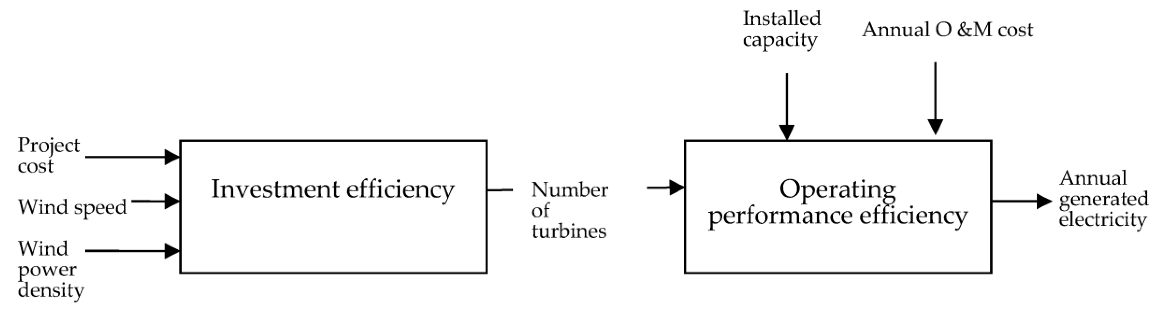
Classic single-stage DEA modeling only uses input and output information to generate the efficiency metric that represents the relationship between inputs and outputs; i.e., the maximum output given fixed inputs or the minimum input given a fixed output [26]. Each facility is regarded as a system with two sub-processes in the case of a group of WF projects: the investment and operation stage. Rather of assessing the performance of each WF project as a whole system, without recognizing its internal structure (i.e., investment and operation stage), the entire system is divided into these two sub-processes and is evaluated separately for each. Thus, the performance of the WF project involves two DEA efficiency metrics: investment stage DEA efficiency and operating stage DEA efficiency. The current study proposes a DEA with a series two-stage structure: In the first stage (investment sub-process) the contract cost of the project, wind speed and wind power density are considered inputs, while the number of turbines is the considered output. In the second stage (operation sub-process) the number of turbines (i.e., the output of the first stage) is considered to be the input along with other extra inputs such as plant operating and maintenance costs, while the electricity produced is the considered output.
3. Methods—Data Set
3.1. Series Two-Stage DEA Structure
The current study, taking into account the availability of data, employs the series two-stage DEA model to derive WF project efficiency scores in both the investment and operational stages.
The independent approach [27] is used to evaluate the WF projects (i.e., each stage is handled separately and their common feature is the outputs of the first that are inputs for the second stage), and the efficiency of each stage is separately determined. Figure 1 illustrates the DEA series two-stage structure used for the assessment of sampled WF projects. The inputs of the stage 1 are distinguished into controllable and uncontrollable as described in detail in the following subsection.
3.2. Model Building
The group of WF projects assessed in the current research includes WFs of different size, and therefore the BCC (Banker, Charnes and Cooper) model [28] was chosen to take into account the effects of the scale economies. With respect to the model orientation, input minimizing models evaluate the input decrease that could be accomplished with the current output level, while output maximization models indicate the highest possible output increase for the given input amount.
Usually, WF contractors have little to no direct control over the pre-specified number of turbines (stage 1) and therefore input orientation (i.e., BCC input-oriented model) was selected. In the operational stage 2, output optimization aims to the maximum electricity production given the inputs and, therefore, the output-oriented version of the BCC model was employed. In the case study application, the determination of to what extent the performance of WF projects could be improved in the construction phase by reducing project cost given the pre-specified project number of turbines was sought and, moreover, whether the WF operator could be effective by increasing the produced electricity from the grid-connected WFs given the number of turbines installed, capacity, and annual operating and maintenance cost.
The inputs used in DEA-based evaluation of WFs can be distinguished into discretionary (i.e., controllable) such as project cost and non-discretionary (i.e., uncontrollable) inputs, such as wind speed and wind power density. Assuming that there is a group of n WF projects, j = 1, …, n using discretionary inputs X ∈ m+ and non-discretionary inputs Z ∈ p+ to generate outputs Y ∈ k+, the following BCC (envelopment form) or variable returns to scale (VRS) input-oriented Model (3) [22,23] and output-oriented Model (4) [29] are selected to assess the investment and operational efficiency of projects, respectively:
where xij, and zlj are the ith discretionary and lth non-discretionary input, respectively, used by the jth project; yrj is rth output produced by the jth project; and denote the efficiency score of WF0 derived by the model (3) and model (4), respectively; WF0 denotes the farm under evaluation; and is intensity factor that shows the contribution of WFj in the derivation of efficiency of WF0.
The optimal solution, of Model (3), yields an investment efficiency score for the WF0. The solving process is repeated for each WF. The efficiency of WF0 deals with the WF which has inputs , and outputs , respectively. The model searches for a group of WFs created by weighting each WFj by a coefficient so that they do not generate more outputs than WF0 and minimize inputs in comparison to those of WF0. WFs for which and are deemed efficient and inefficient, respectively.
The operational efficiency of WF0 is given by , where is the optimal solution of Model (4). The model searches for a group of WFs created by weighting each WFj by a coefficient so that they do not use more inputs than WF0 and maximize outputs in comparison to those of WF0. WFs for which and are deemed efficient and inefficient, respectively.
Charnes et al. [9] developed the CCR (Charnes, Cooper and Rhodes) model that calculates the DMU’s global technical efficiency (GTE) by assuming constant scale returns (CRS). Banker et al. [28], on the other hand, proposed the BCC model, which calculates (local) pure technical efficiency (PTE) with the assumption of variable scale returns (VRS). The dual (i.e., multiplier [29]) of Model (4) can be used to estimate the returns to scale (RTS) of WFs [18]. The WFs operating at the most productive scale exhibit CRS and are scale efficient. The scale efficiency (SE) is determined by the ratio of GTE to PTE; i.e., the efficiency of the scale tests the difference between GTE and PTE [19]. The CRS version (i.e., CCR (Charnes, Cooper and Rhodes [9]) model) stems from Model (4) if the restriction is omitted. Scale inefficient WFs operate under increasing returns to scale (IRS) or decreasing returns to scale (DRS) and they should increase or decrease, respectively, their production level to become scale efficient. Table 1 summarizes all the efficiency measures used in the analysis for both input (stage 1) and output-oriented models (stage 2).
3.3. Data Set
For the purpose of the current paper study a group of thirteen Greek onshore WF projects are evaluated. In principle they are deemed homogeneous, because they use the same production technology and can therefore be compared in terms of their efficiency by means of DEA.
In the first subprocess (investment phase) project investment cost, wind speed, and wind power density are considered as inputs and the number of WTs as the output variable. Project investment cost is the total funds used during the construction period of the power facility from the design up to the start of operation [14]. Wind speed and wind power density are parameters that reflect the wind resource [21] that is provided by Nature. The wind speed is deemed as one of the most important input variables that is related to the amount of energy produced by a WT. The input to WT depends on the wind, and the wind power density (i.e., the power of the wind per unit area) is used as a proxy for the potential of site wind resources [16]. Since the wind power is determined by air volume, air speed (velocity), and air mass (density), the wind power density can be calculated by using Equation (5) [19]:
where is the wind power density, = 1.225 kg/m3 is the air density, A is the swept area (A = πr2), i.e., the area through which the rotor blades of a WT spin, is the average wind speed, and = 0.593 is a power coefficient that reflects the maximum power which can be extracted. The diameter of WT is taken from equipment technical data. It is worth noting that the average wind speed at each WF site was used to estimate the wind power density in line with previous studies [7]. A more precise estimation will require taking into account the distribution of wind speed, which is typically a Weibull distribution [7]. This was difficult to obtain in our case, because of the lack of data. The purpose of the investment phase is to arrange WTs reasonably and thus, the number of WTs is selected as the output variable [21].
The second subprocess (operating stage) deals with electricity production optimization and thus, electricity produced by each WF is set as an output variable. In line with previous DEA-based WF studies, the production factors (inputs) include installed capacity [18] and operation (including maintenance) cost [18]. In addition to these factors the current research also includes the WT number (i.e., the output of the first subprocess) [21]. The installed capacity of the WFs is obtained as the product of the number of WTs multiplied by each turbine’s nominal power [5]. The cost of operation and maintenance (O&M) is the total expense for the year. The variables used in the analysis are depicted in Table 2.
Two isotonicity tests [30], one for investment and operational process, justify the selection of input and output variables in the DEA evaluations. These tests are carried out by calculating all inter-correlations between all variables to investigate whether input increases lead to higher outputs. Tests for the two stages were passed and thus the selection of variables was justified. The 13 projects listed fulfill the criteria of the Cooper et al. thumb rule [29].
Two types of onshore WTs (WT1 and WT2) are used in the group of WFs analyzed in the current paper. The features of such WFs listed in Table 3.
The characteristics of thirteen WFs evaluated in the current paper are summarized in Table 4. Two WFs are part of autonomous systems and the rest are connected to the mainland grid. Two WFs have down-rated capacity due to grid restrictions. In more than half of the WFs the construction of a voltage rise substation is needed which increases the cost of the project.
The project investment cost and average wind speed variables used in stage 1 are taken from a previous study [13]. Wind power density and number of turbines are variables which are not considered in [13] and they are estimated in this paper. The wind power density is calculated using Equation (5) and magnitude values, as stated above. The number of turbines is estimated using data from [13] on installed capacity and nominal turbine type output. Installed capacity and annual O&M cost in stage 2 are taken from [13]. Annual electricity produced is calculated using data from [13] on annual electricity sales revenue and a tariff for each WF. The descriptive statistics of the WF project variables used are shown in Table 5.
4. Results
In the light of the results produced by the BCC input-oriented Model (3), out of the 13 projects, 5 (38%) were found to be ex-post relatively efficient; mean investment performance efficiency: 0.76. The model satisfactorily discriminates the efficient and inefficient WFs. The median investment performance efficiency was about 0.78. The efficiency score of 0.76 means that, on average, a reduction of 24% (= 1 − 0.76) of the current discretionary (i.e., controllable) input level is possible while maintaining the same level of output (Table 6). The results of the BCC output-oriented model (4) suggest that 7 (54%) of the 13 projects were found to be relatively efficient ex-post; mean operating efficiency: 0.89. The model’s discriminatory power is lower relative to stage 1, however that is a characteristic of the BCC model and, thus, the findings are deemed acceptable. Moreover, efficiency in operating phase can be improved by producing more electricity by about 12% (= (1/0.89) − 1) (Table 6). It is evident from the above findings that the construction stage is more ineffective compared to the operating stage.
One of the major drawbacks of the DEA framework is that efficiency scores are solely dependent upon the model’s input and output variables. To address this constraint, a sensitivity analysis is performed to assess the effects of input removal on the DEA efficiency scores. The efficiency scores for the different multiple-input single-output scenarios are reported in Table 7. In modified models (3′) and (3″) and models (4′) and (4″) one of the non-discretionary input and one of the input variables has been removed at a time, respectively. In all modified models at least one discretionary input and one output variable is necessary. However, the variable representing the number of turbines is not omitted because it is the variable that the two subprocesses have in common.
The average investment performance efficiency score of the original Model (3) including all the discretionary and non-discretionary inputs and the output variable is higher or equal compared to models (3′) and (3″), respectively. Removing the wind speed non-discretionary input variable results in the lowest average efficiency (0.54) in the initial Model (3). The original Model’s (4) average investment efficiency score including all the input and output variables is higher compared to models (4′) and (4″). Removing the input variable related to installed capacity in original Model (4) results in the lowest average efficiency (0.86). The results of the sensitivity analysis show that the wind power density has no effect on investment performance. The other input variables have an effect on efficiency. It is worth noticing that the installed capacity has the greater effect on operating efficiency.
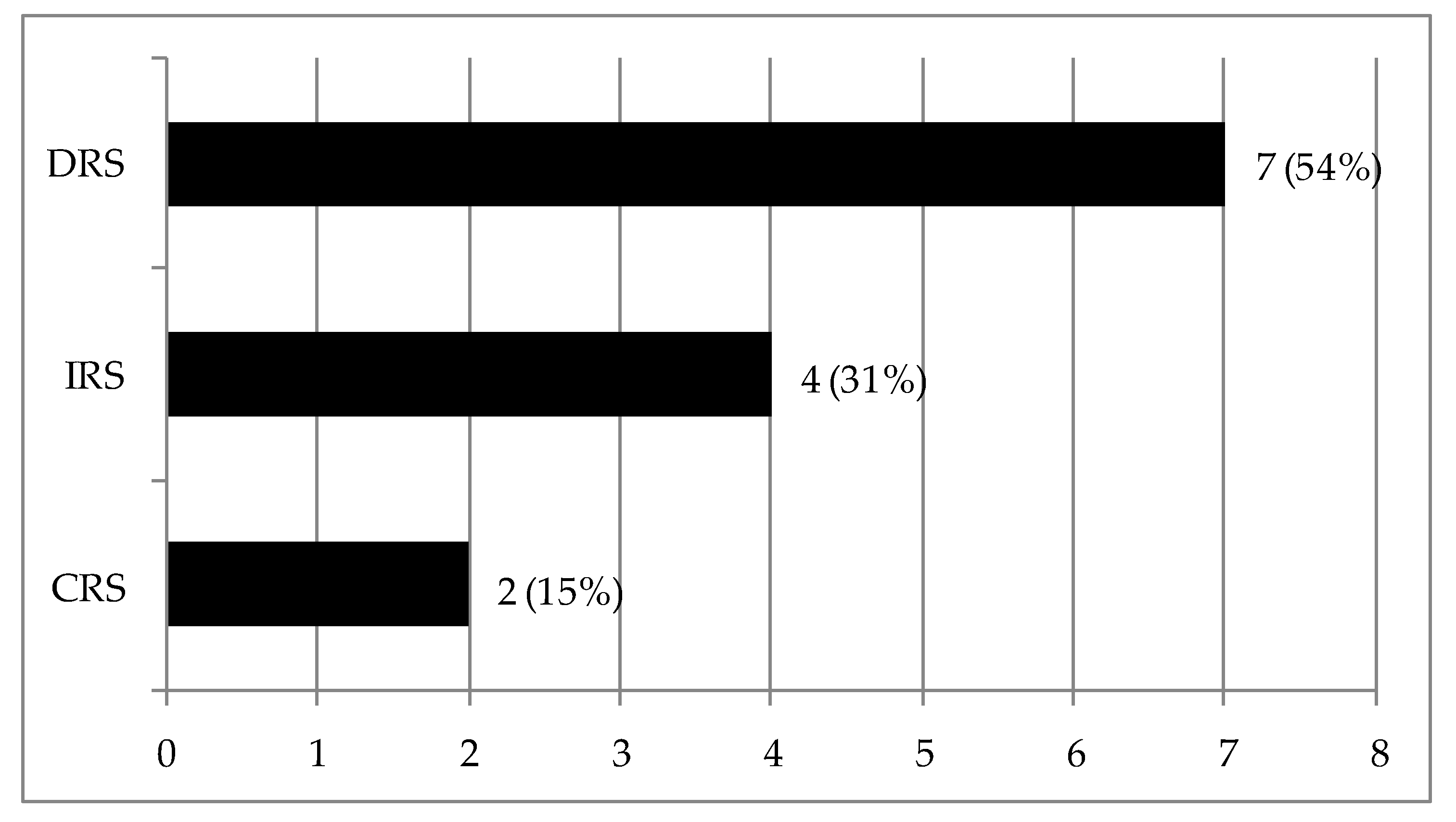
The dual BCC output-oriented model can provide information on scale efficiency and RTS. The average scale efficiency score of the sample WFs is about 0.89. There are two WFs (15% of the total) that operate at their most productive scale under CRS; WF2 and WF12 are the only scale efficient projects. As for the scale inefficient farms, four WFs (31% of the total) exhibit IRS and they should increase their size to reach the optimum production scale. Notably, the rest of WFs (54% of the total) exhibit DRS and they should decrease their size (Table 6). Figure 2 illustrates the distribution of RTS in operating performance for the sampled WFs.
In Figure 3, a so-called bubble diagram, the scale efficiency scores for operating performance and size (measured by installed capability of the WF) are plotted. Within this diagram, a circle reflects the size of a WF, with larger circles representing greater WFs. The three categories of scale (CRS, IRS, and DRS) are shown on the y-axis. From Figure 3 it is evident that large-sized WFs tend to exhibit DRS compared with the small- and medium-sized WFs that exhibit CRS and IRS.
Results of the investment performance evaluation include the WF1, WF2, WF4, WF9, and WF11 as best-in-class projects. The operating performance results include the WF1, WF2, WF3, WF7, WF8, WF11 and WF12 as the best-in-class projects. The WF1, WF2, WF11 projects are the best-in-class in both investment and operating performance. The WT2 type turbine is used by WF2 (autonomous system) and WF11 (with down-rated capacity), while the WT1 type turbine is used by WF1. In addition, the construction of a voltage rise substation is required for WF1. In the light of the sensitivity analysis results, the benchmarks of investment performance assessment in all scenarios considered are: WF1, WF2, WF9, and WF11. In the operating performance efficiency evaluation, the benchmarks for all scenarios are: WF3, WF8, WF11 and WF12. The benchmark in both dimensions of performance for all scenarios is the project WF11.
5. Conclusions
The current study adopts a series two–stage structure for the ex-post DEA-based performance assessment of a sample of 13 WF projects taking into consideration the structure of the WF projects. The data on onshore WF projects in Greece are used to illustrate the applicability and empirical usefulness of the approach being proposed. The series two-stage structure is considered superior to the traditional single-stage DEA setting because, in the case of WFs, it seeks to open the project black-box. DEA-based efficiency scores from the BCC model of input minimization are produced in the first stage of the investment project analysis using data on project cost, wind speed, and wind power density as inputs and turbine number as output. In the second stage, the operating efficiency of the WF projects is evaluated using the BCC model of output maximization using the number of turbines, installed power, and annual O&M cost as inputs and the annual electricity generated as output. The modeling approach provides project DEA-based efficiency scores for each stage that take values between zero and unity and represents how well the project performs at each stage.
The findings suggest that only five and seven of the 13 sample WF projects in stages 1 and 2, respectively, are ex-post efficient in the context of the DEA; however, only two WFs operate at the optimum production scale. It is also evident that the investment stage has a lower level of performance than the operational stage. Although the results are sample-specific, WF size appears to be related to operating efficiency. Small- and medium-sized WFs operate under CRS and IRS, while large-sized WFs operate under DRS. Moreover, in the light of the sensitivity analysis results, wind speed and WF installation capacity appear to be the factors that affect the investment performance and operational efficiency, respectively.
The derived consolidated metrics in stages 1 and 2 can serve for project managers and facility operators as an indicator for the level of achievement of the projects in the investment and operational stage, respectively. In addition, they may also be viewed as performance metrics for the project’s design and operating team.
Throughout the current study, static DEA models were used to analyze a group of WF projects from the point of view of the contractor/operator. If a long time series on WF operating data will be made available, future research can be focused on dynamic analysis and DEA can provide a dynamic evaluation of WF performance. Since the distribution of wind speed is not taken into account in the current research this can be seen as a limitation of the study that can be addressed by using high-frequency data in future research.
Funding
This research received no external funding.
Acknowledgments
The author gratefully acknowledges the constructive comments of four referees on an earlier version of the manuscript.
Conflicts of Interest
The author declares no conflict of interest.
References
- Chen, Z. Wind power in modern power systems. J. Mod. Power Syst. Clean Energy 2013, 1, 2–13. [Google Scholar] [CrossRef] [Green Version]
- Iribarren, D.; Vázquez-Rowe, I.; Rugani, B.; Benetto, E. On the feasibility of using emergy analysis as a source of benchmarking criteria through data envelopment analysis: A case study for wind energy. Energy 2014, 67, 527–537. [Google Scholar] [CrossRef]
- Wind Europe. Wind Energy in Europe in 2019: Trends and Statistics; Wind Europe: Brussels, Belgium, 2020. [Google Scholar]
- Hwangbo, H.; Johnson, A.; Ding, Y. A production economics analysis for quantifying the efficiency of wind turbines. Wind Energy 2017, 20, 1501–1513. [Google Scholar] [CrossRef]
- Aigner, D.J.; Lovell, C.A.K.; Schmidt, P.J. Formulation and estimation of stochastic frontier production function models. J. Econ. 1977, 6, 21–37. [Google Scholar] [CrossRef]
- Meeusen, W.; van den Broeck, J. Efficiency Estimation from Cobb-Douglas Production Functions with Composed Error. Int. Econ. Rev. 1977, 18, 435. [Google Scholar] [CrossRef]
- Iglesias, G.; Castellanos, P.; Seijas, A.; Castellanos-García, P. Measurement of productive efficiency with frontier methods: A case study for wind farms. Energy Econ. 2010, 32, 1199–1208. [Google Scholar] [CrossRef]
- Jradi, S.; Ruggiero, J. Stochastic data envelopment analysis: A quantile regression approach to estimate the production frontier. Eur. J. Oper. Res. 2019, 278, 385–393. [Google Scholar] [CrossRef]
- Charnes, A.; Cooper, W.W.; Rhodes, E. Measuring the efficiency of decision making units. Eur. J. Oper. Res. 1978, 2, 429–444. [Google Scholar] [CrossRef]
- Tsolas, I.E. Benchmarking Engineering, Procurement and Construction (EPC) Power Plant Projects by Means of Series Two-Stage DEA. Electricity 2020, 1, 1. [Google Scholar] [CrossRef]
- Kao, C. Network data envelopment analysis: A review. Eur. J. Oper. Res. 2014, 239, 1–16. [Google Scholar] [CrossRef]
- Sarıca, K.; Or, I.; Sarica, K. Efficiency assessment of Turkish power plants using data envelopment analysis. Energy 2007, 32, 1484–1499. [Google Scholar] [CrossRef]
- Champlilomatis, P. Benchmarking of Renewable Energy Source Projects. Master’s Thesis, Hellenic Open University, Patras, Greece, 2013. (In Greek). [Google Scholar]
- Kim, K.-T.; Lee, D.-J.; Park, S.-J.; Zhang, Y.; Sultanov, A. Measuring the efficiency of the investment for renewable energy in Korea using data envelopment analysis. Renew. Sustain. Energy Rev. 2015, 47, 694–702. [Google Scholar] [CrossRef]
- Akbari, N.; Jones, D.; Treloar, R. A cross-European efficiency assessment of offshore wind farms: A DEA approach. Renew. Energy 2019, 151, 1186–1195. [Google Scholar] [CrossRef]
- Rodríguez, X.P.; Regueiro, R.M.; Doldán, X.R. Analysis of productivity in the Spanish wind industry. Renew. Sustain. Energy Rev. 2020, 118, 109573. [Google Scholar] [CrossRef]
- Coelli, T.; Rao, D.S.P.; Battese, G.E. An Introduction to Efficiency and Productivity Analysis; Kluwer Academic Publishers: Boston, MA, USA, 1999. [Google Scholar]
- Wu, Y.; Hu, Y.; Xiao, X.; Mao, C. Efficiency assessment of wind farms in China using two-stage data envelopment analysis. Energy Convers. Manag. 2016, 123, 46–55. [Google Scholar] [CrossRef]
- Saglam, U. A two-stage data envelopment analysis model for efficiency assessments of 39 state’s wind power in the United States. Energy Convers. Manag. 2017, 146, 52–67. [Google Scholar] [CrossRef]
- Ederer, N. Evaluating capital and operating cost efficiency of offshore wind farms: A DEA approach. Renew. Sustain. Energy Rev. 2015, 42, 1034–1046. [Google Scholar] [CrossRef]
- Niu, D.; Song, Z.; Xiao, X.; Wang, Y. Analysis of wind turbine micrositing efficiency: An application of two-subprocess data envelopment analysis method. J. Clean. Prod. 2018, 170, 193–204. [Google Scholar] [CrossRef]
- Banker, R.D.; Morey, R.C. Efficiency Analysis for Exogenously Fixed Inputs and Outputs. Oper. Res. 1986, 34, 513–521. [Google Scholar] [CrossRef]
- Wang, D. Benchmarking the Performance of Solar Installers and Rooftop Photovoltaic Installations in California. Sustainability 2017, 9, 1403. [Google Scholar] [CrossRef] [Green Version]
- Saglam, U. A two-stage performance assessment of utility-scale wind farms in Texas using data envelopment analysis and Tobit models. J. Clean. Prod. 2018, 201, 580–598. [Google Scholar] [CrossRef]
- Iribarren, D.; Martín-Gamboa, M.; Dufour, J. Environmental benchmarking of wind farms according to their operational performance. Energy 2013, 61, 589–597. [Google Scholar] [CrossRef]
- Farrell, M.J. The Measurement of Productive Efficiency. J. R. Stat. Soc. Ser. A (Gen.) 1957, 120, 253. [Google Scholar] [CrossRef]
- Koronakos, G. A Taxonomy and Review of the Network Data Envelopment Analysis Literature. In Machine Learning Paradigms; Tsihrintzis, G., Virvou, M., Sakkopoulos, E., Jain, L., Eds.; Springer: Cham, Switzerland, 2019; Volume 1, pp. 255–311. [Google Scholar]
- Banker, R.D.; Charnes, A.; Cooper, W.W. Some Models for Estimating Technical and Scale Inefficiencies in Data Envelopment Analysis. Manag. Sci. 1984, 30, 1078–1092. [Google Scholar] [CrossRef] [Green Version]
- Cooper, W.W.; Seiford, L.M.; Tone, T. Data Envelopment Analysis: A Comprehensive Text with Models, Applications, References and DEA-Solver Software; Springer Science + Business Media, Inc.: New York, NY, USA, 2007. [Google Scholar]
- Mostafa, M.M. Modeling the competitive market efficiency of Egyptian companies: A probabilistic neural network analysis. Expert Syst. Appl. 2009, 36, 8839–8848. [Google Scholar] [CrossRef]
Figure 1.
Investment and operating performance efficiency of wind farm WF sampled projects.

Figure 2.
Summary of RTS data of WFs—Stage 2 (Operating efficiency).

Figure 3.
Scale of operation. Stage 2 (Operating efficiency).


Table 1.
Summary of the efficiency calculations.
| Model | Input-Oriented Model—Stage 1 | Output-Oriented Model—Stage 2 | Efficiency Definition |
|---|---|---|---|
| BCC input oriented efficiency (PTEin) | Scalar derived from Model (3) | ||
| CCR output oriented efficiency (GTEout) | Scalar derived from a modified Model (4) without the restriction | ||
| BCC output oriented efficiency (PTEout) | Reciprocal of scalar derived from Model (4) | ||
| Scale output oriented efficiency (SEout) | SEout = GTEout/PTEout |
Table 2.
Variable descriptions.
| Variable | Definition | Units | Source |
|---|---|---|---|
| Project cost | Estimated cost to complete the project | 106 Euros | [13] |
| Wind speed | Speed (velocity) of air | m/s | [13] |
| Wind power density | Wind power available per square meter of swept area of a turbine | W/m2 | This study |
| Number of wind turbines | The number of wind turbines | 1 | This study |
| Installed capacity | Facility capacity | MW | [13] |
| Operating and maintenance cost | Estimated cost of annual operating and maintenance cost | 106 Euros | [13] |
| Power generation | Estimated annual generated electricity | MWh | This study |
Table 3.
Specification of the wind turbines.
| Features | WT1 | WT2 |
|---|---|---|
| Rotor diameter, m | 90 | 52 |
| Area swept, m2 | 6362 | 2124 |
| Number of blades | 3 | 3 |
| Wind speed cut-in, m/s | 4 | 4 |
| Wind speed rated, m/s | 15 | 14 |
| Wind speed cut-out, m/s | 25 | 25 |
| Nominal output, kW | 3000 | 850 |
| Installation | Onshore | Onshore |
Table 4.
Summary of WF characteristics.
| Project No. | Wind Turbine Type | Autonomous System | Down-Rated Capacity | Voltage Rise Substation Construction |
|---|---|---|---|---|
| WF1 | WT1 | ✓ | ||
| WF2 | WT2 | ✓ | ||
| WF3 | WT1 | ✓ | ||
| WF4 | WT1 | ✓ | ||
| WF5 | WT1 | ✓ | ||
| WF6 | WT1 | ✓ | ||
| WF7 | WT1 | ✓ | ||
| WF8 | WT1 | ✓ | ||
| WF9 | WT1 | ✓ | ✓ | |
| WF10 | WT1 | |||
| WF11 | WT2 | |||
| WF12 | WT1 | |||
| WF13 | WT2 | ✓ |
Table 5.
WF projects: Descriptive statistics.
| Descriptive Statistics | Project Cost (106 Euros) | Wind Speed (m/s) | Wind Power Density (W/m2) | Number of Wind Turbines | Installed Capacity (MW) | Annual Operating and Maintenance Cost (106 Euros) | Power Generation (103 MWh) |
|---|---|---|---|---|---|---|---|
| Mean | 20.78 | 7.57 | 3.25 | 7.15 | 17.88 | 0.55 | 38.10 |
| Standard deviation | 12.07 | 1.11 | 1.29 | 3.29 | 10.97 | 0.32 | 20.57 |
| Median | 25.15 | 7.47 | 3.16 | 8.00 | 18.00 | 0.49 | 38.39 |
| Min | 2.86 | 5.63 | 1.65 | 3.00 | 2.55 | 0.09 | 5.77 |
| Max | 34.66 | 9.37 | 5.83 | 12.00 | 36.00 | 1.12 | 67.20 |
Table 6.
WF project efficiency measures for investment and operating phase and descriptive statistics.
Table 6.
WF project efficiency measures for investment and operating phase and descriptive statistics.
| Project No. | Investment Phase | Operating Phase | ||
|---|---|---|---|---|
| Investment Performance (%) | Operating Efficiency (%) | Scale Efficiency (%) | RTS | |
| WF1 | 100.00 | 100.00 | 67.42 | DRS |
| WF2 | 100.00 | 100.00 | 100.00 | CRS |
| WF3 | 75.07 | 100.00 | 77.08 | DRS |
| WF4 | 100.00 | 75.99 | 98.91 | IRS |
| WF5 | 85.01 | 77.66 | 84.10 | DRS |
| WF6 | 78.04 | 78.15 | 99.46 | IRS |
| WF7 | 67.52 | 100.00 | 74.50 | DRS |
| WF8 | 35.19 | 100.00 | 99.30 | DRS |
| WF9 | 100.00 | 66.64 | 81.56 | DRS |
| WF10 | 46.03 | 87.31 | 85.96 | DRS |
| WF11 | 100.00 | 100.00 | 94.37 | IRS |
| WF12 | 31.42 | 100.00 | 100.00 | CRS |
| WF13 | 66.43 | 74.59 | 92.36 | IRS |
| Mean | 75.75 | 89.26 | 88.85 | |
| Standard deviation | 25.30 | 12.82 | 11.19 | |
| Median | 78.04 | 100.00 | 92.36 | |
| Min | 31.42 | 66.64 | 67.42 | |
| Max | 100.00 | 100.00 | 100.00 | |
Returns to scale; CRS: Constant returns to scale; IRS: Increasing returns to scale; DRS: Decreasing returns to scale.
Table 7.
Sensitivity analysis results.
| Variables | Investment Performance | Operating Efficiency | ||||
|---|---|---|---|---|---|---|
| Original Model (Model (3)) | Modified Model (3′) | Modified Model (3″) | Original Model (Model (4)) | Modified Model (4′) | Modified Model (4″) | |
| Project cost | ✓ | ✓ | ✓ | |||
| Wind speed | ✓ | ✓ | ||||
| Wind power density | ✓ | ✓ | ||||
| Number of turbines | ✓ | ✓ | ✓ | ✓ | ✓ | ✓ |
| Installed capacity | ✓ | ✓ | ||||
| Annual O&M cost | ✓ | ✓ | ||||
| Annual generated electricity | ✓ | ✓ | ✓ | |||
| Average efficiency score (%) | 75.75 | 53.90 | 75.75 | 89.26 | 86.11 | 87.29 |
© 2020 by the author. Licensee MDPI, Basel, Switzerland. This article is an open access article distributed under the terms and conditions of the Creative Commons Attribution (CC BY) license (http://creativecommons.org/licenses/by/4.0/).
Share and Cite
MDPI and ACS Style
Tsolas, I.E. Benchmarking Wind Farm Projects by Means of Series Two-Stage DEA. Clean Technol. 2020, 2, 365-376. https://0-doi-org.brum.beds.ac.uk/10.3390/cleantechnol2030022
AMA Style
Tsolas IE. Benchmarking Wind Farm Projects by Means of Series Two-Stage DEA. Clean Technologies. 2020; 2(3):365-376. https://0-doi-org.brum.beds.ac.uk/10.3390/cleantechnol2030022
Chicago/Turabian StyleTsolas, Ioannis E. 2020. "Benchmarking Wind Farm Projects by Means of Series Two-Stage DEA" Clean Technologies 2, no. 3: 365-376. https://0-doi-org.brum.beds.ac.uk/10.3390/cleantechnol2030022