On the Tree Gauge in Magnetostatics

Abstract

We recall the classical tree-cotree technique in magnetostatics. (1) We extend it in the frame of high-order finite elements in general domains. (2) We focus on its connection with the question of the invertibility of the final algebraic system arising from a high-order edge finite element discretization of the magnetostatic problem formulated in terms of the magnetic vector potential. With the same purpose of invertibility, we analyse another classically used condition, the Coulomb gauge. (3) We conclude by underlying that the two gauges can be naturally considered in a high order framework without any restriction on the topology of the domain.

1. Introduction

We extend, in an easy way, the classical tree-cotree technique in the frame of high-order finite elements (FEs). We focus on magnetostatics as it represents a significative problem where this technique is usually applied. Particular attention is given to the magnetic vector potential formulation of such a problem. This problem admits infinite solutions hence its discretization by Whitney edge FEs yields to a singular algebraic system.

The techniques that are generally adopted in magnetostatics to eliminate the matrix nullspace are described in two seminal works, one by Albanese and Rubinacci [1] and the other by Cendes and Manges [2]. Albanese and Rubinacci showed that one converts the singular systems, resulting from low-order edge-based discretizations of magnetostatic problems, into nonsingular ones by setting to zero the vector potential circulations on a spanning tree edges of the FE mesh graph. Manges and Cendes underlined the relation between the tree-cotree approach proposed by Albanese and Rubinacci and the enforcement in a weak sense of the Coulomb gauge. The tree-cotree technique was then used for example in [3] to reduce the number of unknowns of a three-dimensional magnetostatic problem or in [4] to solve the eddy-current problem in a multiply connected region. It has led to several variants, see an overview in [5]. The tree-cotree decomposition of the unknowns in two-dimensional applications has been also considered for face elements in [6]. Indeed, in two dimensions, the face element basis functions are obtained from the edge element ones by a rotation of 90 degrees. However, in all the previous works, only the lowest order finite element discretisation is considered, which simplifies the identification of the degrees of freedom (dofs) with mesh edges. Indeed, with classical edge FEs, dofs are the circulations of the approximated vector field along the edges of the FE mesh [7]. Hence, tree-cotree techniques are perfectly adapted to this type of discretizations since there is a one-to-one correspondence between edges, listed in the tree or cotree sets, and dofs.

In a high order FE discretization of the same problem, the dofs introduced in [8], the so-called weights, have again a physical signification. For edge discretizations, they have the meaning of circulations on suitable edges of a fictitious refinement of the FE mesh. This fact allows us to rely in a very natural way on tree-cotree techniques. These new dofs were born from using the same geometrical approach, proposed by Whitney [9] to construct low order polynomial representations of differential forms, on a finer simplicial complex of the computational domain mesh. These weights do coincide with Whitney edge FE dofs in the low-order case.

In these pages, by relying on linear algebra, we analyse the fundamental work accomplished in the 90 s on tree-cotree techniques and show that it is still in actuality in the high order case when fields are reconstructed in the discrete space by using their weights. Further, the interest of the analysis presented, for the weights, in these pages is to underline that the tree-cotree approach can be adopted within any high order FE approach where it is possible to state a clear correspondence of dofs with geometrical objects creating a graph.

We thus start by considering an open bounded connected polyhedral domain $\mathsf{\Omega }\subset {\mathbb{R}}^3$ with boundary $\partial \mathsf{\Omega }$. We indicate by ${(\partial \mathsf{\Omega })}_j$, for $j=0,\dots ,p$, the connected components of $\partial \mathsf{\Omega }$ (in particular, ${(\partial \mathsf{\Omega })}_0$ is the external one). We denote by g the number of independent non-bounding cycles in $\mathsf{\Omega }$. Note that $b_1\left(\mathsf{\Omega }\right)=g$ and $b_2\left(\mathsf{\Omega }\right)=p$ are, respectively, the first and the second Betti numbers of $\mathsf{\Omega }$ (see, e.g., [10]). For a domain $\mathsf{\Omega }\subset {\mathbb{R}}^3$, the 0th Betti number $b_0\left(\mathsf{\Omega }\right)$ is equal to the number of connected components of $\mathsf{\Omega }$. If $\mathsf{\Omega }$ is connected, as assumed in these pages, then $b_0\left(\mathsf{\Omega }\right)=1$. The third Betti number $b_3\left(\mathsf{\Omega }\right)=0$ in the present case. Betti numbers describe the topology of $\mathsf{\Omega }$ and provide a way of computing its Euler-Poincaré characteristic as the number $\chi \left(\mathsf{\Omega }\right)=b_0-b_1+b_2-b_3$. We introduce the space of the magnetic harmonic vector fields, that is

$${\mathcal{H}}_{\mu }(\mathrm{m};\mathsf{\Omega })=\{\mathbf{w}\in {\left(L^2\left(\mathsf{\Omega }\right)\right)}^3,\mathbf{curl}\mathbf{w}=\mathbf{0},\mathrm{div}\left(\mu \mathbf{w}\right)=0,\mu \mathbf{w}·{\mathbf{n}}_{\partial \mathsf{\Omega }}=0\mathrm{on}\partial \mathsf{\Omega }\}.$$

We recall that $\dim \left({\mathcal{H}}_{\mu }(\mathrm{m};\mathsf{\Omega })\right)=g$ $(=b_1\left(\mathsf{\Omega }\right))$. The magnetostatic problem in its most basic form reads: find the magnetic induction field $\mathbf{B}$ due to prescribed compatible currents $\mathbf{J}$ and defined by the field equations and conditions

$$\begin{array}{cc}\hfill \mathbf{curl}\left({\mu }^{-1}\mathbf{B}\right)=\mathbf{J},& \mathrm{in}\mathsf{\Omega },\hfill \\ \hfill \mathrm{div}\mathbf{B}=0,& \mathrm{in}\mathsf{\Omega },\hfill \\ \hfill \mathbf{B}·{\mathbf{n}}_{|\partial \mathsf{\Omega }}=0,& \mathrm{on}\partial \mathsf{\Omega },\hfill \\ \hfill {\int }_{\mathsf{\Omega }}{\mu }^{-1}\mathbf{B}·\mathbf{w}=0,& \forall \mathbf{w}\in {\mathcal{H}}_{\mu }(\mathrm{m};\mathsf{\Omega }).\hfill \end{array}$$

(1)

Here above, ${\mathbf{n}}_{|\partial \mathsf{\Omega }}$ is the outward going unit normal to $\partial \mathsf{\Omega }$ and $\mu$ the magnetic permeability of the material contained in $\mathsf{\Omega }$. It is assumed that $\mu \in L^{\infty }\left(\mathsf{\Omega }\right)$ is symmetric and positive definite, bounded from below, namely, $\mu \ge {\mu }_0>0$ for a real number ${\mu }_0$ (that coincides with the magnetic permeability of the air). The last condition of $L^2$-orthogonality to the space ${\mathcal{H}}_{\mu }(\mathrm{m};\mathsf{\Omega })$ is of key importance to guarantee the solution uniqueness. Indeed, when $\mathbf{J}=\mathbf{0}$, the first three equations in (1) give ${\mu }^{-1}\mathbf{B}\in {\mathcal{H}}_{\mu }(\mathrm{m};\mathsf{\Omega })$ that, together with the last condition, yields ${\mu }^{-1}\mathbf{B}=\mathbf{0}$, that means $\mathbf{B}=\mathbf{0}$, due to the properties of $\mu$ (see more details in [11]). For compatible currents, we mean $\mathbf{J}$ such that $\mathrm{div}\mathbf{J}=0$ in $\mathsf{\Omega }$ and ${\int }_{{(\partial \mathsf{\Omega })}_j}\mathbf{J}·{\mathbf{n}}_{|\partial \mathsf{\Omega }}=0$, for any jth (out of $p+1$) connected component ${(\partial \mathsf{\Omega })}_j$ of $\partial \mathsf{\Omega }$.

The paper layout is as follows. In Section 2, we reformulate problem (1) in terms of the magnetic vector potential and its weak formulation. We thus define the high-order FE approximation space and write the discrete problem together with its matrix form in Section 3. In Section 4 we present the tree-cotree approach and the analysis of the linear system to solve in the block form dictated by the tree. Section 5 is dedicated to the imposition of a discrete Coulomb-like gauge. We briefly discuss in Section 6 about the other formulation of the magnetostatic problem and on its connection with the tree-cotree approach. We conclude in Section 7 by analysing differences and similarities between the presented gauges.

2. The Magnetic Vector Potential Problem

A way to exactly satisfy the solenoidality condition $\mathrm{div}\mathbf{B}=0$ on the magnetic induction field $\mathbf{B}$ is to represent $\mathbf{B}$ in terms of a vector potential, namely a vector $\mathbf{A}$ such that $\mathbf{B}=\mathbf{curl}\mathbf{A}$. This magnetic potential $\mathbf{A}$ is not uniquely defined as the vector $\tilde{\mathbf{A}}=\mathbf{A}+\mathbf{grad}V$, for V a scalar function, still verifies $\mathbf{B}=\mathbf{curl}\tilde{\mathbf{A}}$. A classical way to ensure the uniqueness of $\mathbf{A}$ is to prescribe a gauge condition on $\mathbf{A}$, e.g., the Coulomb gauge $\mathrm{div}\mathbf{A}=0$. We introduce the space of the electric harmonic vector fields, as

$$\mathcal{H}(\mathrm{e};\mathsf{\Omega })=\{\mathbf{w}\in {\left(L^2\left(\mathsf{\Omega }\right)\right)}^3,\mathbf{curl}\mathbf{w}=\mathbf{0},\mathrm{div}\mathbf{w}=0,\mathbf{w}\times {\mathbf{n}}_{\partial \mathsf{\Omega }}=\mathbf{0}\mathrm{on}\partial \mathsf{\Omega }\}.$$

It holds that $\dim \left(\mathcal{H}\right(\mathrm{e};\mathsf{\Omega }\left)\right)=p$ $(=b_2\left(\mathsf{\Omega }\right))$. The magnetostatic problem (1) thus reads: given a compatible $\mathbf{J}$, find a vector $\mathbf{A}$ satisfying the field equations (as stated in, e.g., [12])

$$\begin{array}{cc}\hfill \mathbf{curl}{\mu }^{-1}\mathbf{curl}\mathbf{A}& =\mathbf{J}\mathrm{in}\mathsf{\Omega },\hfill \\ \hfill \mathrm{div}\mathbf{A}& =0\mathrm{in}\mathsf{\Omega },\hfill \\ \hfill \mathbf{A}\times {\mathbf{n}}_{|\partial \mathsf{\Omega }}& =\mathbf{0}\mathrm{on}\partial \mathsf{\Omega },\hfill \\ \hfill {\int }_{{(\partial \mathsf{\Omega })}_j}\mathbf{A}·{\mathbf{n}}_{\partial \mathsf{\Omega }}& =0\forall j=0,\dots ,p.\hfill \end{array}$$

(2)

We remark that from the boundary condition $\mathbf{A}\times {\mathbf{n}}_{|\partial \mathsf{\Omega }}=\mathbf{0}$ it follows $\mathbf{curl}\mathbf{A}·{\mathbf{n}}_{|\partial \mathsf{\Omega }}=0$ hence $\mathbf{B}·{\mathbf{n}}_{|\partial \mathsf{\Omega }}=0$. It is possible to show (see again [11]) that $\mathbf{grad}{z}_j\in \mathcal{H}(\mathrm{e};\mathsf{\Omega })$ for each function $z_j\in H^1\left(\mathsf{\Omega }\right)$ that is solution of $\mathrm{div}\mathbf{grad}{z}_j=0$ in $\mathsf{\Omega }$, with boundary conditions ${\left(z_j\right)}_{{|(\partial \mathsf{\Omega })}_i}={\delta }_{ij}$, for $i,j=0,\dots ,p$ (here ${\delta }_{..}$ is the Kronecker symbol, namely ${\delta }_{ij}$ takes the value 1 if $i=j$ and 0 otherwise). If $\mathbf{J}=\mathbf{0}$, we have $\mathbf{curl}\mathbf{A}=\mathbf{0}$. If $\mathrm{div}\mathbf{A}=0$ and ${\int }_{\mathsf{\Omega }}\mathbf{A}·\mathbf{grad}{z}_j=0$ then ${\int }_{{(\partial \mathsf{\Omega })}_j}\mathbf{A}·{\mathbf{n}}_{\partial \mathsf{\Omega }}=0$, for each $j=0,\dots ,p$.

In view of using FEs, we need to rewrite problem (2) in weak form. We multiply the first equation of (2) by a test function $\mathbf{v}\in H_0\left(\mathbf{curl};\mathsf{\Omega }\right)$ where $H_0\left(\mathbf{curl};\mathsf{\Omega }\right)=\{\mathbf{u}\in {\left(L^2\left(\mathsf{\Omega }\right)\right)}^3,\mathbf{curl}\mathbf{u}\in {\left(L^2\left(\mathsf{\Omega }\right)\right)}^3,\mathbf{u}\times {\mathbf{n}}_{|\partial \mathsf{\Omega }}=0\}$. We then integrate by parts over $\mathsf{\Omega }$ to obtain

$${\int }_{\mathsf{\Omega }}{\mu }^{-1}\mathbf{curl}\mathbf{A}·\mathbf{curl}\mathbf{v}={\int }_{\mathsf{\Omega }}\mathbf{J}·\mathbf{v},\forall \mathbf{v}\in H_0\left(\mathbf{curl};\mathsf{\Omega }\right).$$

(3)

The condition $\mathrm{div}\mathbf{A}=0$ yields the following characterisation for $\mathbf{A}$ in $\mathsf{\Omega }$:

$${\int }_{\mathsf{\Omega }}\mathrm{div}\mathbf{A}\phi =0,\forall \phi \in {\mathcal{C}}_c^{\infty }\left(\mathsf{\Omega }\right),$$

(4)

being ${\mathcal{C}}_c^{\infty }\left(\mathsf{\Omega }\right)$ the space of smooth functions with compact support in $\mathsf{\Omega }$. By integration by parts and applying a density argument, we can write

$${\int }_{\mathsf{\Omega }}\mathbf{A}·\mathbf{grad}\phi =0,\forall \phi \in H_0^1\left(\mathsf{\Omega }\right),$$

(5)

and (5) yields $\mathrm{div}\mathbf{A}=0$ in $\mathsf{\Omega }$ (in the sense of distributions). When $p>0$, the second and fourth equations in problem (2) can be imposed by using (5) with $\phi \in H_{*}^1\left(\mathsf{\Omega }\right)=\{\phi \in H^1\left(\mathsf{\Omega }\right),{\phi }_{{|(\partial \mathsf{\Omega })}_j}={\mathbf{c}}_j,\forall j=0,\dots ,p\}$ where $\mathbf{c}\in {\mathbb{R}}^{p+1}$ is a constant vector. In fact, taking $z_i\in H_{*}^1\left(\mathsf{\Omega }\right)$, with ${\mathbf{c}}_j={\delta }_{ij}$ for all $i,j=0,\dots ,p$, we have

$$0={\int }_{\mathsf{\Omega }}\mathbf{A}·\mathbf{grad}{z}_i=-{\int }_{\mathsf{\Omega }}\mathrm{div}\mathbf{A}{z}_i+{\int }_{\partial \mathsf{\Omega }}\mathbf{A}·{\mathbf{n}}_{\partial \mathsf{\Omega }}{z}_i={\int }_{{(\partial \mathsf{\Omega })}_i}\mathbf{A}·{\mathbf{n}}_{\partial \mathsf{\Omega }}.$$

We thus look for $\mathbf{A}\in H_0\left(\mathbf{curl};\mathsf{\Omega }\right)$ such that (3) holds together with the condition

$${\int }_{\mathsf{\Omega }}\mathbf{A}·\mathbf{grad}\phi =0,\forall \phi \in H_{*}^1\left(\mathsf{\Omega }\right).$$

(6)

3. The Discrete Problem and Its Matrix Form

Let ${\tau }_h=(V,E,F,T)$ be a simplicial triangulation over $\mathsf{\Omega }$ and ${\mathsf{\Omega }}_h={\cup }_{t\in T}t$. Even if ${\tau }_h$ is a simplicial triangulation of $\mathsf{\Omega }$, the topological properties computed on ${\mathsf{\Omega }}_h$ are the same as those of $\mathsf{\Omega }$. For $\mathsf{\Omega }$ connected, with g loops and p cavities, the Euler-Poincaré characteristics $\chi \left(\mathsf{\Omega }\right)$ and $\chi \left({\mathsf{\Omega }}_h\right)$ are equal and we have

$$(\chi \left(\mathsf{\Omega }\right)=b_0-b_1+b_2-b_3=)1-g+p=n_V-n_E+n_F-n_T(=\chi \left({\mathsf{\Omega }}_h\right))$$

where $n_V$, $n_E$, $n_F$, $n_T$ are, respectively, the cardinalities of the sets of vertices V, edges E, faces F and tetrahedra T of the mesh ${\tau }_h$. Given a simplicial mesh ${\tau }_h$ over $\overline{\mathsf{\Omega }}$, we denote by $W_{r+1}^k={\mathcal{P}}_{r+1}^{-}{\mathsf{\Lambda }}^k\left({\tau }_h\right)$ the set of Whitney differential k-forms of polynomial degree $r+1$, where $k\in \{0,1,2,3\}$ is the order of the form (see [13] for more details on the properties of these spaces). It is a compact notation to indicate space of polynomial functions which are well-known in finite elements. Indeed, for $k=0$, we have $W_{r+1}^0=L_{r+1}$, the space of continuous, piecewise polynomials of degree $r+1$; for $k=1$, we obtain $W_{r+1}^1=N_{r+1}$ the first family of Nédélec edge element functions of degree $r+1$; for $k=2$, we get $W_{r+1}^2=R{T}_{r+1}$ the space of Raviart-Thomas functions of degree $r+1$; for $k=3$, we find $W_{r+1}^3=P_r$ discontinuous piecewise polynomials of degree r. The spaces $W_{r+1}^k$ are connected in a complex by linear operators which can be represented by suitable matrices, namely G ($k=0$), R ($k=1$), D ($k=2$) respectively, once a set of unisolvent dofs and consequently a basis in each space $W_{r+1}^k$ have been fixed. Note that the entries of these matrices are $0,\pm 1$, only for few bases of these spaces $W_{r+1}^k$ associated with dofs chosen as, for example, the weights of a physical field, intended as a differential k-form, on chains of k-simplices of the high-order FE mesh.

For $r=0$, the dimension of the space $W_1^k$ coincides with the number of k-simplices in the mesh, indeed $\dim L_1=n_V$, $\dim N_1=n_E$, $\dim R{T}_1=n_F$ and $\dim P_0=n_T$. Moreover, the matrices G, R, D are, resp., the edge-to-node, face-to-edge and tetrahedron-to-face connectivity matrices taking also into account respective orientations. Dofs for fields in $W_1^k$ are, respectively, their values at the mesh nodes ($k=0$), their circulations along the edges ($k=1$), their fluxes across the mesh faces ($k=2$) and their densities at the mesh tetrahedra ($k=3$).

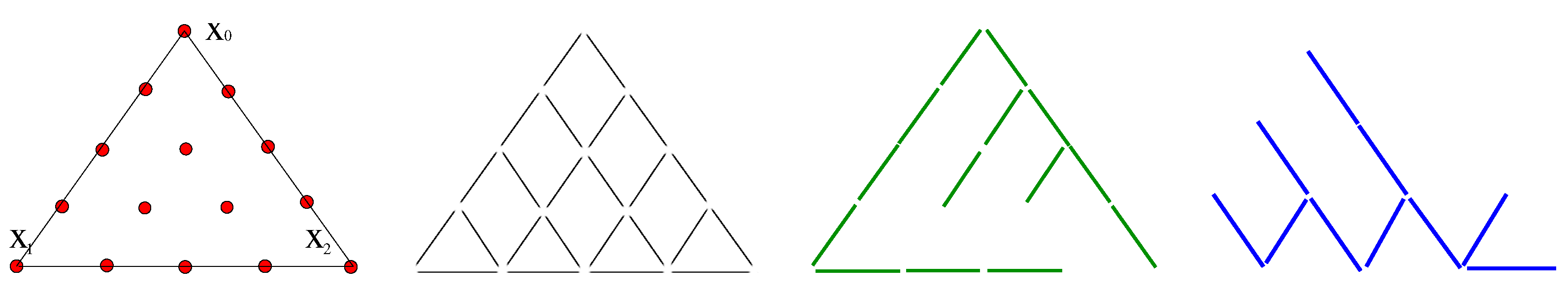
For $r>0$, as explained in [8], by connecting the nodes of the principal lattice of degree $r+1$ in a n-simplex $t\in T$, we obtain a number of small n-simplices that are $1/(r+1)$-homothetic to t. The small k-simplices, $0\le k<n$, are all the k-simplices that compose the boundary of the small n-simplices. Any small k-simplex is denoted by a couple $\{\mathbf{\alpha },s\}$, with s a k-simplex of ${\tau }_h$ and $\mathbf{\alpha }$ is a multi-integer $({\alpha }_0,\cdots ,{\alpha }_n)$ with ${\sum }_{i=0}^n{\alpha }_i=r$, ${\alpha }_i\in \mathbb{Z}$ and ${\alpha }_i\ge 0$. By relying on the last two pictures on the right of Figure 1, we give an example of small edges $\{\mathbf{\alpha },s\}$ with $r+1=4$. In the first of these two pictures, the three small edges lying at the interior of T are, respectively, $\{(1,1,1),[x_0,x_1]\}$ (left), $\{(1,0,2),[x_0,x_1]\}$ (right), $\{(2,0,1),[x_0,x_1]\}$ (top). In the last picture, the small edge lying on the boundary of T is $\{(0,0,3),[x_1,x_2]\}$. The term active is to indicate all couples $\{\mathbf{\alpha },s\}$ such that the function ${\lambda }^{\mathbf{\alpha }}{\mathbf{w}}^s$ belongs to a basis of $W_{r+1}^k$, where ${\lambda }^{\mathbf{\alpha }}={\lambda }_0^{{\alpha }_0}{\lambda }_1^{{\alpha }_1}\cdots {\lambda }_n^{{\alpha }_n}$ and ${\mathbf{w}}^s\in W_1^k$. Indeed, by considering all possible multi-indices $\mathbf{\alpha }$ in the couples $\{\mathbf{\alpha },s\}$, one generates more functions ${\lambda }^{\mathbf{\alpha }}{\mathbf{w}}^s$ than necessary. The dimension of the space $W_{r+1}^k$ coincides with the number of active small k-simplices in the mesh. The small k-simplices were born to define a set of unisolvent dofs, the weights ${\int }_{\{\mathbf{\alpha },s\}}u$, for functions $u\in W_{r+1}^k\left(t\right)$ when $r>0$, that, in distinction to the classical moments, maintain a physical interpretation. About the weights, their definition was first given in [8] and unisolvence, despite redundancies, proved in [14]. For the unisolvence of a minimal (i.e., without redundancies) set of such weights, we refer to [15].

This work relies on the spaces $W_{r+1}^0$ and $W_{r+1}^1$. In particular, the meaning of the matrix G is the same as for the case $r=0$ provided that we work with the active small k-simplices instead of the k-simplices of the mesh ${\tau }_h$, with $k=0,1$. The weights for high order Lagrangian finite elements $W_{r+1}^0$ are the values of the function at the points of the corresponding principal lattice of each tetrahedron of the mesh, and the weights for high order Nédélec finite elements $W_{r+1}^1$ are the line integrals of the vector field along the active small edges connecting adjacent points of the principal lattice. The geometrical realization of the graph $\mathcal{G}$ associated with the gradient operator, is straightforward (see an example in triangles, for $r+1=4$, in Figure 1, the picture in second position from the left). A spanning tree ${\mathcal{T}}^G$ is a maximal subgraph of $\mathcal{G}$ (maximal because it visits all vertices of $\mathcal{G}$) without closing circuits (this means that it is a tree). The remaining subgraph $\mathcal{G}\setminus {\mathcal{T}}^G$ is called the cotree. An example of spanning tree and associated cotree in triangles, for $r+1=4$, is given in Figure 1, the last two pictures on the right. In a mesh, a similar construction is used to enrich a spanning tree of the vertices-edges graph of the mesh.

From now on, $d_L$ (resp. $d_N$) denotes the cardinality of the set of nodes or small nodes (resp. edges or active small edges) whatever $r\ge 0$ is, and the terms active and small for k-simplices are taken for granted. We now make for the discrete problem.

Let ${\left\{{\mathbf{w}}_j\right\}}_{j=1,\dots ,d_N}$ be the (dual) basis for $W^1=W_{r+1}^1\cap H_0\left(\mathbf{curl};\mathsf{\Omega }\right)$ (for simplicity, we keep on denoting by $d_N$ the dimension of $W^1$ and $d_L$ that of $W^0=W_{r+1}^0\cap H_0^1\left(\mathsf{\Omega }\right)$) with respect to the weights over the active small edges as dofs, i.e.,

$${\int }_{{\left(\{\mathbf{\alpha },e\}\right)}_{\ell }}{\mathbf{w}}_j={\delta }_{j,\ell }\mathrm{for}\mathrm{all}\ell =1,\cdots ,d_N.$$

(7)

The discrete form of the variational formulation (3) can be stated as: find ${\mathbf{A}}_h\in W^1$, such that

$${\int }_{\mathsf{\Omega }}{\mu }^{-1}\mathbf{curl}{\mathbf{A}}_h·\mathbf{curl}{\mathbf{v}}_h={\int }_{\mathsf{\Omega }}\mathbf{J}·{\mathbf{v}}_h,\forall {\mathbf{v}}_h\in W^1.$$

(8)

By writing ${\mathbf{A}}_h={\sum }_{j=1}^{d_N}{a}_j{\mathbf{w}}_j$ and selecting ${\mathbf{v}}_h={\mathbf{w}}_i$ for all $i\in \{1,\cdots ,d_N\}$, the discrete variational problem results in the linear algebraic system

$$S\mathbf{a}=\mathbf{b},$$

(9)

where

$$S_{i,j}={\int }_{\mathsf{\Omega }}{\mu }^{-1}\mathbf{curl}{\mathbf{w}}_j·\mathbf{curl}{\mathbf{w}}_i,b_i={\int }_{\mathsf{\Omega }}\mathbf{J}·{\mathbf{w}}_i,a_j={\int }_{{\{\mathbf{\alpha },e\}}_j}\mathbf{A}·{\tau }_j,$$

(10)

and ${\{\mathbf{\alpha },e\}}_j$ is the jth active small edge with unit tangent vector ${\tau }_j$. The discrete form of condition (6) reads:

$${\int }_{\mathsf{\Omega }}{\mathbf{A}}_h·\mathbf{grad}{\phi }_h=0,\forall {\phi }_h\in W_{*}^0,$$

(11)

with $W_{*}^0=W_{r+1}^0\cap H_{*}^1\left(\mathsf{\Omega }\right)$. Condition (11) says that ${\mathbf{A}}_h$ is orthogonal to $\mathbf{grad}\left(W_{*}^0\right)$. At the beginning of the next section, we show that a vector $\mathbf{v}\in \mathrm{Ker}\left(S\right)$ if and only if ${\mathbf{v}}_h={\sum }_{i=1}^{d_N}{v}_i{\mathbf{w}}_i$ satisfies $\mathrm{curl}{\mathbf{v}}_h=\mathbf{0}$, and this implies that ${\mathbf{v}}_h\in \mathbf{grad}\left(W_{*}^0\right)$. In this sense, we are identifying the space $\mathrm{Ker}\left(S\right)$ with $\mathbf{grad}\left(W_{*}^0\right)$.

With the help of the tree-cotree technique we will see, in a general domain, the conditions for the invertibility of system (9) imposed by the tree gauge and those imposed by the orthogonality to the kernel of S that we consider as a discrete Coulomb-like gauge.

4. The Tree-Cotree Decomposition to Analyse the System S $\mathbf{a}=\mathbf{b}$

To accomplish the first step, we characterize the nullspace of S, namely the set of vectors $\mathbf{a}$ such that $S\mathbf{a}=\mathbf{0}$. Correspondingly, we have

$${\int }_{\mathsf{\Omega }}{\mu }^{-1}\mathbf{curl}{\mathbf{A}}_h·\mathbf{curl}{\mathbf{v}}_h=0,\forall {\mathbf{v}}_h\in W^1.$$

(12)

By selecting ${\mathbf{v}}_h={\mathbf{A}}_h$ in (12), we obtain

$$0={\int }_{\mathsf{\Omega }}{\left(\mathbf{curl}{\mathbf{A}}_h\right)}^{\top }{\mu }^{-1}\mathbf{curl}{\mathbf{A}}_h\ge C\parallel \mathbf{curl}{\mathbf{A}}_h{\parallel }_{L^2\left(\mathsf{\Omega }\right)}^2,$$

(13)

where the constant $C>0$ depends on $\mu$. For this reason, from (13) we deduce that $\mathbf{curl}{\mathbf{A}}_h=\mathbf{0}$. Then $S\mathbf{a}=\mathbf{0}\Rightarrow \mathbf{curl}{\mathbf{A}}_h=\mathbf{0}\Rightarrow R\mathbf{a}=\mathbf{0}$, where R is the active small-face-to-small-edge connectivity matrix. Since $S\mathbf{a}=\mathbf{0}$ if and only if $R\mathbf{a}=\mathbf{0}$, then S and R share the same nullspace $\mathrm{Ker}\left(S\right)=\mathrm{Ker}\left(R\right)$, therefore, they are row equivalent $\mathrm{Row}\left(S\right)⨁\mathrm{Ker}\left(S\right)={\mathbb{R}}^{d_N}=\mathrm{Row}\left(R\right)⨁\mathrm{Ker}\left(R\right)\Rightarrow \mathrm{Row}\left(S\right)=\mathrm{Row}\left(R\right)$.

Identifying the free variables corresponding to $R\in {\mathbb{R}}^{d_{RT}\times d_N}$ (with more columns than rows, namely $d_N>d_{RT}$) is possible by a tree-cotree decomposition (e.g., as it was done in the last row of ([16] Equation (3)). Namely, we set to zero all the variables associated with a spanning tree ${\mathcal{T}}^G$ of a suitable graph ${\mathcal{G}}^{*}$ derived from the graph $\mathcal{G}$ of the gradient operator G. The construction of the graph ${\mathcal{G}}^{*}$ from $\mathcal{G}$ is done as follows. In the graph $\mathcal{G}$, since $\mathbf{A}\times {\mathbf{n}}_{|\partial \mathsf{\Omega }}=\mathbf{0}$, for each $j=0,\dots ,p$, we eliminate all the active small edges $\{\mathbf{\alpha },e\}$ lying on the connected component ${(\partial \mathsf{\Omega })}_j$. To do this, we collapse all their extremities into a unique node, say ${\mathbf{x}}_j^{*}$. Accordingly, an active small edge, say $\{\mathbf{\alpha },e\}=[{\mathbf{x}}_0,{\mathbf{x}}_1]$, with one extremity at a node ${\mathbf{x}}_0\notin \partial \mathsf{\Omega }$ and the other extremity at a node ${\mathbf{x}}_1\in {(\partial \mathsf{\Omega })}_j$, is deformed (⇝) into an edge, still denoted by $\{\mathbf{\alpha },e\}$, with extremity ${\mathbf{x}}_0$ and ${\mathbf{x}}_j^{*}$, that is $[{\mathbf{x}}_0,{\mathbf{x}}_1]⇝[{\mathbf{x}}_0,{\mathbf{x}}_j^{*}]$. We thus get a modified graph ${\mathcal{G}}^{*}=({\mathcal{N}}^{*},{\mathcal{E}}^{*})$ with vertices, the set

$${\mathcal{N}}^{*}=\{{\mathbf{x}}_0\in \mathcal{G},{\mathbf{x}}_0\notin \partial \mathsf{\Omega }\}\bigcup _{j=0,\dots ,p}\left\{{\mathbf{x}}_j^{*}\right\},$$

and arcs, the set defined as

$${\mathcal{E}}^{*}=\{[{\mathbf{x}}_0,{\mathbf{x}}_1],\mathrm{both}{\mathbf{x}}_0,{\mathbf{x}}_1\notin \partial \mathsf{\Omega }\}\bigcup _{j=0,\dots ,p}\{[{\mathbf{x}}_0,{\mathbf{x}}_1]⇝[{\mathbf{x}}_0,{\mathbf{x}}_j^{*}],{\mathbf{x}}_0\notin \partial \mathsf{\Omega },{\mathbf{x}}_1\in {(\partial \mathsf{\Omega })}_j\},$$

that is the set of small edges $\{\mathbf{\alpha },e\}$ of $\mathcal{G}$ with both extremeties not on $\partial \mathsf{\Omega }$ together with the set of the deformed ones, namely those small edges of $\mathcal{G}$ with an extremity on $\partial \mathsf{\Omega }$ that has collapsed into one of the nodes ${\mathbf{x}}_j^{*}$. Note that the number of nodes in ${\mathcal{G}}^{*}$ is equal to $d_L+p+1$ and the number of arcs coincides with $d_N$.

Taking advantage of the row equivalence between R and S (following the ideas of Manges and Cendes [2]), we decompose S into blocks, corresponding with a partition of the active small edges in two sets, by relying on a spanning tree of the graph ${\mathcal{G}}^{*}$. Dofs supported by small edges out of the tree (thus on the so-called cotree), are numbered first, and dofs corresponding with small edges on the tree are numbered second. The subscript $ct$ (resp., t) indicates the block of indices associated with small edges in the complement of the spanning tree (resp., in the spanning tree), namely, $\mathbf{a}={[{\mathbf{a}}_{ct},{\mathbf{a}}_t]}^{\top }$. The number of edges in a spanning tree of ${\mathcal{G}}^{*}$ is the number of the nodes of ${\mathcal{G}}^{*}$ minus one, that is $d_L+p+1-1$. Hence, the size of ${\mathbf{a}}_t$ is $d_L+p$, and that of ${\mathbf{a}}_{ct}$ is then $d_N-(d_L+p)$. According to this decomposition, the system (9) reads

$$\left[\begin{array}{cc}{S}_{ct,ct}& S_{ct,t}\\ S_{t,ct}& S_{t,t}\end{array}\right]\left[\begin{array}{c}{\mathbf{a}}_{ct}\\ {\mathbf{a}}_t\end{array}\right]=\left[\begin{array}{c}{\mathbf{b}}_{ct}\\ {\mathbf{b}}_t\end{array}\right].$$

(14)

Note that S is a singular matrix and this mimics the singularity of the continuous problem (2). The singularity of S raises two issues. First, compatibility, namely, which are the requirements on $\mathbf{b}$ so that $\mathbf{b}$ is in the range of S? Secondly, uniqueness, namely, is there a way to ensure uniqueness for the solution of (9), under compatibility condition?

4.1. Characterising the Block of Maximal Rank in the System Matrix

The tree-cotree technique provides a way to define the set of indices $ct$ (corresponding with dofs associated with the cotree) such that $S_{ct,ct}$ is maximal rank. Indeed, we have the following result.

Theorem 1.

The square block $S_{ct,ct}$ is invertible.

Proof of Theorem 1.

Let us denote by q the size of $S_{ct,ct}$ and let us consider a vector $\mathbf{z}\in {\mathbb{R}}^q$ such that $\mathbf{z}\in \ker \left(S_{ct,ct}\right)$. Hence, $S_{ct,ct}\mathbf{z}=\mathbf{0}$ and ${\mathbf{z}}^{\top }{S}_{ct,ct}\mathbf{z}=0$, too. We have

$$0={\mathbf{z}}^{\top }{S}_{ct,ct}\mathbf{z}={\int }_{\mathsf{\Omega }}{\mu }^{-1}\mathbf{curl}{\mathbf{Z}}_h·\mathbf{curl}{\mathbf{Z}}_h,$$

where ${\mathbf{Z}}_h={\sum }_{j\in ct}{\mathbf{z}}_j{\mathbf{w}}_j$ is an element of $W^1$. Due to the requirement on $\mu$, this gives $\mathbf{curl}{\mathbf{Z}}_h=\mathbf{0}$. As a consequence, ${\mathbf{Z}}_h=\mathbf{grad}{\psi }_h$ for a scalar field ${\psi }_h\in W_{*}^0$. Let us check that this yields ${\mathbf{Z}}_h=\mathbf{0}$. Indeed, each small edge ${\{\mathbf{\alpha },e\}}_j$ of the cotree ($j\in ct$) closes, together with other arcs ${\{{\mathbf{\alpha }}^{\prime },e^{\prime }\}}_k$ that all belong to the tree ($k\in t$), a circuit $\gamma$ in ${\mathcal{G}}^{*}$. Being ${\mathbf{Z}}_h$ equal to the gradient of a scalar function, its circulation on circuits is zero. Note that ${\mathbf{Z}}_h$ has the form ${\mathbf{Z}}_h={\sum }_{j\in ct}{\mathbf{z}}_j{\mathbf{w}}_j+{\sum }_{k\in t}0{\mathbf{w}}_k.$ We thus have

$${\oint }_{\gamma }{\mathbf{Z}}_h·{\mathbf{\tau }}_{\gamma }=0={\int }_{{\{\mathbf{\alpha },e\}}_j}{\mathbf{Z}}_h·{\mathbf{\tau }}_{\gamma }+{\int }_{\gamma \setminus {\{\mathbf{\alpha },e\}}_j}{\mathbf{Z}}_h·{\mathbf{\tau }}_{\gamma }={\mathbf{z}}_j+0.$$

Hence, if ${\mathbf{z}}_j=0$ for each edge ${\{\mathbf{\alpha },e\}}_j$ in the cotree, that yields $\mathbf{z}=\mathbf{0}$ and the invertibility of $S_{ct,ct}$. □

We state a property that will be widely applied in the following:

Property 1.

If $S_{ct,ct}$ has maximal rank q, then $S_{\mathsf{\Gamma }}=S_{t,t}-S_{t,ct}{S}_{ct,ct}^{-1}{S}_{ct,t}=0$.

Proof of the Property.

If the first q lines (block $ct$) in (14) define the rank of S, the remaining $(d_N-q)$ lines (block t) are linear combination of the first q ones. This means that a matrix $C\in {\mathbb{R}}^{(d_N-q)\times q}$ exists such that

$$\left[\begin{array}{cc}{S}_{t,ct}& S_{t,t}\end{array}\right]=C\left[\begin{array}{cc}{S}_{ct,ct}& S_{ct,t}\end{array}\right]$$

Hence, for $S_{\mathsf{\Gamma }}$ we have $S_{\mathsf{\Gamma }}=C{S}_{ct,t}-C{S}_{ct,ct}{S}_{ct,ct}^{-1}{S}_{ct,t}=C{S}_{ct,t}-C{S}_{ct,t}=0.$ □

For a matrix M, the expression $M_{\mathsf{\Gamma }}=[M_{t,t}-M_{t,ct}{M}_{ct,ct}^{-1}{M}_{ct,t}]$ is well known in the frame of domain decomposition (DD) methods, indeed it coincides with the so-called Schur complement associated with M for the partition of indices into the sets $ct$ and t. In the context of DD methods, the maximal rank block of M is not used to put in evidence, since M in the DD context is an invertible matrix, but rather to solve $M\mathbf{a}=\mathbf{b}$ by going through the inversion of a finite number of better conditioned smaller linear systems (the interested reader can find more details in [17]).

4.2. Requirements on the System Right-Hand-Side for the Existence of a Solution

We now focus on the compatibility condition for the right-hand-side of (14). It is an algebraic constraint for a vector $\mathbf{b}$ to be the right-hand-side of a linear system with matrix S, thus stating when $\mathbf{b}\in \mathrm{Im}\left(S\right)=\{S\mathbf{v},\mathbf{v}\in {\mathbb{R}}^{d_N}\}.$

Theorem 2.

$\mathbf{b}\in \mathrm{Im}\left(S\right)$ if and only if ${\mathbf{b}}_t=S_{tct}{S}_{ctct}^{-1}{\mathbf{b}}_{ct}$.

Proof of Theorem 2.

The fact that $\mathbf{b}\in \mathrm{Im}\left(S\right)$ implies $\mathbf{b}$ is in the columns space of S, so $\mathbf{b}=S\mathbf{z}$ for some $\mathbf{z}\in {\mathbb{R}}^{d_N}$. Written in partitioned matrix form

$$\left[\begin{array}{c}{\mathbf{b}}_{ct}\\ {\mathbf{b}}_t\end{array}\right]=\left[\begin{array}{cc}{S}_{ct,ct}& S_{ct,t}\\ S_{t,ct}& S_{t,t}\end{array}\right]\left[\begin{array}{c}{\mathbf{z}}_{ct}\\ {\mathbf{z}}_t\end{array}\right]$$

(15)

This yields the equations

$$S_{ct,ct}^{-1}{\mathbf{b}}_{ct}={\mathbf{z}}_{ct}+S_{ct,ct}^{-1}{S}_{ctt}{\mathbf{z}}_t\mathrm{and}{\mathbf{b}}_t=S_{t,ct}{\mathbf{z}}_{ct}+S_{t,t}{\mathbf{z}}_t.$$

(16)

Thanks to the fact that $\mathrm{rank}\left(S\right)=\mathrm{rank}\left(S_{ct,ct}\right)$, we know that $[S_{t,t}-S_{t,ct}{S}_{ct,ct}^{-1}{S}_{ct,t}]=0$. By eliminating ${\mathbf{z}}_{ct}$ in (16) and considering $S_{t,t}=S_{t,ct}{S}_{ct,ct}^{-1}{S}_{ct,t}$ in (16), we have the following relation between the blocks of $\mathbf{b}$:

$${\mathbf{b}}_t=S_{t,ct}{S}_{ct,ct}^{-1}{\mathbf{b}}_{ct},$$

(17)

that is what we wished to prove. □

Condition (17) has to be satisfied by $\mathbf{b}$ to be in the range of S, prior to solving (9).

4.3. Characterising the Nullspace of the System Matrix

Under a compatibility condition on the right-hand side $\mathbf{b}$ addressed in the previous section, the nullspace of S is responsible for the lack of uniqueness of the solution $\mathbf{a}$. We thus characterise the nullspace of S, i.e., $\ker \left(S\right)=\{\mathbf{v}\in {\mathbb{R}}^{d_N},S\mathbf{v}=\mathbf{0}\}$.

Theorem 3.

$\mathbf{a}\in \ker \left(S\right)$ if and only if ${\mathbf{a}}_{ct}=-S_{ct,ct}^{-1}{S}_{ct,t}{\mathbf{a}}_t$.

Proof of Theorem 3.

Let $\mathbf{a}\in \ker \left(S\right)$. Under the form (14), the first block of lines in the system $S\mathbf{a}=\mathbf{0}$ reads $S_{ct,ct}{\mathbf{a}}_{ct}+S_{ct,t}{\mathbf{a}}_t=\mathbf{0}$. Being $S_{ct,ct}$ invertible, we get ${\mathbf{a}}_{ct}=-S_{ct,ct}^{-1}{S}_{ct,t}{\mathbf{a}}_t$. The other way around, if ${\mathbf{a}}_{ct}=-S_{ct,ct}^{-1}{S}_{ct,t}{\mathbf{a}}_t$, then the vector $\mathbf{b}=S\mathbf{a}$ reads

$$\left[\begin{array}{c}{\mathbf{b}}_{ct}\\ {\mathbf{b}}_t\end{array}\right]=\left[\begin{array}{cc}{S}_{ct,ct}& S_{ct,t}\\ S_{t,ct}& S_{t,t}\end{array}\right]\left[\begin{array}{c}-S_{ct,ct}^{-1}{S}_{ct,t}{\mathbf{a}}_t\\ {\mathbf{a}}_t\end{array}\right]=\left[\begin{array}{c}\mathbf{0}\\ (S_{t,t}-S_{t,ct}{S}_{ct,ct}^{-1}{S}_{ct,t}){\mathbf{a}}_t\end{array}\right].$$

Hence ${\mathbf{b}}_{ct}=\mathbf{0}$ and ${\mathbf{b}}_t=S_{\mathsf{\Gamma }}{\mathbf{a}}_t$ with $S_{\mathsf{\Gamma }}=(S_{t,t}-S_{t,ct}{S}_{ct,ct}^{-1}{S}_{ct,t})$. We have that ${\mathbf{b}}_t=\mathbf{0}$, too, because $S_{\mathsf{\Gamma }}=0$ since $\mathrm{rank}\left(S_{ct,ct}\right)=\mathrm{rank}\left(S\right)$. So $\mathbf{a}\in \ker \left(S\right)$. □

If $\mathbf{b}$ verifies (17) then $\mathbf{b}\in {\left(\ker \left(S\right)\right)}^{\perp }$. Indeed, by a simple calculation, we have $\mathbf{b}·\mathbf{w}=0$ for all $\mathbf{w}\in \ker \left(S\right)$. In fact, $\mathbf{b}·\mathbf{w}={\mathbf{b}}_{ct}·{\mathbf{w}}_{ct}+{\mathbf{b}}_t·{\mathbf{w}}_t$. By relying on (17) and Theorem 3 for $\mathbf{w}$, we have

$${\mathbf{b}}_{ct}·{\mathbf{w}}_{ct}+{\mathbf{b}}_t·{\mathbf{w}}_t=-{\mathbf{b}}_{ct}^{\top }{S}_{ct,ct}^{-1}{S}_{ct,t}{\mathbf{w}}_t+{\left(S_{t,ct}{S}_{ct,ct}^{-1}{\mathbf{b}}_{ct}\right)}^{\top }{\mathbf{w}}_t=\mathbf{0}$$

since ${\left(S_{ct,ct}^{-1}\right)}^{\top }=S_{ct,ct}^{-1}$ and $S_{ct,t}^{\top }=S_{t,ct}$.

4.4. Generating Solutions to the System

From the previous results, we can state the following.

Theorem 4.

Given a vector $\mathbf{b}$ satisfying (17), all solutions of (9) look like $\mathbf{a}={[{\mathbf{a}}_{ct},{\mathbf{a}}_t]}^{\top }$ with

$$\forall {\mathbf{a}}_t,{\mathbf{a}}_{ct}=S_{ct,ct}^{-1}\left({\mathbf{b}}_{ct}-S_{ct,t}{\mathbf{a}}_t\right).$$

(18)

Proof of Theorem 4.

All vectors $\mathbf{a}$, with blocks defined in (18), verify the first block line of system (14). To get the second block line of (14), let us multiply ${\mathbf{a}}_{ct}$ in (18) by $S_{t,ct}$ and rearrange the terms. We thus obtain

$$S_{t,ct}{\mathbf{a}}_{ct}+S_{t,ct}{S}_{ct,ct}^{-1}{S}_{ct,t}{\mathbf{a}}_t=S_{t,ct}{S}_{ct,ct}^{-1}{\mathbf{b}}_{ct}.$$

(19)

Then using $S_{t,t}=S_{t,ct}{S}_{ct,ct}^{-1}{S}_{ct,t}$ and the condition (17) for $\mathbf{b}$, relation (19) becomes

$$S_{t,ct}{\mathbf{a}}_{ct}+S_{t,t}{\mathbf{a}}_t={\mathbf{b}}_t,$$

(20)

that is the second line block of (14). The other way around, from the first line block of (14) we can set ${\mathbf{a}}_{ct}=S_{ct,ct}^{-1}\left({\mathbf{b}}_{ct}-S_{ct,t}{\mathbf{a}}_t\right)$ since $S_{ct,ct}$ is invertible. We replace ${\mathbf{a}}_{ct}$ in the second line block of (14) and we have

$$-S_{t,ct}{S}_{ct,ct}^{-1}{S}_{ct,t}{\mathbf{a}}_t+S_{t,t}{\mathbf{a}}_t={\mathbf{b}}_t-S_{t,ct}{S}_{ct,ct}^{-1}{\mathbf{b}}_{bc}.$$

The right-hand-side $\mathbf{b}$ verifies (17) thus ${\mathbf{b}}_t-S_{t,ct}{S}_{ct,ct}^{-1}{\mathbf{b}}_{bc}=\mathbf{0}$. Therefore we have $S_{\mathsf{\Gamma }}{\mathbf{a}}_t=\mathbf{0}$ with $S_{\mathsf{\Gamma }}=0$; thus, ${\mathbf{a}}_t$ can be any vector in ${\mathbb{R}}^{d_L+p}$. □

To summarize, the infinite set of solutions to (9) with the form $[{\mathbf{a}}_{ct},{\mathbf{a}}_t]$, is generated by arbitrarily setting the entries of the block ${\mathbf{a}}_t$ and by computing ${\mathbf{a}}_{ct}$ with the system

$$S_{ct,ct}{\mathbf{a}}_{ct}={\mathbf{b}}_{ct}-S_{ct,t}{\mathbf{a}}_t.$$

(21)

The solution of system (9) is thereby reduced to the components indexed out of a tree, namely to ${\mathbf{a}}_{ct}$, once the block ${\mathbf{a}}_t$ has been set. We say that we impose the classical tree gauge when we set ${\mathbf{a}}_t=\mathbf{0}$. It is worth noting that these tree gauges are not a discretization of the Coulomb gauge stated in (5) or (6). They are not enforcing in any sense the orthogonality to the gradient in conditions (5) and (6). We follow this way in the next section.

5. A Discrete Coulomb Gauge

We have seen that the dof block ${\mathbf{a}}_t$ of the magnetic vector potential ${\mathbf{A}}_h$ is set arbitrarily, eventually equal to zero, without affecting the corresponding field ${\mathbf{B}}_h=\mathbf{curl}{\mathbf{A}}_h$. In this section, we restrict the solution $\mathbf{a}$ of $S\mathbf{a}=\mathbf{b}$ to verify $\mathbf{a}\in {\left(\ker \left(S\right)\right)}^{\perp }=\mathrm{Im}\left(S\right)$. We recall that $\mathbf{v}=\left(v_i\right)$ is in $\ker \left(S\right)$ if and only if ${\mathbf{v}}_h={\sum }_{i=1}^{d_N}{v}_i{\mathbf{w}}_i\in \mathbf{grad}\left(W_{*}^0\right)$, where ${\left\{{\mathbf{w}}_i\right\}}_{i=1,\dots ,d_N}$ is the basis in $W^1$ defined in (7). We thus have to look for a vector $\mathbf{a}=T^{\top }\mathbf{y}$ where $T=\left[\begin{array}{cc}{S}_{ct,ct}& S_{ct,t}\end{array}\right]$ is the block $ct$ of rows in S. In fact, according to Theorem 2, we have $\mathbf{a}\in \mathrm{Im}\left(S\right)$ if and only if $\mathbf{a}$ has the form

$$\left[\begin{array}{c}{\mathbf{a}}_{ct}\\ S_{t,ct}{S}_{ct,ct}^{-1}{\mathbf{a}}_{ct}\end{array}\right]=\left[\begin{array}{c}{I}_{ct}\\ S_{t,ct}{S}_{ct,ct}^{-1}\end{array}\right]{\mathbf{a}}_{ct}=\underset{T^{\top }}{\underbrace{\left[\begin{array}{c}{S}_{ct,ct}\\ S_{t,ct}\end{array}\right]}}\underset{\mathbf{y}}{\underbrace{S_{ct,ct}^{-1}{\mathbf{a}}_{ct}}}=T^{\top }\mathbf{y},$$

with $I_{ct}$ denoting the identity matrix for the block $ct$.

Applying this discrete Coulomb gauge means to look for a vector $\mathbf{y}\in {\mathbb{R}}^{[d_N-(d_L+p)]}$ such that $S{T}^{\top }\mathbf{y}=\mathbf{b}$. Using this change of variable $\mathbf{a}=T^{\top }\mathbf{y},$ from $\mathbf{a}$ to $\mathbf{y}$, by relying on the block definition of T and S, the relation $S{T}^{\top }\mathbf{y}=\mathbf{b}$ can be written as

$$\left[\begin{array}{c}T\\ M\end{array}\right]T^{\top }\mathbf{y}=\mathbf{b},M=\left[\begin{array}{cc}{S}_{t,ct}& S_{t,t}\end{array}\right].$$

Hence, the discrete Coulomb gauge consists in looking for the solution of $S\mathbf{a}=\mathbf{b}$ of the form $\mathbf{a}=T^{\top }\mathbf{y}$ with $\mathbf{y}$ solving the system

$$T{T}^{\top }\mathbf{y}={\mathbf{b}}_{ct}.$$

(22)

The ones of T are the rows of S with indices in $ct$ and hence they span all the rowspace of S, since $S_{ct,ct}$ is maximal rank, namely $\mathrm{Row}\left(S\right)=\mathrm{Row}\left(T\right)$. The matrix $T{T}^{\top }$ is square, symmetric and positive definite, since T is full rank. It can be inverted by efficient, direct or iterative, techniques well-known in scientific computing.

Under the compatibility conditions on $\mathbf{b}$ stated in Theorem 2, the lower part $M{T}^{\top }\mathbf{y}={\mathbf{b}}_t$ of the system $S{T}^{\top }\mathbf{y}=\mathbf{b}$ is redundant with the upper one given in (22). Let us perform the matrix products:

(i)

$T{T}^{\top }\mathbf{y}={\mathbf{b}}_{ct}$ that is $\left(S_{ct,ct}{S}_{ct,ct}+S_{ct,t}{S}_{t,ct}\right)\mathbf{y}={\mathbf{b}}_{ct}$.

(ii)

$M{T}^{\top }\mathbf{y}={\mathbf{b}}_t$ that is $\left(S_{t,ct}{S}_{ct,ct}+S_{t,t}{S}_{t,ct}\right)\mathbf{y}={\mathbf{b}}_t$.

If $\mathbf{b}$ verifies (17), from (i) we get (ii). Indeed

$$\begin{array}{c}(S_{ct,ct}{S}_{ct,ct}+S_{ct,t}{S}_{t,ct})\mathbf{y}={\mathbf{b}}_{ct},\hfill \\ (S_{ct,ct}+S_{ct,ct}^{-1}{S}_{ct,t}{S}_{t,ct})\mathbf{y}=S_{ct,ct}^{-1}{\mathbf{b}}_{ct},\hfill \\ (S_{t,ct}{S}_{ct,ct}+\underset{S_{t,t}}{\underbrace{S_{t,ct}{S}_{ct,ct}^{-1}{S}_{ct,t}}}{S}_{t,ct})\mathbf{y}=\underset{{\mathbf{b}}_t}{\underbrace{S_{t,ct}{S}_{ct,ct}^{-1}{\mathbf{b}}_{ct}}},\hfill \\ M{T}^{\top }\mathbf{y}={\mathbf{b}}_t.\hfill \end{array}$$

We can fix some expressions. The original problem is to solve $S\mathbf{a}=\mathbf{b}$ under the compatibility condition on $\mathbf{b}$. The tree allows to find $S_{ct,ct}$ invertible, thus to prepare S in a block form. To impose a discrete Coulomb gauge on (14) means to select solutions of such a problem of the form $\mathbf{a}=T^{\top }\mathbf{y}$. To solve (14) under the discrete Coulomb gauge is equivalent to solve the gauged problem $S{T}^{\top }\mathbf{y}=\mathbf{b}$, in particular $T{T}^{\top }\mathbf{y}={\mathbf{b}}_{ct}$ since the rest of the equations (those with right-hand-side ${\mathbf{b}}_t$) are redundant.

Remark 1.

Note that the null space gauge was imposed by the change of variable from $\mathbf{a}$ to $\mathbf{y}$, that actually enforces the orthogonality of $\mathbf{a}$ to the kernel of S (that is the same as the kernel of R). The vectors in the kernel of S are the coefficients in the basis ${\left\{{\mathbf{w}}_i\right\}}_{i=1,\cdots ,d_N}$ of the gradients of $W_{*}^0$. In this sense the null space gauge can be intended as a weak enforcement of a discrete Coulomb gauge.

6. Other Formulations in Magnetostatics

Alternative formulations, with respect to the magnetic vector potential one, exploit the zero divergence condition of the source $\mathbf{J}$. The starting point is the magnetostatic problem in terms of the magnetic field $\mathbf{H}$. Namely, assigned a solenoidal source current $\mathbf{J}$ with $\mathrm{supp}\left(\mathbf{J}\right)\subset \mathsf{\Omega }$, we wish to compute the magnetic field $\mathbf{H}$ defined in $\mathsf{\Omega }$ from the equations $\mathbf{curl}\mathbf{H}=\mathbf{J}$, $\mathrm{div}\left(\mu \mathbf{H}\right)=0,$ with boundary conditions $\mu \mathbf{H}·{\mathbf{n}}_{\partial \mathsf{\Omega }}=0$ and ${\int }_{\mathsf{\Omega }}\mathbf{H}·\mathbf{v}=0$ for all $\mathbf{v}\in {\mathcal{H}}_{\mu }(\mathrm{m};\mathsf{\Omega })$. As commonly done [1,18,19], the condition $\mathrm{div}\mathbf{J}=0$ is strongly satisfied via a curl-conforming source field, namely an electric vector potential $\mathbf{T}$ such that $\mathbf{J}=\mathbf{curl}\mathbf{T}$. Again, the problem $\mathbf{curl}\mathbf{T}=\mathbf{J}$ is overdetermined, since the kernel of the curl operator includes the gradients. If $\mathsf{\Omega }$ is not simply connected, there exist vector fields in $H^0(\mathrm{curl};\mathsf{\Omega })=\{\mathbf{w}\in H(\mathrm{curl};\mathsf{\Omega }),\mathbf{curl}\mathbf{w}=\mathbf{0}\}$ that are not gradients. Indeed, the dimension of the quotient space $H^0(\mathrm{curl};\mathsf{\Omega })/\mathbf{grad}\left(H^1\left(\mathsf{\Omega }\right)\right)$ coincides with $b_1\left(\mathsf{\Omega }\right)$. We can thus apply analogous gauging techniques as the ones we have analysed before to solve it. In this case, a belted tree is used (see, e.g., [20]).

We have seen that a spanning tree on the graph of the gradient operator is involved in both the discrete version solution of (1) and (2). There is however a difference between the construction of a spanning tree, say ${\mathcal{T}}_b^G$, when working in terms of $\mathbf{B}$ and that of say ${\mathcal{T}}_a^G$ when working in terms of $\mathbf{A}$. We have indeed that ${\mathcal{T}}_b^G$ can be a belted tree, that takes into account $b_1\left(\mathsf{\Omega }\right)$, the first Betti number of $\mathsf{\Omega }$ ( e.g., [20]) whereas ${\mathcal{T}}_a^G$ is a genuine spanning tree of a graph that pays attention to $b_2\left(\mathsf{\Omega }\right)$, the second Betti number of $\mathsf{\Omega }$. This is much related to the type of boundary conditions appearing in (1) and (2). The condition on $\mathbf{A}\times {\mathbf{n}}_{|\partial \mathsf{\Omega }}$ takes in the $p+1$ connected components of $\partial \mathsf{\Omega }$. Here we work in terms of $\mathbf{A}$, so ${\mathcal{T}}^G$ is of type ${\mathcal{T}}_a^G$. Similar considerations can be stated for the graph to consider when we have to build a tree for the solution of the magnetostatic problem in either $\mathbf{H}$ or $\mathbf{T}$.

7. Discussion and Concluding Remarks

Using, as dofs for the first family of Nédélec FEs, the weights, it is natural to extend the classical tree-cotree techniques to high-order approximations. This construction is useful to any high order FE approach where there is a correspondence of dofs with geometrical entities that constitute a graph. The idea in this work is to recall the main problems where this type of techniques are applied. We pay particular attention to the generality of the domain from a topological point of view and the implication that this generality has on the graph (and consequently on the spanning tree) to be considered. We have considered in details the use of the tree-cotree technique when looking for a solution of the magnetostatic problem in terms of a magnetic vector potential $\mathbf{A}$ in a general domain $\mathsf{\Omega }$. We have deeply analysed, in the high order FE context, the two different ways of performing a discrete gauge that were considered by Manges and Cendes in the low order case. We have recalled also briefly the use of this technique for the computation of an electric vector potential $\mathbf{T}$ when solving the magnetostatic problem in terms of the magnetic field $\mathbf{H}$.

In these pages, we have proved some properties for the linear system with matrix S associated with a high order edge FE discretization of the magnetostatic problem in terms of the magnetic vector potential $\mathbf{A}$. By relying on a tree-cotree partition of the components of the solution vector $\mathbf{a}$, Theorem 2 states that $\mathbf{a}\in \ker \left(S\right)$ if and only if ${\mathbf{a}}_{ct}=-S_{ct,ct}^{-1}{S}_{ct,t}{\mathbf{a}}_t$. Then, to have $\mathbf{a}\in {\left(\ker \left(S\right)\right)}^{\perp }$, when imposing a discrete Coulomb gauge, we look for a solution of the form $\mathbf{a}=T^{\top }\mathbf{y}$. Under the compatibility condition on the right-hand-side of Theorem 2, both gauges provide a unique solution of $S\mathbf{a}=\mathbf{b}$. The tree-cotree technique in Theorem 1 allows to define the block of maximal rank in S and thus to define T. The tree gauge chooses the solution $\mathbf{a}$ by fixing the entries of the block ${\mathbf{a}}_t=\mathbf{0}$, in agreement with (18). However, these entries collected in ${\mathbf{a}}_t$ can be arbitrarily fixed and when they are different from zero, we have another gauge.

References

- Albanese, R.; Rubinacci, G. Magnetostatic field computations in terms of two-component vector potentials. Int. J. Numer. Meth. Engnrg. 1990, 29, 515–532. [Google Scholar] [CrossRef]
- Manges, J.B.; Cendes, Z.J. A generalized tree-cotree gauge for magnetic field computation. IEEE Trans. Magn. 1995, 31, 1342–1347. [Google Scholar] [CrossRef]
- Webb, J.; Forghani, B. A single scalar potential method for 3D magnetostatics using edge elements. IEEE Trans. Magn. 1989, 25, 4126–4128. [Google Scholar] [CrossRef]
- Ren, Z.; Razek, A. Boundary edge elements and spanning tree technique in three-dimensional electromagnetic field computation. Int. J. Numer. Methods Engrg. 1993, 36, 2877–2893. [Google Scholar] [CrossRef]
- Munteanu, I. Tree-cotree condensation properties. ICS Newsl. 2002, 9, 10–14. [Google Scholar]
- Alotto, P.; Perugia, I. Mixed finite element methods and tree-cotree implicit condensation. Calcolo 1999, 36, 233–248. [Google Scholar] [CrossRef]
- Bossavit, A. Whitney forms: A class of finite elements for three-dimensional computations in electromagnetism. IEE Proc. A (Phys. Sci. Meas. Instrum. Manag. Educ. Rev.) 1988, 135, 493–500. [Google Scholar] [CrossRef]
- Rapetti, F.; Bossavit, A. Whitney forms of higher degree. SIAM J. Numer. Anal. 2009, 47, 2369–2386. [Google Scholar] [CrossRef] [Green Version]
- Whitney, H. Geometric Integration Theory; Princeton University Press: Princeton, NJ, USA, 1957. [Google Scholar]
- Stillwell, J. Classical Topology and Combinatorial Group Theory; Springer-Verlag: New York, NY, USA, 1993. [Google Scholar]
- Alonso Rodríguez, A.; Valli, A. Eddy Current Approximation of Maxwell Equations; Modeling, Simulation & Applications; Springer-Verlag: Milano, Italy, 2010; Volume 4. [Google Scholar]
- Bossavit, A. Magnetostatic problems in multiply connected regions: Some properties of the curl operator. IEE Proc. A (Phys. Sci. Meas. Instrum. Manag. Educ. Rev.) 1988, 135, 179–187. [Google Scholar] [CrossRef]
- Arnold, D.N.; Falk, R.S.; Winther, R. Finite element exterior calculus, homological techniques, and applications. Acta Numer. 2006, 15, 1–155. [Google Scholar] [CrossRef] [Green Version]
- Christiansen, S.; Rapetti, F. On high order finite element spaces of differential forms. Math. Comput. 2016, 85, 517–548. [Google Scholar] [CrossRef] [Green Version]
- Alonso Rodríguez, A.; Bruni Bruno, L.; Rapetti, F. Minimal sets of unisolvent weights for high order Whitney forms on simplices. In Numerical Mathematics and Advanced Applications—Enumath 2019; Lect. Notes Comput. Sci. Eng.; Springer: Cham, Switzerland, 2020; pp. 195–203. [Google Scholar]
- Rapetti, F.; Alonso Rodríguez, A. High Order Whitney Forms on Simplices and the Question of Potentials. In Numerical Mathematics and Advanced Applications—Enumath 2019; Lect. Notes Comput. Sci. Eng.; Springer: Cham, Switzerland, 2020; pp. 1–16. [Google Scholar]
- Quarteroni, A.; Valli, A. Numerical Approximation of Partial Differential Equations; Springer Series in Computational Mathematics; Springer-Verlag: Berlin, Germany, 1994; Volume 23, p. xvi+543. [Google Scholar]
- Carpenter, C. Comparison of alternative formulations of 3-dimensional magnetic-field and eddy-current problems at power frequencies. In Proceedings of the Institution of Electrical Engineers; IET Digital Library: London, UK, 1977; Volume 124, pp. 1026–1034. [Google Scholar]
- Dular, P.; Peng, P.; Geuzaine, C.; Sadowski, N.; Bastos, J. Dual magnetodynamic formulations and their source fields associated with massive and stranded inductors. IEEE Trans. Magn. 2000, 36, 1293–1299. [Google Scholar]
- Rapetti, F.; Dubois, F.; Bossavit, A. Discrete vector potentials for nonsimply connected three-dimensional domains. SIAM J. Numer. Anal. 2003, 41, 1505–1527. [Google Scholar] [CrossRef] [Green Version]
Figure 1.
For , in a mesh triangle , from left to right, are drawn, respectively, the small nodes of the principal lattice, the active small edges of the graph associated with the small-edge-to-small-node incidence matrix G, a spanning tree in and its cotree.
Publisher’s Note: MDPI stays neutral with regard to jurisdictional claims in published maps and institutional affiliations. |
© 2022 by the authors. Licensee MDPI, Basel, Switzerland. This article is an open access article distributed under the terms and conditions of the Creative Commons Attribution (CC BY) license (https://creativecommons.org/licenses/by/4.0/).
Share and Cite
MDPI and ACS Style
Rapetti, F.; Alonso Rodríguez, A.; De Los Santos, E. On the Tree Gauge in Magnetostatics. J 2022, 5, 52-63. https://0-doi-org.brum.beds.ac.uk/10.3390/j5010004
AMA Style
Rapetti F, Alonso Rodríguez A, De Los Santos E. On the Tree Gauge in Magnetostatics. J. 2022; 5(1):52-63. https://0-doi-org.brum.beds.ac.uk/10.3390/j5010004
Chicago/Turabian StyleRapetti, Francesca, Ana Alonso Rodríguez, and Eduardo De Los Santos. 2022. "On the Tree Gauge in Magnetostatics" J 5, no. 1: 52-63. https://0-doi-org.brum.beds.ac.uk/10.3390/j5010004