Automatic Grouping in Singular Spectrum Analysis


1
Department of Statistics, Payame Noor University, Tehran 19395-4697, Iran
2
Research Institute of Energy Management and Planning (RIEMP), University of Tehran, Tehran 1417466191, Iran
*
Author to whom correspondence should be addressed.
Forecasting 2019, 1(1), 189-204; https://doi.org/10.3390/forecast1010013
Submission received: 4 September 2019
/
Revised: 20 October 2019
/
Accepted: 24 October 2019
/
Published: 30 October 2019
Abstract
:Singular spectrum analysis (SSA) is a non-parametric forecasting and filtering method that has many applications in a variety of fields such as signal processing, economics and time series analysis. One of the four steps of the SSA, which is called the grouping step, plays a pivotal role in the SSA because reconstruction and forecasting of results are directly affected by the outputs of this step. Usually, the grouping step of SSA is time consuming as the interpretable components are manually selected. An alternative more optimized approach is to apply automatic grouping methods. In this paper, a new dissimilarity measure between two components of a time series that is based on various matrix norms is first proposed. Then, using the new dissimilarity matrices, the capabilities of different hierarchical clustering linkages are compared to identify appropriate groups in the SSA grouping step. The performance of the proposed approach is assessed using the corrected Rand index as validation criterion and utilizing various real-world and simulated time series.
1. Introduction
Singular spectrum analysis (SSA) is a non-parametric technique that is increasingly becoming a standard tool in the field of time series analysis. In this model-free method, a time series is decomposed into a number of interpretable components such as trend, various oscillatory components, and a structure-less noise. The remarkable features of SSA are that neither a parametric model nor stationarity-type conditions have to be assumed for the time series [1]. The SSA method is attracting considerable interest due to its widespread capabilities and it has many applications in a variety of fields such as medicine [2,3,4,5], biology and genetics [6,7], finance and economics [8,9,10,11,12,13,14,15,16], engineering [17,18,19,20,21,22,23], and other fields [24,25,26]. Whole and precise details on the theory and applications of SSA can be found in [1,27,28,29]. For a recent comprehensive review of SSA and description of its modifications and extensions, we refer the interested reader to [30].
It worth mentioning that a major difficulty of the SSA technique is identifying the meaningful and interpretable components of a time series in the grouping step. Conventionally, the information concealed in singular values and singular vectors of the trajectory matrix of a time series is used to detect interpretable components such as trend and oscillations. Usually a scree plot of the singular values, one-dimensional and two-dimensional figures of the singular vectors, and the matrix of the absolute values of the weighted correlations enable us to provide a visual tool to identify appropriate components. More details on grouping based on visual tools can be found in [1,28,29].
In the viewpoint of machine learning, the manual identification of groups in SSA can be regarded as an disadvantage since the intervention of an analyst is required. A neater solution to this problem is to apply an automatic grouping technique. In the SSA framework, the automatic grouping methods can be classified into two categories: frequency-based and distance-based methods. In the frequency-based methods, which include two versions, the elementary components are automatically split into disjointed groups using their frequency contributions that are measured by a periodogram. In the first version of the frequency-based method, each frequency interval is considered separately, and in the second version, the set of frequency intervals are simultaneously used. While the review of theory and applications of automatic grouping via the frequency-based method is beyond the scope of this paper, the interested reader is referred to the whole and precise details on this topic that are explained in [1,3,29,31].
In the distance-based method; first, the dissimilarity of elementary components of a time series is measured by means of a distance criterion (e.g., an appropriate function of weighted correlations between components). Then, a proximity matrix is created using distances. Finally, the elementary components are grouped automatically via distance-based clustering techniques such as hierarchical methods. Although it seems that this interesting approach is an straightforward process, one question that needs to be asked is which clustering method can provide an accurate and reasonable grouping. The hierarchical clustering with complete linkage was used in [32], while the reason for selecting the complete linkage was not clear.
The focus of this research revolves around the distance-based method. In this paper, we first propose a new dissimilarity measure between two components of a time series that is based on various matrix norms. Then, using the new dissimilarity matrices, the capabilities of different hierarchical clustering linkages are compared to find appropriate groups in the grouping step of SSA. It is believed that the outputs of this investigation can lead to a more timely and precise grouping with more precise reconstructed series and forecasting results.
To have a general overview of the two separate but complementary stages of SSA, Section 2 briefly presents a review of SSA. The novel dissimilarity measure between two components of a time series based on various matrix norms is proposed in Section 3. Section 4 is dedicated towards comparing the performance of different hierarchical clustering linkages and various dissimilarity measures via simulation study. Applications of real-world time series data are given in Section 5. The conclusions and summary are presented in Section 6.
2. Review of SSA
In brief, the SSA technique consists of two complementary stages: decomposition and reconstruction. Each of these stages includes two separate steps. At the decomposition stage, the series is decomposed into several components such as trend, seasonal, and cyclical components, which enables us to preform signal extraction and noise reduction. At the reconstruction stage, the interpretable components are reconstructed, which can be used to forecast new data points. For more detailed information on the theory of basic SSA; see, for example [27]. The basic SSA is briefly reviewed below and in doing so we mainly follow [3,33].
Stage 1: Decomposition (Embedding and Singular Value Decomposition)
In the embedding step, a time series is transformed to the sub-series , where and . The vectors are called L-lagged vectors. The single choice of this step is the Window Length L, which is an integer such that . The output of the embedding step is the trajectory matrix , which is also a Hankel matrix. It is noteworthy that this embedding method has been introduced by Broomhead and King [34,35].
In the singular value decomposition (SVD) step, the trajectory matrix is decomposed into , where and are orthogonal and is a diagonal matrix. The diagonal entries of the matrix are called the singular values of and denoted by in decreasing order of magnitude . The columns of are called left singular vectors and those of are called right singular vectors. If then the SVD of the trajectory matrix can be written as the sum of rank-one elementary matrices:
where , is the ith left singular vector and is the ith right singular vector (). It is also well known that the left singular vectors of are the eigenvectors of .
Stage 2: Reconstruction (Grouping and Diagonal Averaging)
The grouping step splits the elementary matrices into several groups and sums the matrices within each group. If a group of indices is denoted by then the matrix corresponding to the group I is defined as . Having the SVD of , the split of the set of indices into the disjoint subsets corresponds to the following representation:
The goal of diagonal averaging is transforming each matrix of the grouped decomposition (2) to a Hankel matrix so that these can subsequently be transformed to a time series. Suppose that stands for an element of a matrix , then the k-th term of the resulting series is obtained by averaging over all such that . This process is also known as Hankelization of the matrix . The output of the Hankelization of a matrix is the Hankel matrix , which is the trajectory matrix corresponding to the series obtained as a result of the diagonal averaging. The Hankel matrix uniquely defines the series by relating the value in the anti-diagonals to the values in the series. By applying the Hankelization procedure to all matrix components of (2), this expansion is obtained: where , . This is equivalent to the decomposition of the initial series into a sum of m series: , where corresponds to the matrix .
3. Theoretical Background
3.1. Distances Based on Matrix Norms
It is well known that if x and y are two elements of a normed vector space, then ([36], Appendix A).
Especially, if then or . Therefore, we can define the distance function satisfying .
Let be an matrix and denotes the norm of it. Now, suppose , where is the Hankelized version of matrix in the SVD (1) (). If we define the distance between two matrices and as then the distance between two components and can be measured by . Thus having the distance matrix it is possible to cluster the eigentriples by means of distance-based clustering methods such as the hierarchical clustering approach. It is noteworthy that the reason for defining the matrix with unitary norm () is obtaining the distance measure satisfying . This enables us to interpret the distance between two components and easily.
The distance matrix used in clustering is calculated by some commonly used matrix norms. The matrix norms applied in this paper are as follows. More details on matrix norms can be found in [37].
- The Frobenius normThe most frequently used matrix norm is the Frobenius norm defined as:
- The -normThe -norm of the matrix is defined as:
- The 1-normThe 1-norm of the matrix is the maximum of the absolute column sums, that is,
- The infinity normThe infinity norm of the matrix is the maximum of the absolute row sums, that is,
- The maximum modulus normIn this case, the maximum modulus of all the elements in the matrix is computed, that is,
- The 2-normThe spectral or 2-norm of the matrix is denoted by . It can be shown that
In addition to these matrix norm-based distances, we also use another dissimilarity measure that is based on the weighted correlation or w-correlation. It shows the quality of decomposition and determines how well different components of a time series are separated from each other. The w-correlation between two time series and is defined as follows:
where , .
We define the w-correlation-based distance between two components and as . It is noteworthy that there is another w-correlation-based distance between two components and defined as . This distance measure, which is explained in [29] and employed in the R package Rssa [38,39,40], is not used in this paper.
3.2. Hierarchical Clustering Methods
In this investigation, hierarchical clustering methods are applied to cluster the components of the time series in the grouping step of SSA. Hierarchical clustering is a popular and distance-based method that is widely used to connect objects in order to form clusters based on their distance. In this paper, we use the distances defined in Section 3.1 as a dissimilarity measure between two components and .
Hierarchical clustering approaches can generally divided into two types: the divisive and the agglomerative.
- Divisive: In this technique, an initial single cluster of objects is divided into two clusters such that the objects in one cluster are far from the objects in the other cluster. The procedure continues by splitting the clusters into smaller and smaller clusters until each object makes a separate cluster [41,42]. This method is implemented in our research via the function diana from the cluster package [43] of the freely available statistical R software [44].
- Agglomerative: In this method, the individual objects are initially treated as a cluster, and then the most similar clusters are merged according to their similarities. This process proceeds by successive fusions until all clusters are fused into a single cluster. [41,42]. The agglomerative hierarchical clustering methods that are applied in this research are as follows [45].
- Single: The distance between two clusters and () is the minimum distance between two points x and y, where and ; that is,
- Complete: The maximum distance between two points x and y is treated as the distance between two clusters and , where and ; that is,
- Average: is defined as the mean of the distances between the pair of points x and y, where and :where and are the number of elements in clusters and , respectively.
- McQuitty: is defined as the mean of the between-cluster dissimilarities:where cluster is formed from the aggregation of clusters and .
- Median: is defined as follows:where cluster is formed from the aggregation of clusters and .
- Centroid: is defined as the squared Euclidean distance between the centres of gravity of the two clusters; that is,where and are the mean vectors of the two clusters.
- Ward: This method is based on minimizing the total within-cluster variance. The pair of clusters with the minimum cluster distance is merged at each step of the analysis. This pair of clusters provides a minimum increase in the total within-cluster variance after merging [45]. There are two algorithms ward.D and ward.D2 for this method, which are available in R packages such as stats and NbClust [45]. By implementing the ward.D2 algorithm, the dissimilarities are squared before the cluster updates.
In this research, we apply the function hclust from the stats package of R software to perform agglomerative hierarchical clustering. More details on hierarchical clustering algorithms can be found in [41,42,46,47].
To enable us to measure the similarity between grouping results obtained by a hierarchical clustering method and a given "correct" grouping, we used the corrected Rand (CR) index, which is an external cluster validation index. This index varies from -1 (no similarity) to 1 (perfect similarity), and it has been proven that high values of the CR index indicate great similarity [47,48,49,50]. The CR index can be implemented in the R function cluster.stats from the fpc package [51].
4. Simulation Results
Here, the performance of hierarchical clustering methods based on various dissimilarity measures introduced in Section 3.1 are compared. In this simulation study, the various simulated time series are evaluated in terms of the CR index. In the following simulated series, is the normally distributed noise with zero mean.
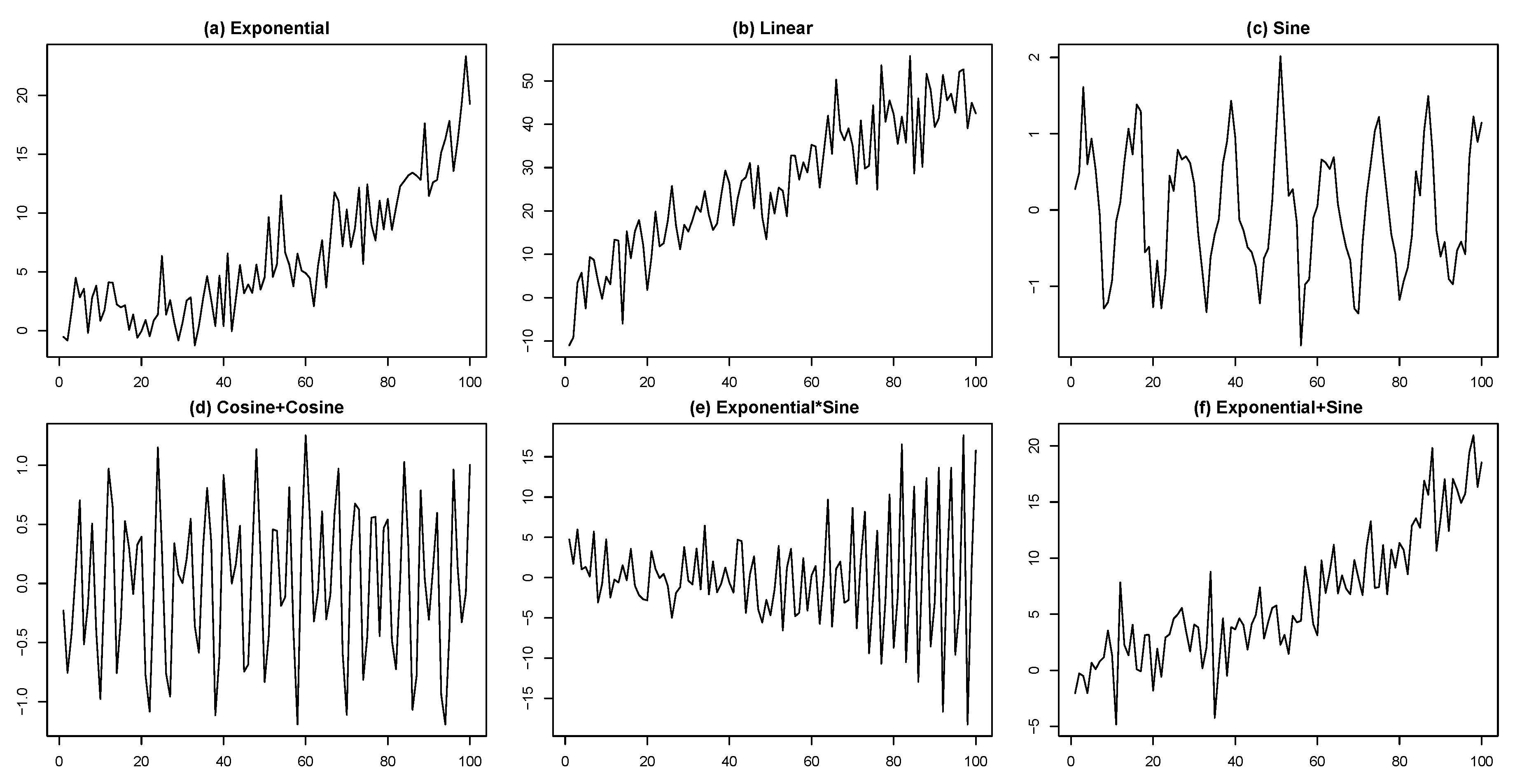
- (a)
- Exponential:.
- (b)
- Linear:.
- (c)
- Sine:.
- (d)
- Cosine+Cosine:.
- (e)
- Exponential×Sine:.
- (f)
- Exponential+Sine:.
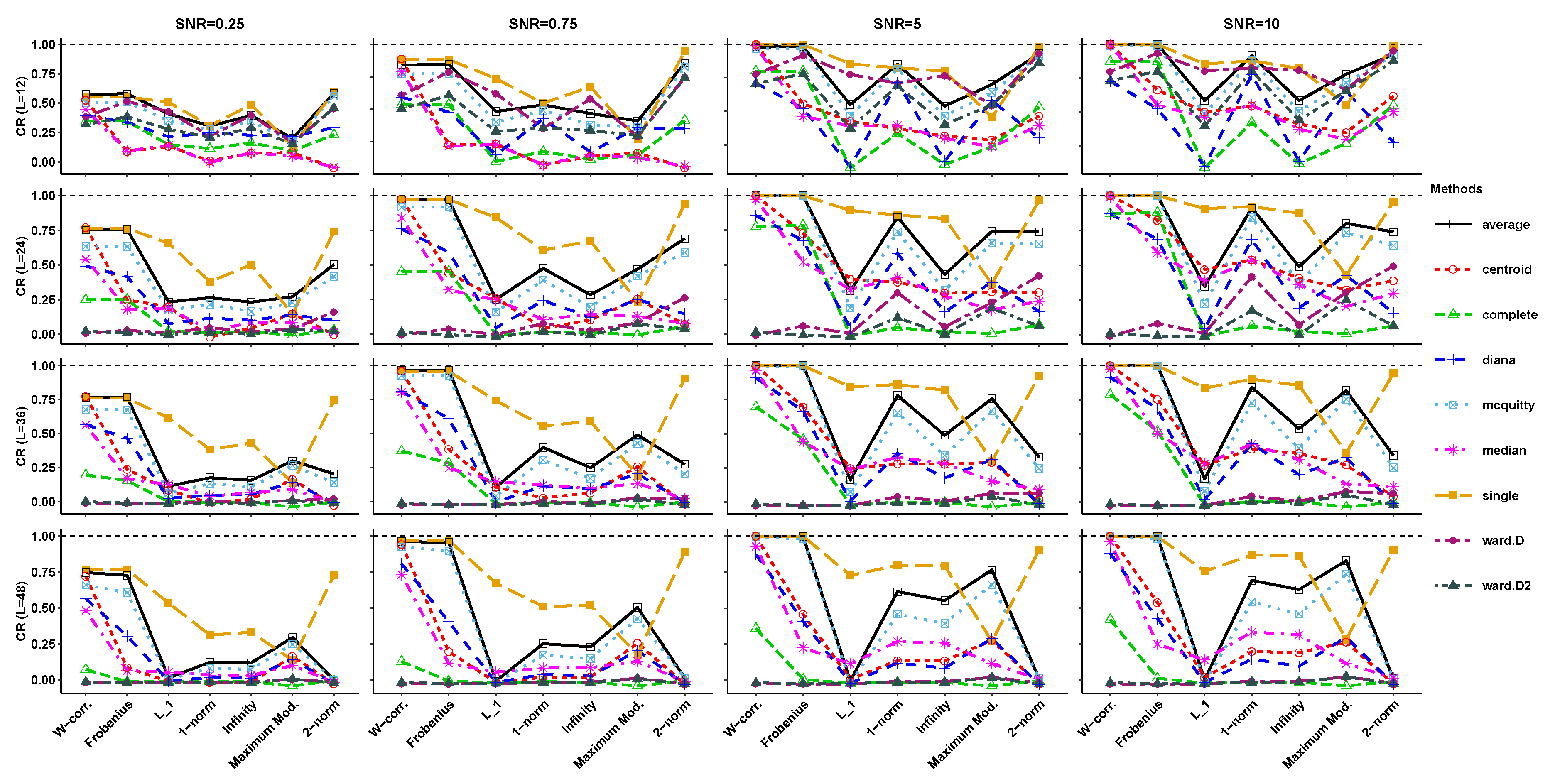
In this simulation, four signal to noise ratios (SNRs) including and 10 were used to assess the effect of the noise levels on the grouping results. The simulation was repeated 2000 times for each scenario (a–f) and for each SNR. In order to enable a better comparison based on the CR index, a dashed horizontal line is added to all figures of the CR index.
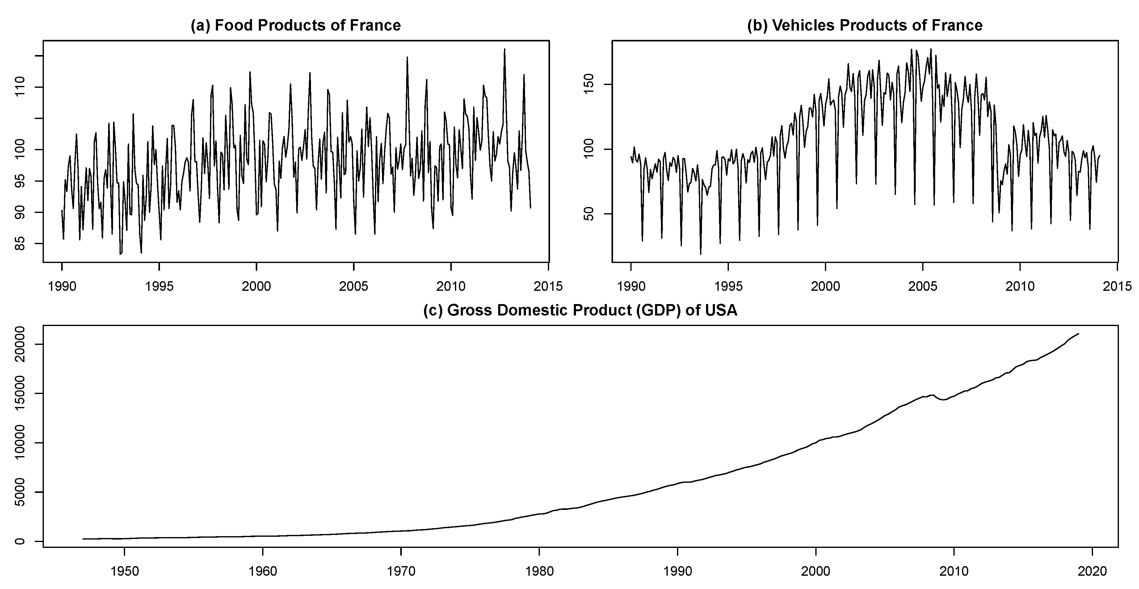
The simulated series (a–f) have various patterns including trend and periodicity. In order to observe the structure of each simulated series, the simulation was done once with . The time series plots are depicted in Figure 1.
Considering the theory of time series of finite rank proposed in [27], the simulated series (a–f) have finite rank. Therefore, it is possible to determine the “correct” groups. Table 1 shows the “correct” groups for each of the simulated series that are determined based on the rank of the corresponding trajectory matrices. For more details; see, [27].
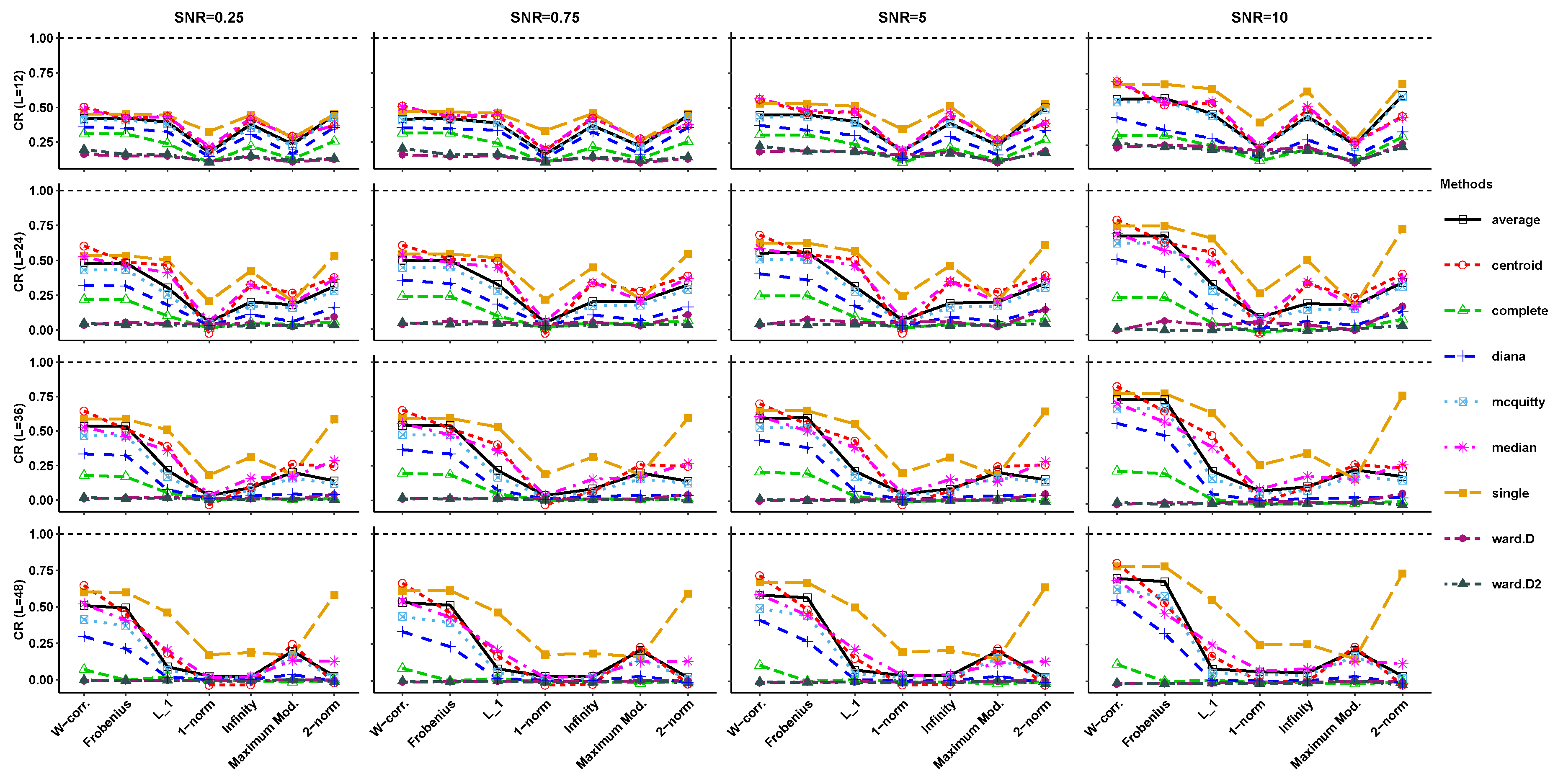
In Figure 2, the CR index is shown for the exponential series (case a) with different SNRs, which are computed for various hierarchical clustering algorithms and different values of the window length (L). It can be concluded that the ward.D and ward.D2 methods have the worst performance for each L, at each level of the SNR and for all clustering methods and all kinds of distances. However, clustering based on the w-correlation and the Frobenius norm results in the best performance, except for the complete method. In this case, the similarity between the grouping by the complete method and “correct” groups decrease as L increases. In addition, clustering based on , Infinity and 2-norm distances exhibit good performance in detecting the “correct” groups for . The capability of these distances goes to decline for a larger L except for the single method and 2-norm distance.
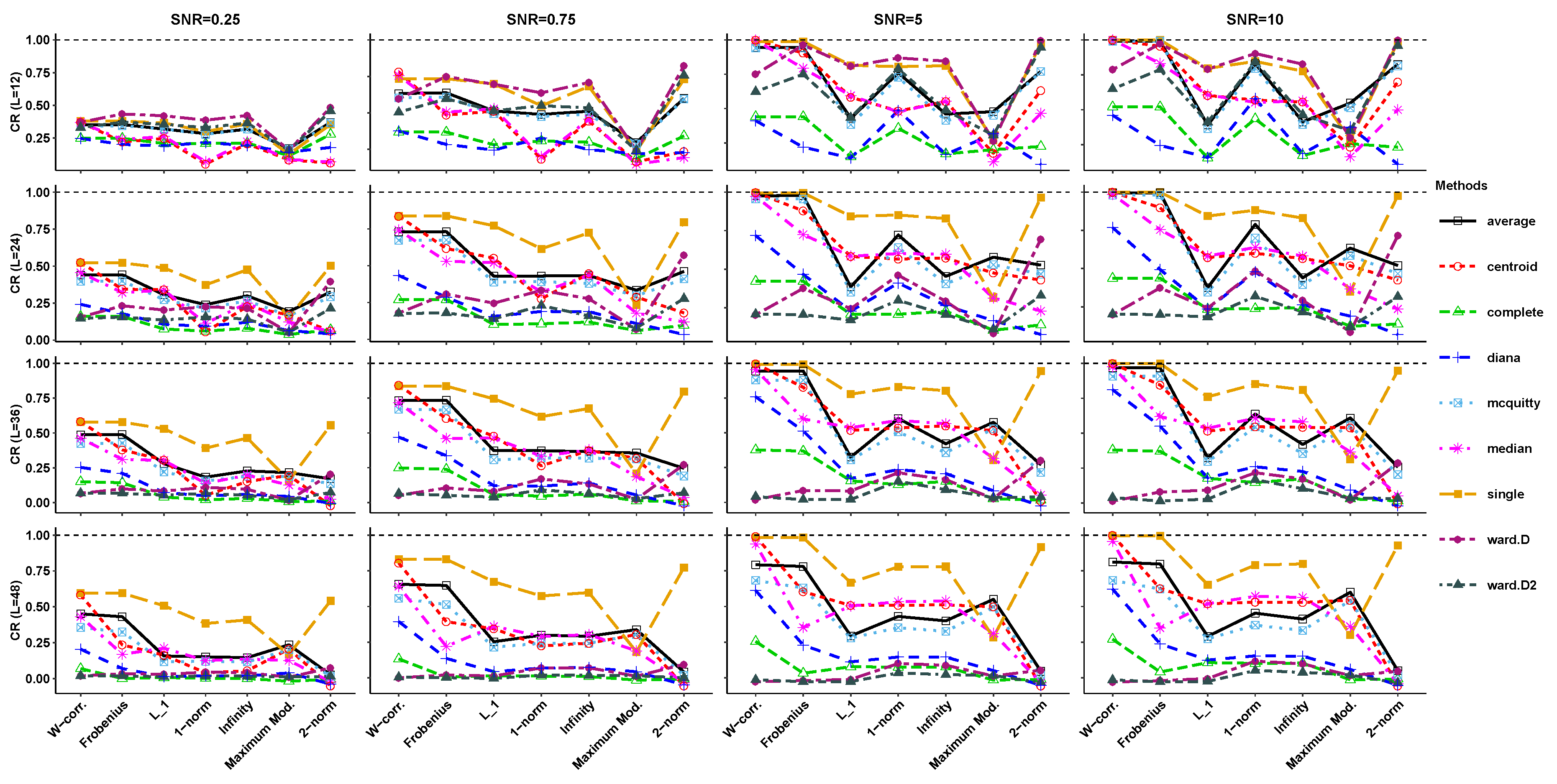
Figure 3 depicts the CR index for the linear series (case b). Similar to the case with an exponential series, the ward.D and ward.D2 methods can not provide a satisfactory result for each L, at each level of the SNR and all types of distances. Moreover, the efficiency of the clustering based on the w-correlation and the Frobenius norm is better than the other distances. In addition, the performance of , infinity and 2-norm distances are acceptable only for . The capability of these distances decreases for a larger L.
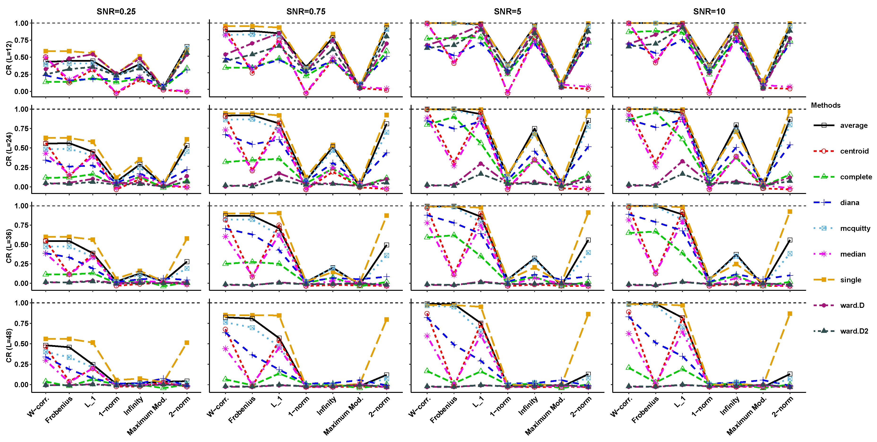
In Figure 4, the CR index for the Sine series (case c) is drawn. Similar to the simulated exponential and linear series, the output of ward.D and ward.D2 methods are not good for large L, at each level of the SNR and all types of distances. Additionally, the efficiency of the clustering based on the w-correlation and the Frobenius norm is better than the other distances. As can be seen in these figures, the single, average and McQuitty methods are better than other methods when the Frobenius norm is used to measure the dissimilarity. Another interesting find is that for large L and at each level of the SNR, the single method outperforms other methods if , 1-norm Infinity and 2-norm distances be used. However, the average and McQuitty methods are better than other methods for the maximum modulus norm.
Figure 5 presents the CR index for the cosine+cosine series (case d). Similar to the previous simulated series, at each level of the SNR and all types of distances, the utility of ward.D and ward.D2 methods goes to decline as L increases. Additionally, the superiority of the w-correlation and the Frobenius norms over the other distances are more visible for large SNR. As can be seen in these figures, for large L and at each level of the SNR, the single method outperforms other methods when the maximum modulus norm is not used. In the case with the maximum modulus norm, the average, McQuitty and centroid methods present better outputs.
Figure 6 depicts the CR index for the exponential×sine series (case e). This is similar to the previous simulated series; firstly, the efficiency of the clustering based on the w-correlation and the Frobenius norm is better than the other distances, especially for the single, average and McQuitty clustering methods. Secondly, the ward.D and ward.D2 methods can not provide a satisfactory result for large L, at each level of the SNR and all types of distances. It is noteworthy that in this simulated series, the norm shows a good performance, which is not obtained from the previous simulated series. It can be concluded from these figures that the single method is better than other methods for . In the case with and , the capability of the single method in detecting the "correct" groups is considerable when the 2-norm is used.
In Figure 7, the CR index for the exponential+sine series (case f) is drawn. The results that can be concluded from these figures are broadly similar to that of the exponential×sine series (case e); and thus, they are not repeated here.
5. Real-World Data
In this section, we compare the efficiency of hierarchical clustering methods along with different matrix norms using three real-world data. These real-world time series are as follows:
- Seasonally non-adjusted food and vehicle products of France from January 1990 to February 2014. These data are taken from INSEE (Institute National de la Statistique et des Etudes Economiques) including 290 observations. These series were previously used in [52,53,54]. Those interested in a summary of the data are referred to [52] instead of replicating this information here. The time series plots for these data, which are depicted in Figure 8, clearly show that they have a seasonal structure along with a non-linear trend.
- Gross domestic product (GDP) of the United States of America (USA) in billions of dollars from January 1947 to January 2019. This quarterly time series contains 289 observations that are taken from Federal Reserve Economic Data available at https://www.quandl.com/data/FRED/GDP. As shown in Figure 8, the GDP series is non-stationary with a non-linear trend that appears to increase exponentially over time.
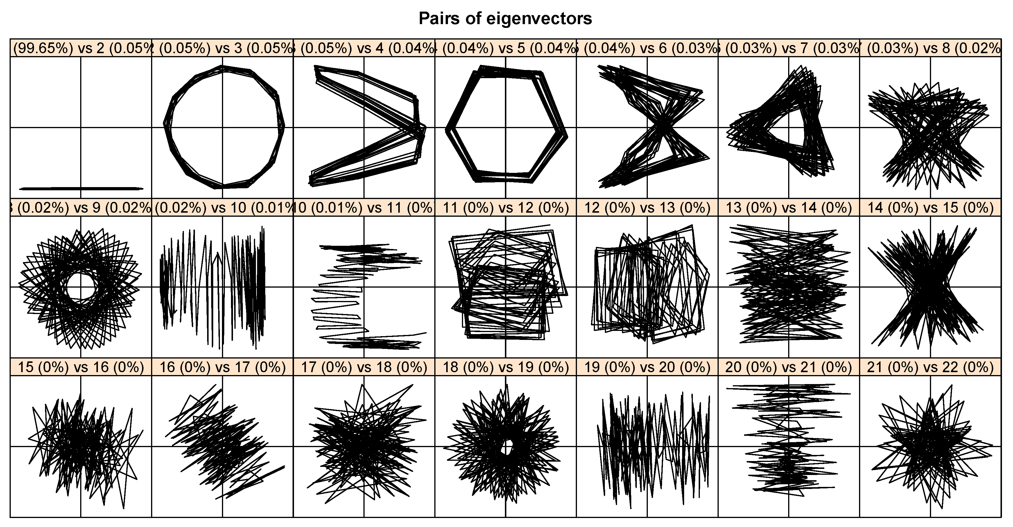
Table 2 reports the identified groups and window length (L) for the real-world time series. We chose the groups based on information obtained from one-dimensional figures of the eigenvectors , two-dimensional figures of the eigenvectors , and the matrix of the absolute values of the w-correlations. For example, consider the food product time series. The two-dimensional figures of the eigenvectors of this time series are shown in Figure 9. This figure, which is the scatter plot of successive eigenvectors, is used to detect the harmonic components with different frequencies. Each regular P-vertex polygon in the scatter plots of eigenvectors denotes a harmonic component with period P [27]. Therefore, for identifying the harmonic component it is sufficient to find regular P-vertex polygons, which may be in a spiral form. Corresponding pairs of eigenvectors identify the harmonic component. Hence, it can be concluded from Figure 9 that the pairs of eigenvectors 2–3, 4–5, 6–7, and 8–9 correspond to the harmonic components of food product time series. More details on the window length selection and group identification can be found in [1,29].
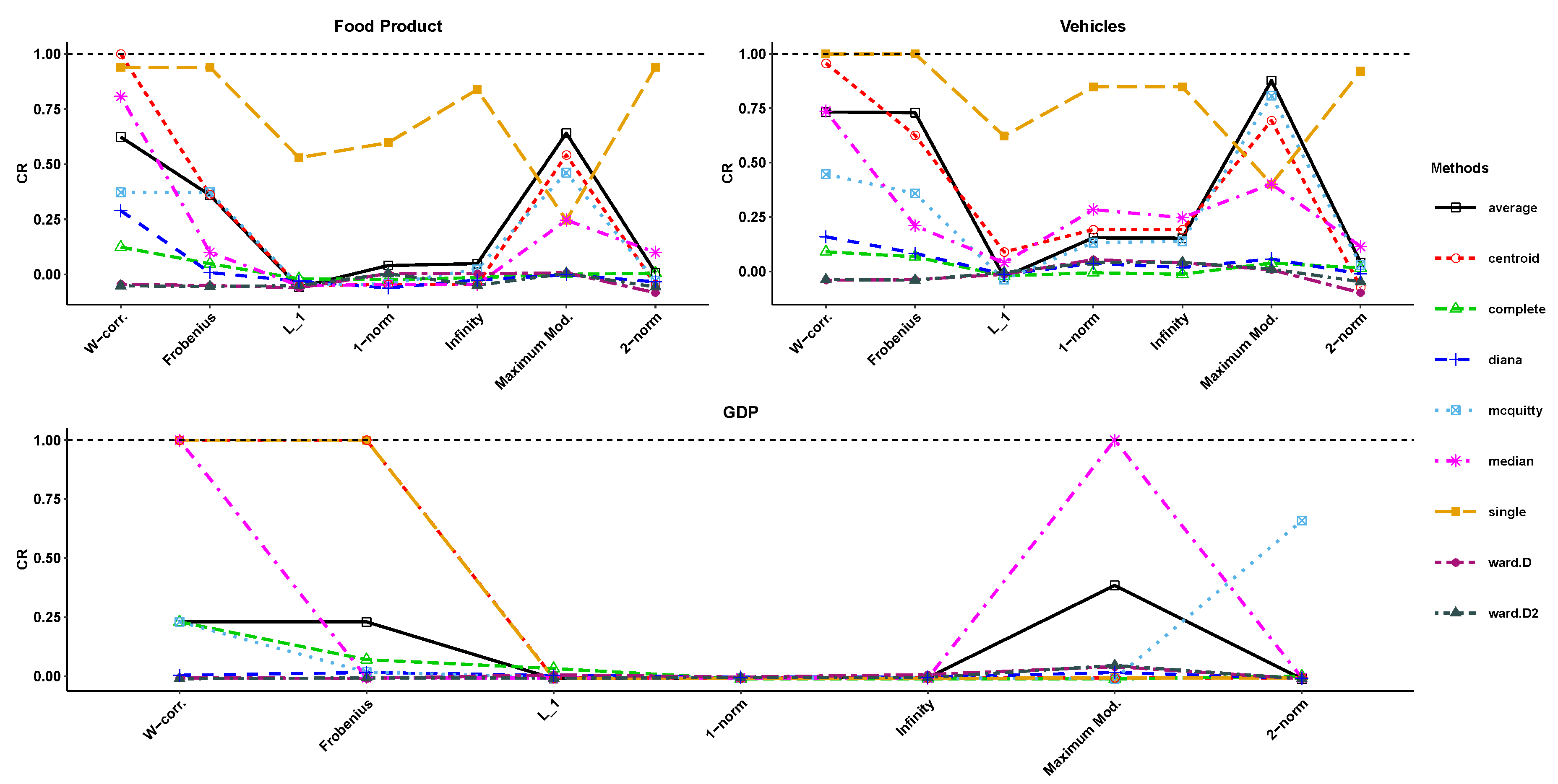
Figure 10 shows the CR index for the real-world time series. It can be concluded from this figure that, similar to the outputs of the simulation study, the ward.D and ward.D2 methods are unable to identify proper groups. In the food product series, centroid linkage with w-correlation-based distance is the best method. Additionally, the single method shows a good performance especially for w-correlation, Frobenius, and 2-norm. However, the average method is better than other methods for the maximum modulus norm.
In the vehicles series, the single linkage with w-correlation and Frobenius norms are the best methods. Note that the centroid linkage performs well only for w-correlation-based distance. Similar to the food product series, the average method is better than other methods for the maximum modulus norm, which is in accordance with the simulation results for harmonic series (cases c and d).
In the GDP series, hierarchical clustering with the single and centroid linkages can exactly split the components into the groups reported in Table 2. This result is also true for the median linkage with the w-correlation and maximum modulus norm.
6. Conclusions
In this paper, we have proposed a novel dissimilarity measure between components of a time series based on various matrix norms such as Frobenius, -norm, 1-norm, 2-norm and so on. Various matrix norms result in different distance matrices that can be used to cluster eigentriples at the grouping step of SSA by means of distance-based clustering methods such as hierarchical clustering techniques. In this research, a comparison study has been conducted in order to find a suitable matrix norm and a proper hierarchical clustering method to identify appropriate groups in SSA. In general, the simulation results and real-world data applications indicated that the accuracy of clustering based on the w-correlation and the Frobenius norm is better than other distance measures. Also, the results support the idea that single linkage along with 2-norm can provide satisfactory automatic grouping. However, the evidence from this study implies that the ward.D and ward.D2 linkages could not detect meaningful groups.
Despite these explicit findings, determining the best hierarchical clustering linkage is not a straightforward procedure. It depends on the structure of the time series and the level of SNR. For example, in the exponential synthetic data (case a) and the GDP series, which includes an exponential-like trend, the efficiency of the single, centroid and median linkages are almost similar, and these techniques outperform the other method. Additionally, in a time series with a seasonal pattern, it seems that the single and average linkages are able to separate periodic components from noise. In summary, findings of this investigation suggest that automatic grouping of eigentriples using the single, average, centroid, and median linkages by means of the w-correlation and the Frobenius norm as distance measures, can lead to more accurate results.
Author Contributions
Conceptualization, H.H., M.K. and H.H., M.K.; Methodology, H.H., M.K.; Investigation, H.H., M.K.; Writing—review and editing, H.H., M.K.
Funding
This research received no external funding.
Conflicts of Interest
The authors declare no conflict of interest.
References
- Golyandina, N.; Zhigljavsky, A. Singular Spectrum Analysis for Time Series; Springer Briefs in Statistics; Springer: New York, NY, USA, 2013. [Google Scholar]
- Aydin, S.; Saraoglu, H.M.; Kara, S. Singular Spectrum Analysis of Sleep EEG in Insomnia. J. Med. Syst. 2011, 35, 457–461. [Google Scholar] [CrossRef]
- Sanei, S.; Hassani, H. Singular Spectrum Analysis of Biomedical Signals; Taylor & Francis/CRC: Boca Raton, FL, USA, 2016. [Google Scholar]
- Hassani, H.; Yeganegi, M.R.; Silva, E.S. A New Signal Processing Approach for Discrimination of EEG Recordings. Stats 2018, 1, 155–168. [Google Scholar] [CrossRef] [Green Version]
- Safi, S.M.M.; Pooyan, M.; Nasrabadi, A.M. Improving the performance of the SSVEP-based BCI system using optimized singular spectrum analysis (OSSA). Biomed. Signal Proces. Control 2018, 46, 46–58. [Google Scholar] [CrossRef]
- Ghodsi, Z.; Silva, E.S.; Hassani, H. Bicoid Signal Extraction with a Selection of Parametric and Nonparametric Signal Processing Techniques. Genom. Proteom. Bioinform. 2015, 13, 183–191. [Google Scholar] [CrossRef] [PubMed] [Green Version]
- Movahedifar, M.; Yarmohammadi, M.; Hassani, H. Bicoid signal extraction: Another powerful approach. Math. Biosci. 2018, 303, 52–61. [Google Scholar] [CrossRef] [PubMed]
- Carvalho, M.; Rodrigues, P.C.; Rua, A. Tracking the US business cycle with a singular spectrum analysis. Econ. Lett. 2012, 114, 32–35. [Google Scholar] [CrossRef]
- Hassani, H.; Silva, E.S.; Gupta, R.; Segnon, M.K. Forecasting the price of gold. Appl. Econ. 2015, 47, 4141–4152. [Google Scholar] [CrossRef]
- Silva, E.S.; Ghodsi, Z.; Ghodsi, M.; Heravi, S.; Hassani, H. Cross country relations in European tourist arrivals. Ann. Tour. Res. 2017, 63, 151–168. [Google Scholar] [CrossRef]
- Arteche, J.; Garcia-Enriquez, J. Singular Spectrum Analysis for signal extraction in Stochastic Volatility models. Econom. Stat. 2017, 1, 85–98. [Google Scholar] [CrossRef]
- Groth, A.; Ghil, M. Synchronization of world economic activity. Chaos Interdiscip. J. Nonlinear Sci. 2017, 27, 127002. [Google Scholar] [CrossRef] [Green Version]
- Groth, A.; Ghil, M. Multivariate singular spectrum analysis and the road to phase synchronization. Phys. Rev. E 2011, 84, 036206. [Google Scholar] [CrossRef] [PubMed] [Green Version]
- Mahmoudvand, R.; Rodrigues, P.C. Predicting the Brexit Outcome Using Singular Spectrum Analysis. J. Comput. Stat. Model. 2018, 1, 9–15. [Google Scholar]
- Saayman, A.; Klerk, J. Forecasting tourist arrivals using multivariate singular spectrum analysis. Tour. Econ. 2019, 25, 330–354. [Google Scholar] [CrossRef]
- Hassani, H.; Rua, A.; Silva, E.S.; Thomakos, D. Monthly forecasting of GDP with mixed-frequency multivariate singular spectrum analysis. Int. J. Forecast. 2019, 35, 1263–1272. [Google Scholar] [CrossRef] [Green Version]
- Rocco S, C.M. Singular spectrum analysis and forecasting of failure time series. Reliab. Eng. Syst. Saf. 2013, 114, 126–136. [Google Scholar] [CrossRef]
- Muruganatham, B.; Sanjith, M.A.; Krishnakumar, B.; Satya Murty, S.A.V. Roller element bearing fault diagnosis using singular spectrum analysis. Mech. Syst. Signal Process. 2013, 35, 150–166. [Google Scholar] [CrossRef]
- Chen, Q.; Dam, T.V.; Sneeuw, N.; Collilieux, X.; Weigelt, M.; Rebischung, P. Singular spectrum analysis for modeling seasonal signals from GPS time series. J. Geodyn. 2013, 72, 25–35. [Google Scholar] [CrossRef]
- Hou, Z.; Wen, G.; Tang, P.; Cheng, G. Periodicity of Carbon Element Distribution Along Casting Direction in Continuous-Casting Billet by Using Singular Spectrum Analysis. Metall. Mater. Trans. B 2014, 45, 1817–1826. [Google Scholar] [CrossRef]
- Liu, K.; Law, S.S.; Xia, Y.; Zhu, X.Q. Singular spectrum analysis for enhancing the sensitivity in structural damage detection. J. Sound Vib. 2014, 333, 392–417. [Google Scholar] [CrossRef]
- Bail, K.L.; Gipson, J.M.; MacMillan, D.S. Quantifying the Correlation Between the MEI and LOD Variations by Decomposing LOD with Singular Spectrum Analysis. In Earth on the Edge: Science for a Sustainable Planet International Association of Geodesy Symposia; Springer: Berlin/Heidelberg, Germany, 2014; Volume 139, pp. 473–477. [Google Scholar]
- Chao, H.-S.; Loh, C.-H. Application of singular spectrum analysis to structural monitoring and damage diagnosis of bridges. Struct. Infrastruct. Eng. Maint. Manag. Life-Cycle Des. Perform. 2014, 10, 708–727. [Google Scholar] [CrossRef]
- Khan, M.A.R.; Poskitt, D.S. Forecasting stochastic processes using singular spectrum analysis: Aspects of the theory and application. Int. J. Forecast. 2017, 33, 199–213. [Google Scholar] [CrossRef]
- Lahmiri, S. Minute-ahead stock price forecasting based on singular spectrum analysis and support vector regression. Appl. Math. Comput. 2018, 320, 444–451. [Google Scholar] [CrossRef]
- Poskitt, D.S. On Singular Spectrum Analysis and Stepwise Time Series Reconstruction. J. Time Ser. Anal. 2019. [Google Scholar] [CrossRef]
- Golyandina, N.; Nekrutkin, V.; Zhigljavsky, A. Analysis of Time Series Structure: SSA and Related Techniques; Chapman & Hall/CRC: London, UK, 2001. [Google Scholar]
- Hassani, H.; Mahmoudvand, R. Singular Spectrum Analysis Using R; Palgrave Macmillan: Basingstoke, UK, 2018. [Google Scholar]
- Golyandina, N.; Korobeynikov, A.; Zhigljavsky, A. Singular Spectrum Analysis with R; Springer: Berlin/Heidelberg, Germany, 2018. [Google Scholar]
- Golyandina, N. Particularities and commonalities of singular spectrum analysis as a method of time series analysis and signal processing. arXiv 2019, arXiv:1907.02579v1. [Google Scholar]
- Alexandrov, T.; Golyandina, N. Automatic extraction and forecast of time series cyclic components within the framework of SSA. In Proceedings of the 5th St.Petersburg Workshop on Simulation, Saint Petersburg, Russia, 26 June–2 July 2005; pp. 45–50. Available online: http://www.gistatgroup.com/gus/autossa2.pdf (accessed on 2 October 2019).
- Bilancia, M.; Campobasso, F. Airborne particulate matter and adverse health events: Robust estimation of timescale effects. In Classification as a Tool for Research; Locarek-Junge, H., Weihs, C., Eds.; Springer: Berlin/Heidelberg, Germany, 2010; pp. 481–489. [Google Scholar]
- Hassani, H. Singular Spectrum Analysis: Methodology and Comparison. J. Data Sci. 2007, 5, 239–257. [Google Scholar]
- Broomhead, D.; King, G. Extracting qualitative dynamics from experimental data. Physica D 1986, 20, 217–236. [Google Scholar] [CrossRef]
- Broomhead, D.; King, G. On the qualitative analysis of experimental dynamical systems. In Nonlinear Phenomena and Chaos; Sarkar, S., Ed.; Adam Hilger: Bristol, UK, 1986; pp. 113–144. [Google Scholar]
- Proschan, M.A.; Shaw, P.A. Essential of Probability Theory for Statisticians; Chapman & Hall/CRC: London, UK, 2016. [Google Scholar]
- Golub, G.H.; Loan, C.F.V. Matrix Computations, 4th ed.; The John Hopkins University Press: Baltimore, UK, 2013. [Google Scholar]
- Korobeynikov, A. Computation- and space-efficient implementation of SSA. Stat. Its Interface 2010, 3, 257–368. [Google Scholar] [CrossRef]
- Golyandina, N.; Korobeynikov, A. Basic Singular Spectrum Analysis and forecasting with R. Comput. Stat. Data Anal. 2014, 71, 934–954. [Google Scholar] [CrossRef]
- Golyandina, N.; Korobeynikov, A.; Shlemov, A.; Usevich, K. Multivariate and 2D Extensions of Singular Spectrum Analysis with the Rssa Package. J. Stat. Softw. 2015, 67, 1–78. [Google Scholar] [CrossRef]
- Kaufman, L.; Rousseeuw, P.J. Finding Groups in Data: An Introduction to Cluster Analysis; Wiley: New York, NY, USA, 1990. [Google Scholar]
- Johnson, R.A.; Wichern, D.W. Applied Multivariate Statistical Analysis, 6th ed.; Pearson Education Limited: Harlow, UK, 2013. [Google Scholar]
- Maechler, M.; Rousseeuw, P.; Struyf, A.; Hubert, M.; Hornik, K. Cluster: Cluster Analysis Basics and Extensions; R Package Version 2.0.7-1; R Package Vignette: Madison, WI, USA, 2018. [Google Scholar]
- R Core Team. R: A Language and Environment for Statistical Computing; R Foundation for Statistical Computing: Vienna, Austria, 2018; Available online: https://www.R-project.org/ (accessed on 2 October 2019).
- Charrad, M.; Ghazzali, N.; Boiteau, V.; Niknafs, A. NbClust: An R Package for Determining the Relevant Number of Clusters in a Data Set. J. Stat. Softw. 2014, 61, 1–36. [Google Scholar] [CrossRef]
- Contreras, P.; Murtagh, F. Hierarchical Clustering. In Handbook of Cluster Analysis; Henning, C., Meila, M., Murtagh, F., Rocci, R., Eds.; Chapman & Hall/CRC: London, UK, 2016; pp. 103–123. [Google Scholar]
- Gordon, A.D. Classification, 2nd ed.; Chapman and Hall: London, UK, 1999. [Google Scholar]
- Hubert, L.; Arabie, P. Comparing partitions. J. Classif. 1985, 2, 193–218. [Google Scholar] [CrossRef]
- Gates, A.J.; Ahn, Y.Y. The impact of random models on clustering similarity. J. Mach. Learn. Res. 2017, 18, 1–28. [Google Scholar]
- Vinh, N.X.; Epps, J.; Bailey, J. Information theoretic measures for clusterings comparison: Variants, properties, normalization and correction for chance. J. Mach. Learn. Res. 2010, 11, 2837–2854. [Google Scholar]
- Hennig, C. fpc: Flexible Procedures for Clustering, R package version 2.1-11.1; R Package Vignette: Madison, WI, USA, 2018; Available online: https://CRAN.R-project.org/package=fpc (accessed on 2 October 2019).
- Silva, E.S.; Hassani, H.; Heravi, S. Modeling European industrial production with multivariate singular spectrum analysis: A cross-industry analysis. J. Forecast. 2018, 37, 371–384. [Google Scholar] [CrossRef]
- Hassani, H.; Heravi, H.; Zhigljavsky, A. Forecasting European industrial production with singular spectrum analysis. Int. J. Forecast. 2009, 25, 103–118. [Google Scholar] [CrossRef]
- Heravi, S.; Osborn, D.R.; Birchenhall, C.R. Linear versus neural network forecasts for European industrial production series. Int. J. Forecast. 2004, 20, 435–446. [Google Scholar] [CrossRef]
Figure 1.
Time series plots of simulated series.

Figure 2.
Corrected Rand (CR) index for the exponential series (case a).

Figure 3.
CR index for the linear series (case b).

Figure 4.
CR index for the sine series (case c).

Figure 5.
CR index for the cosine+cosine series (case d).

Figure 6.
CR index for the Exponential×sine series (case e).

Figure 7.
CR index for the exponential+sine series (case f).

Figure 8.
Time series plot of real-world data.

Figure 9.
Scatter plots of eigenvectors for food products time series.

Figure 10.
The CR index for the real-world time series.


Table 1.
Correct groups of the simulated series.
| Simulated Series | Correct Groups |
|---|---|
| Exponential | |
| Linear | |
| Sine | |
| Cosine+Cosine | |
| Exponential×Sine | |
| Exponential+Sine |
Table 2.
Identified groups of the real time series.
| Real Time Series | L | Groups |
|---|---|---|
| Food product | 144 | |
| Vehicles | 144 | |
| GDP | 144 |
© 2019 by the authors. Licensee MDPI, Basel, Switzerland. This article is an open access article distributed under the terms and conditions of the Creative Commons Attribution (CC BY) license (http://creativecommons.org/licenses/by/4.0/).
Share and Cite
MDPI and ACS Style
Kalantari, M.; Hassani, H. Automatic Grouping in Singular Spectrum Analysis. Forecasting 2019, 1, 189-204. https://0-doi-org.brum.beds.ac.uk/10.3390/forecast1010013
AMA Style
Kalantari M, Hassani H. Automatic Grouping in Singular Spectrum Analysis. Forecasting. 2019; 1(1):189-204. https://0-doi-org.brum.beds.ac.uk/10.3390/forecast1010013
Chicago/Turabian StyleKalantari, Mahdi, and Hossein Hassani. 2019. "Automatic Grouping in Singular Spectrum Analysis" Forecasting 1, no. 1: 189-204. https://0-doi-org.brum.beds.ac.uk/10.3390/forecast1010013