Machine Learning-Based Error Modeling to Improve GPM IMERG Precipitation Product over the Brahmaputra River Basin

 , ,
, , 
Abstract
:1. Introduction
2. Study Area and Datasets
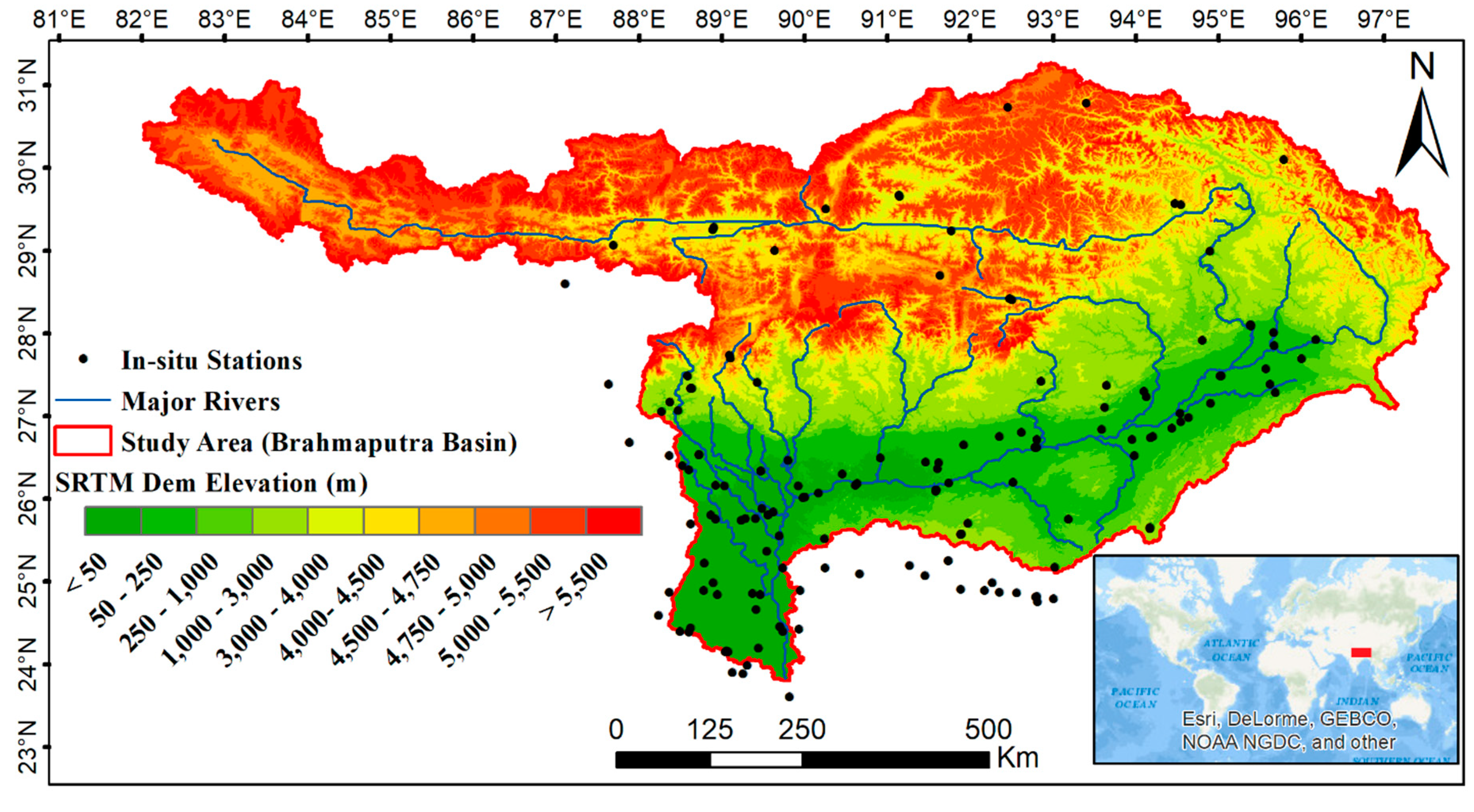
2.1. Study Area
2.2. Datasets
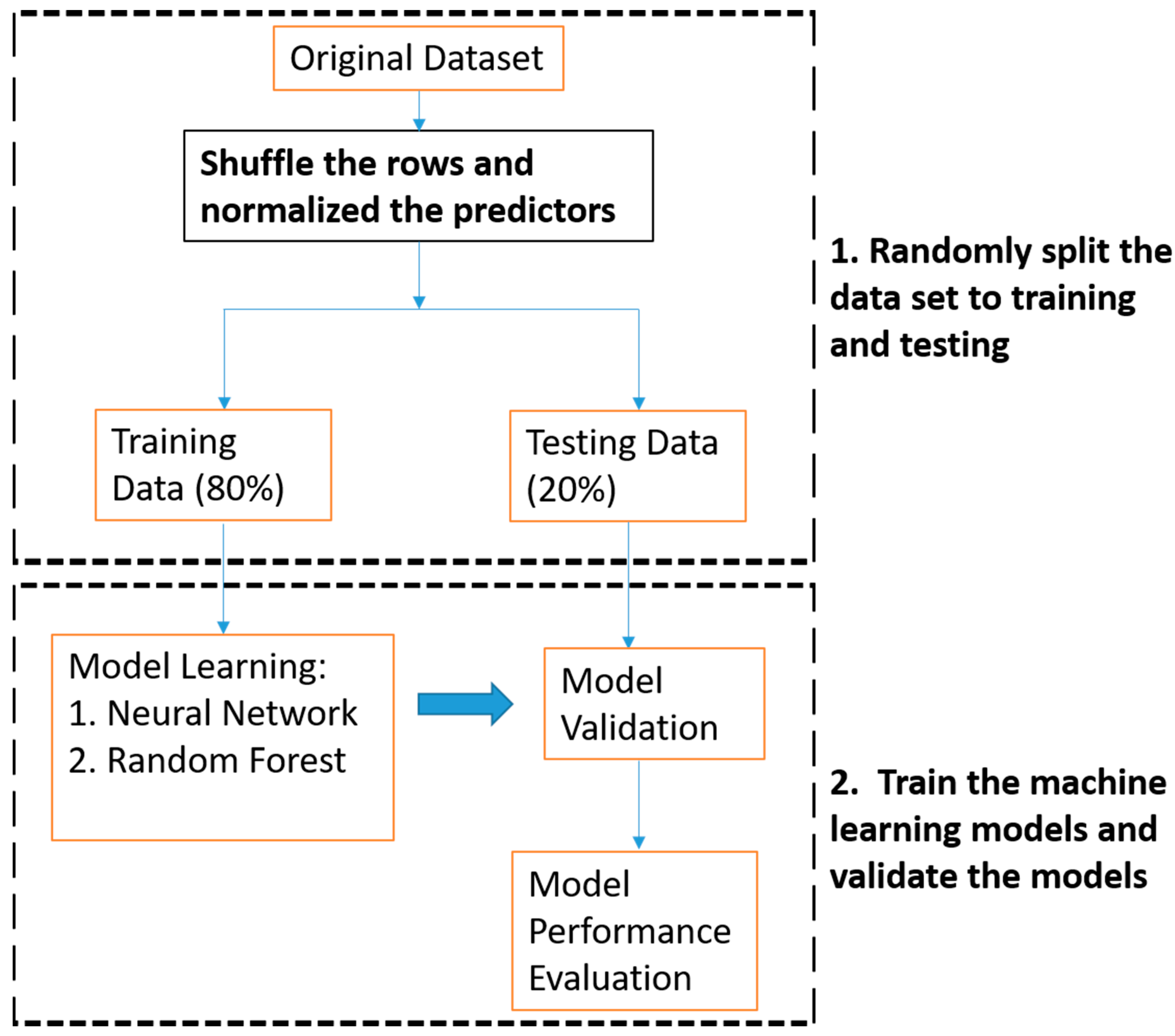
3. Methodology
3.1. Precipitation Error Modeling
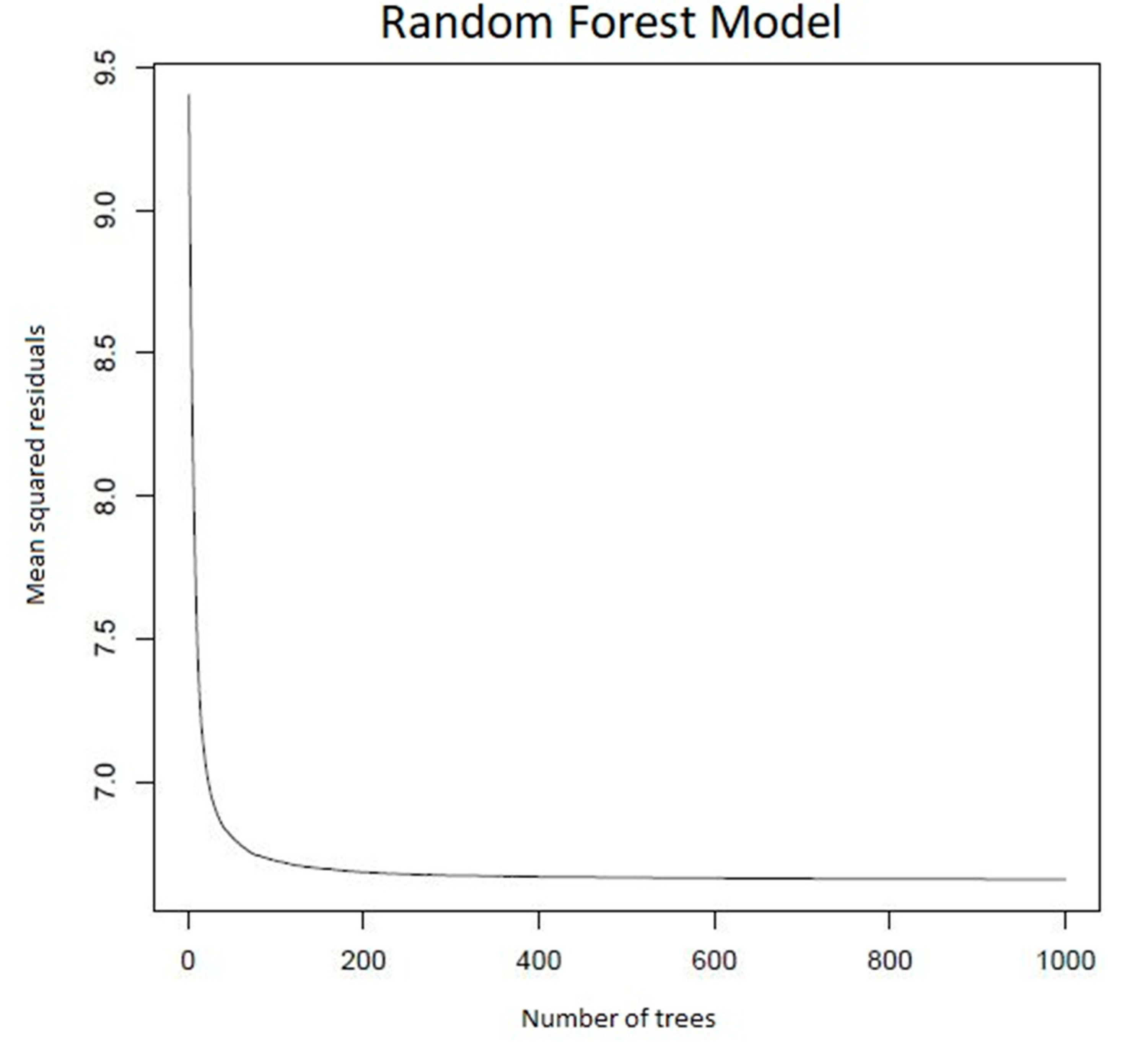
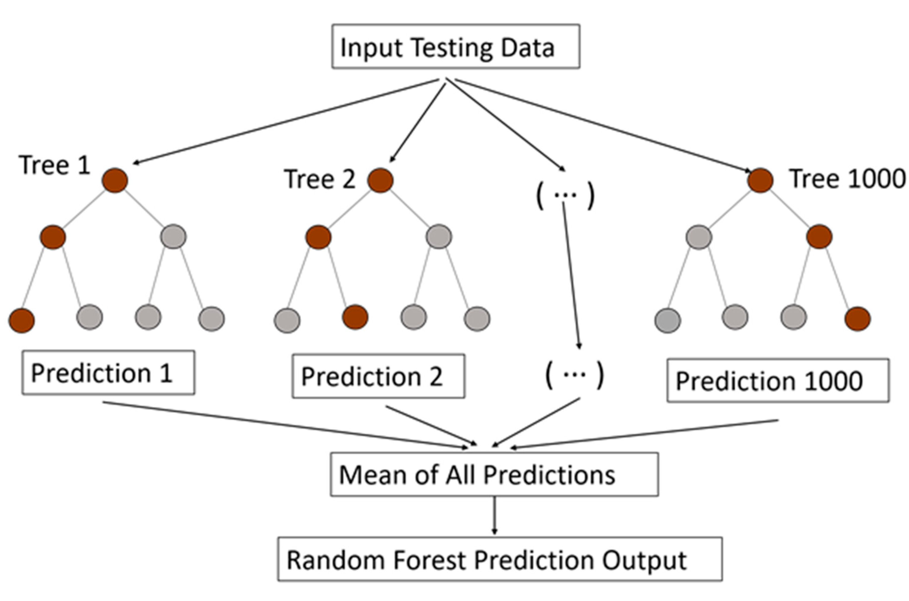
3.1.1. Random Forests (RF)
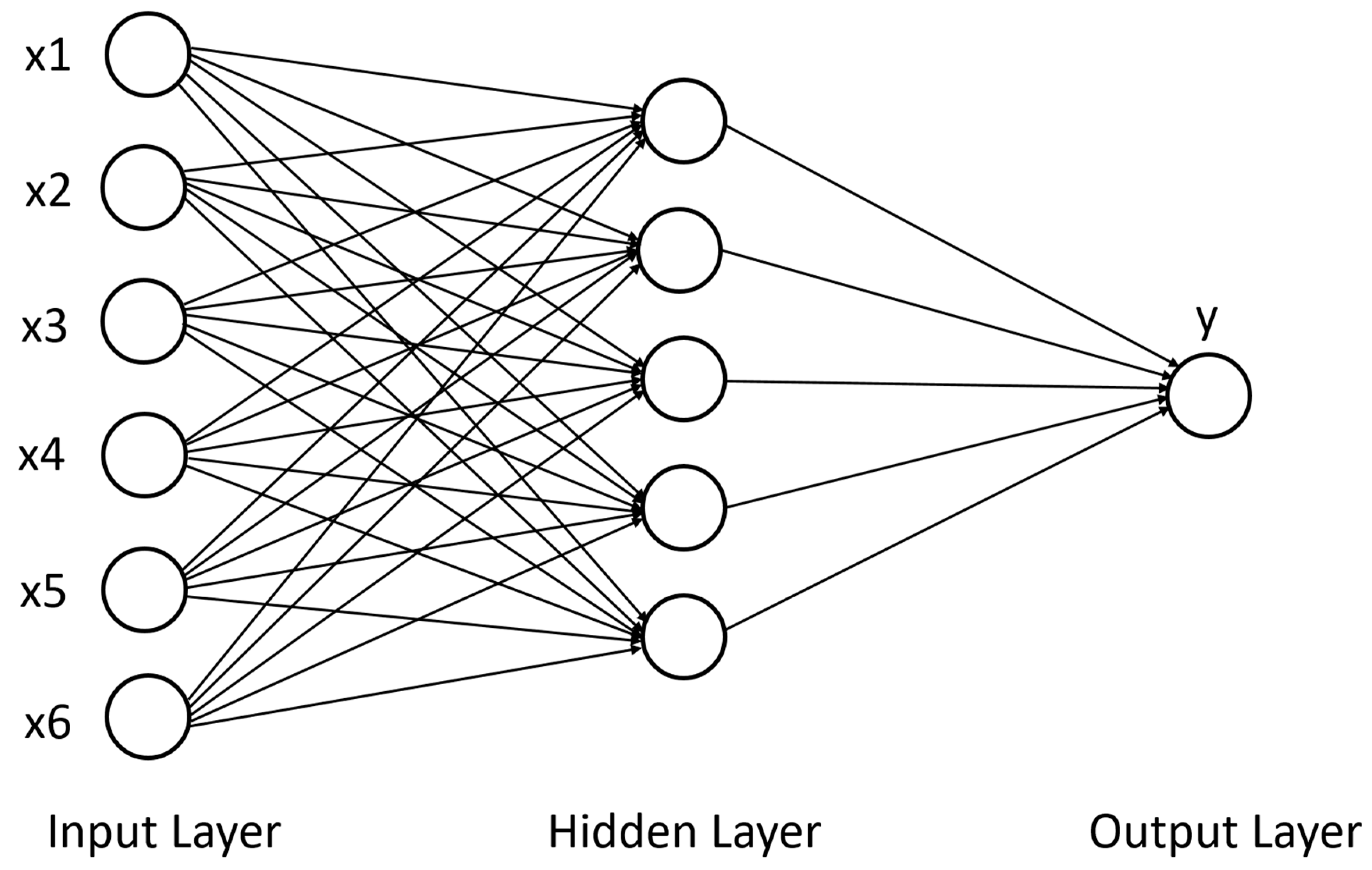
3.1.2. Neural Network (NN)
3.2. Performance Evaluation Error Metrics
4. Results
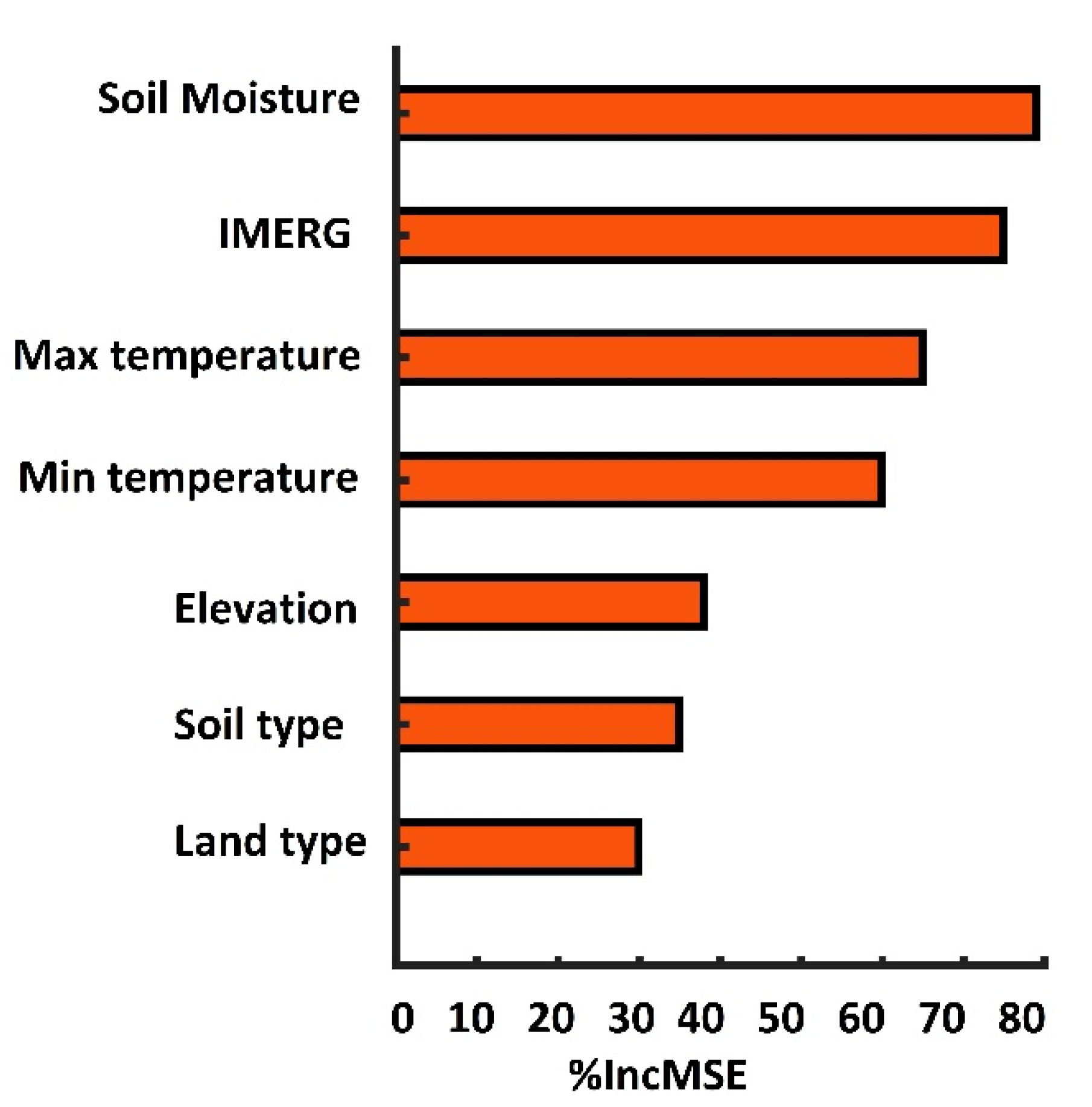
4.1. Variable Importance
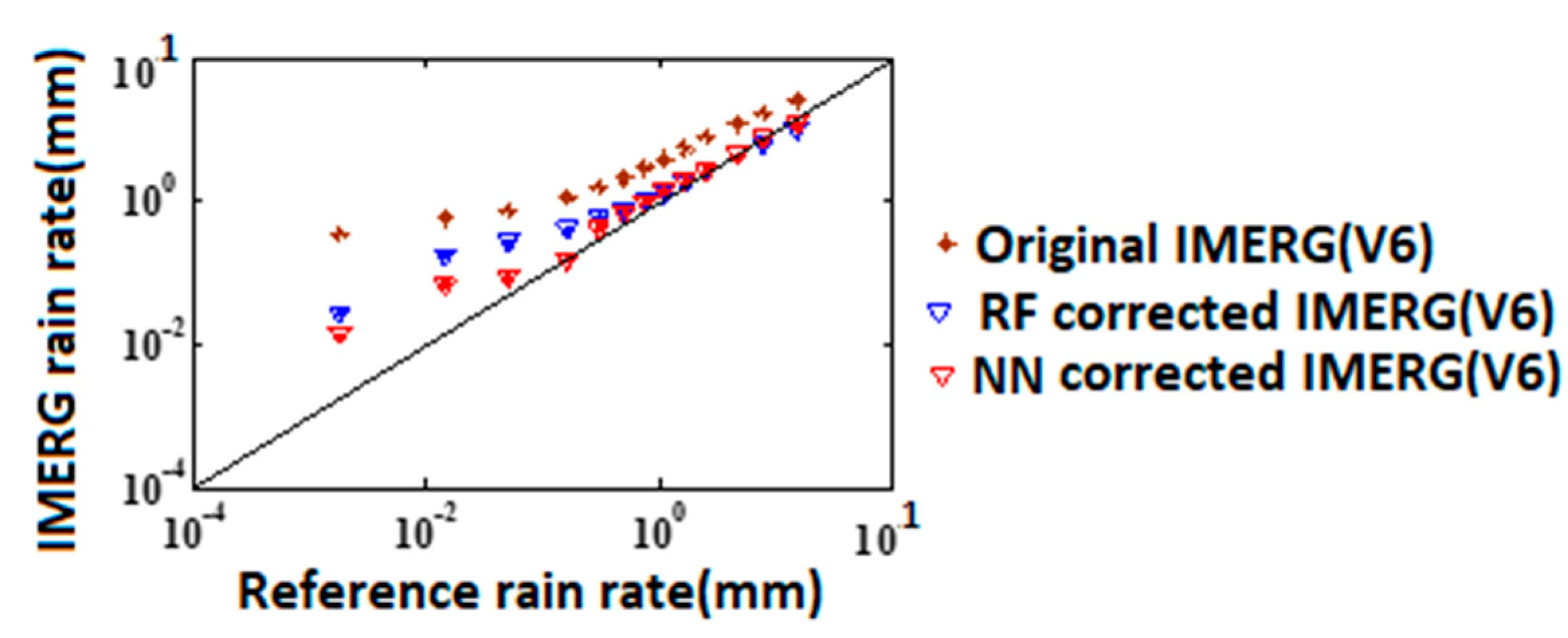
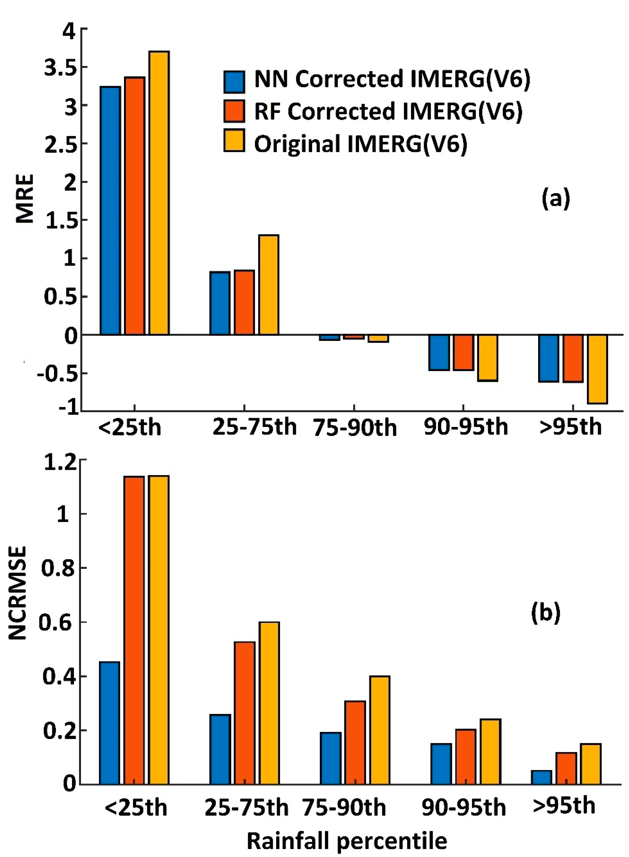
4.2. Evaluation of Error Model Corrected Rainfall Rates
4.3. Discussion
5. Conclusions
Author Contributions
Funding
Acknowledgments
Conflicts of Interest
References
- Liu, Z. Comparison of versions 6 and 7 3-hourly TRMM multi-satellite precipitation analysis (TMPA) research products. Atmos. Res. 2015, 163, 91–101. [Google Scholar] [CrossRef] [Green Version]
- Sun, Q.; Miao, C.; Duan, Q.; Ashouri, H.; Sorooshian, S.; Hsu, K. A Review of Global Precipitation Data Sets: Data Sources, Estimation, and Intercomparisons. Rev. Geophys. 2018, 56, 79–107. [Google Scholar] [CrossRef] [Green Version]
- Liu, Z. Comparison of Integrated Multisatellite Retrievals for GPM (IMERG) and TRMM Multisatellite Precipitation Analysis (TMPA) Monthly Precipitation Products: Initial Results. J. Hydrometeorol. 2016, 17, 777–790. [Google Scholar] [CrossRef]
- Steinschneider, S.; Ray, P.; Rahat, S.H.; Kucharski, J. A Weather-Regime-Based Stochastic Weather Generator for Climate Vulnerability Assessments of Water Systems in the Western United States. Water Resour. Res. 2019, 55, 6923–6945. [Google Scholar] [CrossRef]
- Trenberth, K. Changes in precipitation with climate change. Clim. Res. 2011, 47, 123–138. [Google Scholar] [CrossRef] [Green Version]
- Huffman, G.J.; Bolvin, D.T.; Braithwaite, D.; Hsu, K.; Joyce, R.; Kidd, C.; Nelkin, E.J.; Xie, P. NASA Global Precipitation Measurement Integrated Multi-satellitE Retrievals for GPM (IMERG). Algorithm Theor. Basis Doc. 2015, 6, 30. [Google Scholar]
- Hou, A.Y.; Kakar, R.K.; Neeck, S.; Azarbarzin, A.A.; Kummerow, C.D.; Kojima, M.; Oki, R.; Nakamura, K.; Iguchi, T. The Global Precipitation Measurement Mission. Bull. Am. Meteorol. Soc. 2014, 95, 701–722. [Google Scholar] [CrossRef]
- Grecu, M.; Olson, W.S.; Munchak, S.J.; Ringerud, S.; Liao, L.; Haddad, Z.; Kelley, B.L.; McLaughlin, S.F. The GPM Combined Algorithm. J. Atmos. Ocean. Technol. 2016, 33, 2225–2245. [Google Scholar] [CrossRef]
- Smith, E.A.; Asrar, G.; Furuhama, Y.; Ginati, A.; Mugnai, A.; Nakamura, K.; Adler, R.F.; Chou, M.-D.; Desbois, M.; Durning, J.F.; et al. International Global Precipitation Measurement (GPM) Program and Mission: An Overview. In Measuring Precipitation from Space; Springer: Dordrecht, The Netherlands, 2007; pp. 611–653. [Google Scholar]
- Derin, Y.; Anagnostou, E.; Berne, A.; Borga, M.; Boudevillain, B.; Buytaert, W.; Chang, C.-H.; Delrieu, G.; Hong, Y.; Hsu, Y.C.; et al. Multiregional Satellite Precipitation Products Evaluation over Complex Terrain. J. Hydrometeorol. 2016, 17, 1817–1836. [Google Scholar] [CrossRef]
- Mei, Y.; Anagnostou, E.N.; Nikolopoulos, E.I.; Borga, M. Error Analysis of Satellite Precipitation Products in Mountainous Basins. J. Hydrometeorol. 2014, 15, 1778–1793. [Google Scholar] [CrossRef]
- Houze, R.A., Jr. Orographic effects on precipitating clouds. Rev. Geophys. 2012, 50, 289. [Google Scholar] [CrossRef]
- Roe, G.H. Orographic Precipitation. Annu. Rev. Earth Planet. Sci. 2005, 33, 645–671. [Google Scholar] [CrossRef]
- Bhuiyan, M.A.E.; Nikolopoulos, E.I.; Anagnostou, E.N.; Quintana-Seguí, P.; Barella-Ortiz, A. A nonparametric statistical technique for combining global precipitation datasets: Development and hydrological evaluation over the Iberian Peninsula. Hydrol. Earth Syst. Sci. 2018, 22, 1371–1389. [Google Scholar] [CrossRef] [Green Version]
- Ehsan Bhuiyan, M.A.; Nikolopoulos, E.I.; Anagnostou, E.N. Machine Learning–Based Blending of Satellite and Reanalysis Precipitation Datasets: A Multiregional Tropical Complex Terrain Evaluation. J. Hydrometeorol. 2019, 20, 2147–2161. [Google Scholar] [CrossRef]
- Ehsan Bhuiyan, M.A.; Nikolopoulos, E.I.; Anagnostou, E.N.; Polcher, J.; Albergel, C.; Dutra, E.; Fink, G.; Martínez-de la Torre, A.; Munier, S. Assessment of precipitation error propagation in multi-model global water resource reanalysis. Hydrol. Earth Syst. Sci. 2019, 23, 1973–1994. [Google Scholar] [CrossRef] [Green Version]
- Casse, C.; Gosset, M.; Peugeot, C.; Pedinotti, V.; Boone, A.; Tanimoun, B.A.; Decharme, B. Potential of satellite rainfall products to predict Niger River flood events in Niamey. Atmos. Res. 2015, 163, 162–176. [Google Scholar] [CrossRef]
- Yong, B.; Liu, D.; Gourley, J.J.; Tian, Y.; Huffman, G.J.; Ren, L.; Hong, Y. Global View Of Real-Time Trmm Multisatellite Precipitation Analysis: Implications For Its Successor Global Precipitation Measurement Mission. Bull. Am. Meteorol. Soc. 2015, 96, 283–296. [Google Scholar] [CrossRef]
- Sharifi, E.; Steinacker, R.; Saghafian, B. Assessment of GPM-IMERG and Other Precipitation Products against Gauge Data under Different Topographic and Climatic Conditions in Iran: Preliminary Results. Remote Sens. 2016, 8, 135. [Google Scholar] [CrossRef] [Green Version]
- Tan, M.; Ibrahim, A.; Duan, Z.; Cracknell, A.; Chaplot, V. Evaluation of Six High-Resolution Satellite and Ground-Based Precipitation Products over Malaysia. Remote Sens. 2015, 7, 1504–1528. [Google Scholar] [CrossRef] [Green Version]
- Asong, Z.E.; Razavi, S.; Wheater, H.S.; Wong, J.S. Evaluation of Integrated Multisatellite Retrievals for GPM (IMERG) over Southern Canada against Ground Precipitation Observations: A Preliminary Assessment. J. Hydrometeorol. 2017, 18, 1033–1050. [Google Scholar] [CrossRef]
- Gebregiorgis, A.S.; Kirstetter, P.; Hong, Y.E.; Gourley, J.J.; Huffman, G.J.; Petersen, W.A.; Xue, X.; Schwaller, M.R. To What Extent is the Day 1 GPM IMERG Satellite Precipitation Estimate Improved as Compared to TRMM TMPA-RT? J. Geophys. Res. Atmos. 2018, 123, 1694–1707. [Google Scholar] [CrossRef]
- Kim, K.; Park, J.; Baik, J.; Choi, M. Evaluation of topographical and seasonal feature using GPM IMERG and TRMM 3B42 over Far-East Asia. Atmos. Res. 2017, 187, 95–105. [Google Scholar] [CrossRef]
- Murali Krishna, U.V.; Das, S.K.; Deshpande, S.M.; Doiphode, S.L.; Pandithurai, G. The assessment of Global Precipitation Measurement estimates over the Indian subcontinent. Earth Space Sci. 2017, 4, 540–553. [Google Scholar] [CrossRef]
- Sungmin, O.; Foelsche, U.; Kirchengast, G.; Fuchsberger, J.; Tan, J.; Petersen, W.A. Evaluation of GPM IMERG Early, Late, and Final rainfall estimates using WegenerNet gauge data in southeastern Austria. Hydrol. Earth Syst. Sci. 2017, 21, 6559–6572. [Google Scholar]
- Sunilkumar, K.; Yatagai, A.; Masuda, M. Preliminary Evaluation of GPM-IMERG Rainfall Estimates Over Three Distinct Climate Zones With APHRODITE. Earth Space Sci. 2019, 6, 1321–1335. [Google Scholar] [CrossRef] [Green Version]
- Tang, G.; Ma, Y.; Long, D.; Zhong, L.; Hong, Y. Evaluation of GPM Day-1 IMERG and TMPA Version-7 legacy products over Mainland China at multiple spatiotemporal scales. J. Hydrol. 2016, 533, 152–167. [Google Scholar] [CrossRef]
- Tian, F.; Hou, S.; Yang, L.; Hu, H.; Hou, A. How does the evaluation of GPM IMERG rainfall product depend on gauge density and rainfall intensity? J. Hydrometeorol. 2019, 19, 339–349. [Google Scholar] [CrossRef]
- Xu, R.; Tian, F.; Yang, L.; Hu, H.; Lu, H.; Hou, A. Ground validation of GPM IMERG and TRMM 3B42V7 rainfall products over southern Tibetan Plateau based on a high-density rain gauge network. J. Geophys. Res. Atmos. 2017, 122, 910–924. [Google Scholar] [CrossRef]
- Wang, S.; Liu, J.; Wang, J.; Qiao, X.; Zhang, J. Evaluation of GPM IMERG V05B and TRMM 3B42V7 Precipitation Products over High Mountainous Tributaries in Lhasa with Dense Rain Gauges. Remote Sens. 2019, 11, 2080. [Google Scholar] [CrossRef] [Green Version]
- Chen, F.; Li, X. Evaluation of IMERG and TRMM 3B43 Monthly Precipitation Products over Mainland China. Remote Sens. 2016, 8, 472. [Google Scholar] [CrossRef] [Green Version]
- Islam, M.A. Statistical comparison of satellite-retrieved precipitation products with rain gauge observations over Bangladesh. Int. J. Remote Sens. 2018, 39, 2906–2936. [Google Scholar] [CrossRef] [Green Version]
- Bhuiyan, M.A.E.; Anagnostou, E.N.; Kirstetter, P.-E. A Nonparametric Statistical Technique for Modeling Overland TMI (2A12) Rainfall Retrieval Error. IEEE Geosci. Remote Sens. Lett. 2017, 14, 1898–1902. [Google Scholar] [CrossRef]
- Biemans, H.; Hutjes, R.W.A.; Kabat, P.; Strengers, B.J.; Gerten, D.; Rost, S. Effects of Precipitation Uncertainty on Discharge Calculations for Main River Basins. J. Hydrometeorol. 2009, 10, 1011–1025. [Google Scholar] [CrossRef]
- Jiang, H.; Qiang, M.; Lin, P.; Wen, Q.; Xia, B.; An, N. Framing the Brahmaputra River hydropower development: Different concerns in riparian and international media reporting. Water Policy 2017, 19, 496–512. [Google Scholar] [CrossRef]
- Zawahri, N.A. International rivers and national security: The Euphrates, Ganges-Brahmaputra, Indus, Tigris, and Yarmouk rivers1. Nat. Resour. Forum 2008, 32, 280–289. [Google Scholar] [CrossRef]
- Biba, S. Desecuritization in China’s Behavior towards Its Transboundary Rivers: The Mekong River, the Brahmaputra River, and the Irtysh and Ili Rivers. J. Contemp. China 2013, 23, 21–43. [Google Scholar] [CrossRef] [Green Version]
- Feng, Y.; Wang, W.; Liu, J. Dilemmas in and Pathways to Transboundary Water Cooperation between China and India on the Yaluzangbu-Brahmaputra River. Water 2019, 11, 2096. [Google Scholar] [CrossRef] [Green Version]
- Ray, P.A.; Yang, Y.-C.E.; Wi, S.; Khalil, A.; Chatikavanij, V.; Brown, C. Room for improvement: Hydroclimatic challenges to poverty-reducing development of the Brahmaputra River basin. Environ. Sci. Policy 2015, 54, 64–80. [Google Scholar] [CrossRef] [Green Version]
- Oliveira, R.; Maggioni, V.; Vila, D.; Porcacchia, L. Using Satellite Error Modeling to Improve GPM-Level 3 Rainfall Estimates over the Central Amazon Region. Remote Sens. 2018, 10, 336. [Google Scholar] [CrossRef] [Green Version]
- Seyyedi, H.; Anagnostou, E.N.; Kirstetter, P.-E.; Maggioni, V.; Yang, H.; Gourley, J.J. Incorporating Surface Soil Moisture Information in Error Modeling of TRMM Passive Microwave Rainfall. IEEE Trans. Geosci. Remote Sens. 2014, 52, 6226–6240. [Google Scholar] [CrossRef]
- Hossain, F.; Anagnostou, E.N. A two-dimensional satellite rainfall error model. IEEE Trans. Geosci. Remote Sens. 2006, 44, 1511–1522. [Google Scholar] [CrossRef]
- Hossain, F.; Anagnostou, E.N. Assessment of a Multidimensional Satellite Rainfall Error Model for Ensemble Generation of Satellite Rainfall Data. IEEE Geosci. Remote Sens. Lett. 2006, 3, 419–423. [Google Scholar] [CrossRef]
- Maggioni, V.; Reichle, R.H.; Anagnostou, E.N. The Effect of Satellite Rainfall Error Modeling on Soil Moisture Prediction Uncertainty. J. Hydrometeorol. 2011, 12, 413–428. [Google Scholar] [CrossRef]
- Maggioni, V.; Anagnostou, E.N.; Reichle, R.H. The impact of model and rainfall forcing errors on characterizing soil moisture uncertainty in land surface modeling. Hydrol. Earth Syst. Sci. 2012, 16, 3499–3515. [Google Scholar] [CrossRef] [Green Version]
- Schanze, J.; Schwarze, R.; Cartensen, D.; Deilmann, C. Analyzing and managing uncertain futures of large-scale fluvial flood risk systems. Presented at the Managing Flood Risk, Reliability and Vulnerability, Proceedings of 4th International Symposium on Flood Defence, Toronto, ON, Canada, 6–8 May 2008. [Google Scholar]
- Croley, T.E., II. Weighted Parametric Operational Hydrology Forecasting. In Proceedings of the World Water & Environmental Resources Congress, Philadelphia, PA, USA, 23–26 June 2003; American Society of Civil Engineers: Reston, VA, USA. [Google Scholar]
- Brown, J.D.; Seo, D.-J. A Nonparametric Postprocessor for Bias Correction of Hydrometeorological and Hydrologic Ensemble Forecasts. J. Hydrometeorol. 2010, 11, 642–665. [Google Scholar] [CrossRef] [Green Version]
- Mujumdar, P.P.; Ghosh, S. Climate Change Impact on Hydrology and Water Resources. ISH J. Hydraul. Eng. 2008, 14, 1–17. [Google Scholar] [CrossRef]
- Yenigun, K.; Ecer, R. Overlay mapping trend analysis technique and its application in Euphrates Basin, Turkey. Meteorol. Appl. 2012, 20, 427–438. [Google Scholar] [CrossRef]
- Meinshausen, N. Quantile regression forests. J. Mach. Learn 2006, 7, 983–999. [Google Scholar]
- Breiman, L. Random forests, machine learning 45. J. Clin. Microbiol. 2001, 2, 199–228. [Google Scholar]
- Chipman, H.A.; George, E.I.; McCulloch, R.E. Bayesian CART Model Search. J. Am. Stat. Assoc. 1998, 93, 935–948. [Google Scholar] [CrossRef]
- Chipman, H.A.; George, E.I.; McCulloch, R.E. BART: Bayesian additive regression trees. Ann. Appl. Stat. 2010, 4, 266–298. [Google Scholar] [CrossRef]
- Barnard, E.; Cole, R.A. A neural-net training program based on conjugate-radient optimization. CSETech 1989, 199. [Google Scholar]
- Dougherty, M.S.; Cobbett, M.R. Short-term inter-urban traffic forecasts using neural networks. Int. J. Forecast. 1997, 13, 21–31. [Google Scholar] [CrossRef]
- Gunrey, K. An Introduction to Neural Networks; UCL Press Limited: London, UK, 1997. [Google Scholar]
- Kala, A.; Vaidyanathan, S.G. Prediction of Rainfall Using Artificial Neural Network. In Proceedings of the 2018 International Conference on Inventive Research in Computing Applications (ICIRCA), Coimbatore, India, 11–12 July 2018. [Google Scholar]
- Sulaiman, J.; Wahab, S.H. Heavy Rainfall Forecasting Model Using Artificial Neural Network for Flood Prone Area. In IT Convergence and Security 2017; Springer: Singapore, 2017; pp. 68–76. [Google Scholar]
- Choubin, B.; Zehtabian, G.; Azareh, A.; Rafiei-Sardooi, E.; Sajedi-Hosseini, F.; Kişi, Ö. Precipitation forecasting using classification and regression trees (CART) model: A comparative study of different approaches. Environ. Earth Sci. 2018, 77, 314. [Google Scholar] [CrossRef]
- Kashiwao, T.; Nakayama, K.; Ando, S.; Ikeda, K.; Lee, M.; Bahadori, A. A neural network-based local rainfall prediction system using meteorological data on the Internet: A case study using data from the Japan Meteorological Agency. Appl. Soft Comput. 2017, 56, 317–330. [Google Scholar] [CrossRef]
- Bhuiyan, M.A.E.; Begum, F.; Ilham, S.J.; Khan, R.S. Advanced wind speed prediction using convective weather variables through machine learning application. Appl. Comput. Geosci. 2019, 1, 100002. [Google Scholar]
- Nashwan, M.S.; Shahid, S. Symmetrical uncertainty and random forest for the evaluation of gridded precipitation and temperature data. Atmos. Res. 2019, 230, 104632. [Google Scholar] [CrossRef]
- Herman, G.R.; Schumacher, R.S. Money Doesn’t Grow on Trees, but Forecasts Do: Forecasting Extreme Precipitation with Random Forests. Mon. Weather Rev. 2018, 146, 1571–1600. [Google Scholar] [CrossRef]
- Afshin, S.; Fahmi, H.; Alizadeh, A.; Sedghi, H.; Kaveh, F. Long term rainfall forecasting by integrated artificial neural network-fuzzy logic-wavelet model in Karoon basin. Sci. Res. Essays 2011, 6, 1200–1208. [Google Scholar]
- Azadi, S.; Sepaskhah, A.R. Annual precipitation forecast for west, southwest, and south provinces of Iran using artificial neural networks. Theor. Appl. Climatol. 2011, 109, 175–189. [Google Scholar] [CrossRef]
- Sigaroodi, S.K.; Chen, Q.; Ebrahimi, S.; Nazari, A.; Choobin, B. Long-term precipitation forecast for drought relief using atmospheric circulation factors: A study on the Maharloo Basin in Iran. Hydrol. Earth Syst. Sci. 2014, 18, 1995–2006. [Google Scholar] [CrossRef] [Green Version]
- Nishat, B.; Rahman, S.M.M. Water Resources Modeling of the Ganges-Brahmaputra-Meghna River Basins Using Satellite Remote Sensing Data1. JAWRA J. Am. Water Resour. Assoc. 2009, 45, 1313–1327. [Google Scholar] [CrossRef]
- Beran, M.A. Recent advances in statistical flood estimation techniques. In Flood studies Report—Five Years on; Thomas Telford Publishing: London, UK, 1981; pp. 25–32. [Google Scholar]
- Hossain, F.; Katiyar, N.; Hong, Y.; Wolf, A. The emerging role of satellite rainfall data in improving the hydro-political situation of flood monitoring in the under-developed regions of the world. Nat. Hazards 2007, 43, 199–210. [Google Scholar] [CrossRef]
- Shiklomanov, A.I.; Lammers, R.B.; Vörösmarty, C.J. Widespread decline in hydrological monitoring threatens Pan-Arctic Research. EosTrans. Am. Geophys. Union 2002, 83, 13. [Google Scholar] [CrossRef]
- Sterling, S.M.; Ducharne, A.; Polcher, J. The impact of global land-cover change on the terrestrial water cycle. Nat. Clim. Chang. 2012, 3, 385–390. [Google Scholar] [CrossRef]
- Verma, S.; Mukherjee, A.; Choudhury, R.; Mahanta, C. Brahmaputra river basin groundwater: Solute distribution, chemical evolution and arsenic occurrences in different geomorphic settings. J. Hydrol. Reg. Stud. 2015, 4, 131–153. [Google Scholar] [CrossRef] [Green Version]
- Yang, Y.C.E.; Wi, S.; Ray, P.A.; Brown, C.M.; Khalil, A.F. The future nexus of the Brahmaputra River Basin: Climate, water, energy and food trajectories. Glob. Environ. Chang. 2016, 37, 16–30. [Google Scholar] [CrossRef] [Green Version]
- Bajracharya, S.R.; Palash, W.; Shrestha, M.S.; Khadgi, V.R.; Duo, C.; Das, P.J.; Dorji, C. Systematic Evaluation of Satellite-Based Rainfall Products over the Brahmaputra Basin for Hydrological Applications. Adv. Meteorol. 2015, 2015, 1–17. [Google Scholar] [CrossRef]
- Shrestha, M.S.; Artan, G.A.; Bajracharya, S.R.; Sharma, R.R. Using satellite-based rainfall estimates for streamflow modelling: Bagmati Basin. J. Flood Risk Manag. 2008, 1, 89–99. [Google Scholar] [CrossRef]
- Peel, M.C.; Finlayson, B.L.; McMahon, T.A. Updated world map of the Köppen-Geiger climate classification. Hydrol. Earth Syst. Sci. 2007, 11, 1633–1644. [Google Scholar] [CrossRef] [Green Version]
- Papa, F.; Frappart, F.; Malbeteau, Y.; Shamsudduha, M.; Vuruputur, V.; Sekhar, M.; Ramillien, G.; Prigent, C.; Aires, F.; Pandey, R.K.; et al. Satellite-derived surface and sub-surface water storage in the Ganges–Brahmaputra River Basin. J. Hydrol. Reg. Stud. 2015, 4, 15–35. [Google Scholar] [CrossRef] [Green Version]
- Huffman, G.J.; Stocker, E.F.; Bolvin, D.T.; Nelkin, E.J.; Tan, J. GPM IMERG Late Precipitation L3 1 Day 0.1 Degree x 0.1 Degree V06; Andrey, S., Greenbelt, M.D., Eds.; Goddard Earth Sciences Data and Information Services Center (GES DISC), 2019. Available online: https://disc.gsfc.nasa.gov/datasets/GPM_3IMERGDF_06/summary (accessed on 1 May 2020).
- Reichle, R.; De Lannoy, G.; Koster, R.D.; Crow, W.T.; Kimball, J.S.; Liu, Q. SMAP L4 Global 3-hourly 9 km EASE-Grid Surface and Root Zone Soil Moisture Geophysical Data, version 4; NASA National Snow and Ice Data Center Distributed Active Archive Center: Boulder, CO, USA, 2018. [Google Scholar] [CrossRef]
- Wan, Z.S.; Hulley, H.G. MOD11C1 MODIS/Terra Land Surface Temperature/Emissivity Daily L3 Global 0.05Deg CMG V006. NASA EOSDIS Land Processes DAAC. last access date: May 26 2020, distributed in netCDF format by the Integrated Climate Data Center (ICDC, icdc.cen.uni-hamburg.de); University of Hamburg: Hamburg, Germany, 2015. [Google Scholar] [CrossRef]
- Earth Resources Observation and Science (EROS) Center. Global Land Cover Characterization (GLCC) [Data set]. U.S. Geological Survey, 2017. [CrossRef]
- FAO/IIASA/ISRIC/ISS-CAS/JRC. Harmonized World Soil Database (Version 1.1); FAO: Rome, Italy; IIASA: Laxenburg, Austria, 2009; Available online: http://www.fao.org/3/a-aq361e.pdf (accessed on 1 May 2020).
- Biswas, N.K.; Hossain, F. A scalable open-source web-analytic framework to improve satellite-based operational water management in developing countries. J. Hydroinformatics 2017, 20, 49–68. [Google Scholar] [CrossRef]
- Cutler, A.; Cutler, D.R.; Stevens, J.R. Random Forests. In Ensemble Machine Learning; Springer: New York, NY, USA, 2012; pp. 157–175. [Google Scholar]
- Pal, M. Random forest classifier for remote sensing classification. Int. J. Remote Sens. 2005, 26, 217–222. [Google Scholar] [CrossRef]
- Erb, R.J. Introduction to Backpropagation Neural Network Computation. Pharm. Res. 1993, 10, 165–170. [Google Scholar] [CrossRef]
- Hopfield, J.J. Neural networks and physical systems with emergent collective computational abilities. Proc. Natl. Acad. Sci. 1982, 79, 2554–2558. [Google Scholar] [CrossRef] [Green Version]
- Günther, F.; Fritsch, S. neuralnet: Training of Neural Networks. R J. 2010, 2, 30. [Google Scholar] [CrossRef] [Green Version]
- Riedmiller, M. Rprop-Description and Implementation Details; Technical Report; University of Karlsruhe: Karlsruhe, Germany, 1994. [Google Scholar]
- Intrator, O.; Intrator, N. Using neural nets for interpretation of nonlinear models. In Proceedings of the Statistical Computing Section, San Francisco, CA, USA, 8–12 August 1993; American Statistical Society: Alexandria, VA, USA, 1993; pp. 244–249. [Google Scholar]
- Bliemel, F. Theil’s Forecast Accuracy Coefficient: A Clarification. J. Mark. Res. 1973, 10, 444. [Google Scholar] [CrossRef]
- Yang, F.; Watson, P.; Koukoula, M.; Anagnostou, E.N. Enhancing Weather-Related Power Outage Prediction by Event Severity Classification. IEEE Access 2020, 8, 60029–60042. [Google Scholar] [CrossRef]
- Ajiboye, A.R.; Abdullah-Arshah, R.; Hongwu, Q. Evaluating the effect of dataset size on predictive model using supervised learning technique. Int. J. Comput. Syst. Softw. Eng. 2015, 1, 75–84. [Google Scholar] [CrossRef]
- Mondal, A.R.; Bhuiyan, M.A.E.; Yang, F. Advancement of weather-related crash prediction model using nonparametric machine learning algorithms. SN Appl. Sci. 2020, 2, 1372. [Google Scholar] [CrossRef]
- Yang, F.; Wanik, D.W.; Cerrai, D.; Bhuiyan, M.A.E.; Anagnostou, E.N. Quantifying uncertainty in machine learning-based power outage prediction model training: A tool for sustainable storm restoration. Sustainability 2020, 12, 1525. [Google Scholar] [CrossRef] [Green Version]


| Data Type | Product | Spatial Resolution | Temporal Resolution | Coverage | Reference/Source |
|---|---|---|---|---|---|
| Meteorological Data | Satellite-based Precipitation | 0.1° by 0.1° | 30 min | Global: 90° N–90° S | https://gpm.nasa.gov/data-access/downloads/gpm |
| Soil Moisture | 9 km EASE-Grid; Resampled to 0.1° by 0.1° | 3 h | Global: 85.044° N–85.044° S | https://nsidc.org/data/SPL4SMGP/versions/4 | |
| Daily Maximum and Minimum Temperature | 0.05° by 0.05° Climate Modelling Grid; Resampled to 0.1° by 0.1° | Daily | Global: 90° N–90° S | https://lpdaac.usgs.gov/products/mod11c1v006/ | |
| In-situ Precipitation | Various; Resampled to 0.1° by 0.1° | Daily | Brahmaputra Basin Region | http://cwc.gov.in/ http://live3.bmd.gov.bd/ http://www.dhm.gov.np/ | |
| Land Surface Data | SRTM DEM | 1 arc second | Global | https://earthexplorer.usgs.gov/ | |
| USGS Land Cover data | 1 km grid | Global | https://earthexplorer.usgs.gov/ | ||
| FAO Harmonized World Soil Database | 30 arc second | Global | http://www.fao.org/soils-portal/soil-survey/soil-maps-and-databases/harmonized-world-soil-database-v12/en/ |
| Random Forest | Neural Network |
|---|---|
| R Package “randomForest” | R Package “neuralnet” |
| mtry = 5 | Hidden nodes = 5 |
| ntree = 1000 | learning rate = 0.01 |
| stepmax = 108 | |
| linear.output = TRUE |
| Rainfall Percentile | Relative Reduction of Systematic Error | Relative Reduction of Random Error | ||
|---|---|---|---|---|
| NN | RF | NN | RF | |
| <25th | 12% | 9% | 60% | 0% |
| 25–75th | 37% | 36% | 57% | 12% |
| 75–90th | 24% | 42% | 52% | 23% |
| 90–95th | 23% | 23% | 37% | 16% |
| >95th | 32% | 32% | 65% | 21% |
© 2020 by the authors. Licensee MDPI, Basel, Switzerland. This article is an open access article distributed under the terms and conditions of the Creative Commons Attribution (CC BY) license (http://creativecommons.org/licenses/by/4.0/).
Share and Cite
Bhuiyan, M.A.E.; Yang, F.; Biswas, N.K.; Rahat, S.H.; Neelam, T.J. Machine Learning-Based Error Modeling to Improve GPM IMERG Precipitation Product over the Brahmaputra River Basin. Forecasting 2020, 2, 248-266. https://0-doi-org.brum.beds.ac.uk/10.3390/forecast2030014
Bhuiyan MAE, Yang F, Biswas NK, Rahat SH, Neelam TJ. Machine Learning-Based Error Modeling to Improve GPM IMERG Precipitation Product over the Brahmaputra River Basin. Forecasting. 2020; 2(3):248-266. https://0-doi-org.brum.beds.ac.uk/10.3390/forecast2030014
Chicago/Turabian StyleBhuiyan, Md Abul Ehsan, Feifei Yang, Nishan Kumar Biswas, Saiful Haque Rahat, and Tahneen Jahan Neelam. 2020. "Machine Learning-Based Error Modeling to Improve GPM IMERG Precipitation Product over the Brahmaputra River Basin" Forecasting 2, no. 3: 248-266. https://0-doi-org.brum.beds.ac.uk/10.3390/forecast2030014