Short-Term Electricity Price Forecasting by Employing Ensemble Empirical Mode Decomposition and Extreme Learning Machine

Abstract

Day-ahead electricity price forecasting plays a critical role in balancing energy consumption and generation, optimizing the decisions of electricity market participants, formulating energy trading strategies, and dispatching independent system operators. Despite the fact that much research on price forecasting has been published in recent years, it remains a difficult task because of the challenging nature of electricity prices that includes seasonality, sharp fluctuations in price, and high volatility. This study presents a three-stage short-term electricity price forecasting model by employing ensemble empirical mode decomposition (EEMD) and extreme learning machine (ELM). In the proposed model, the EEMD is employed to decompose the actual price signals to overcome the non-linear and non-stationary components in the electricity price data. Then, a day-ahead forecasting is performed using the ELM model. We conduct several experiments on real-time data obtained from three different states of the electricity market in Australia, i.e., Queensland, New South Wales, and Victoria. We also implement various deep learning approaches as benchmark methods, i.e., recurrent neural network, multi-layer perception, support vector machine, and ELM. In order to affirm the performance of our proposed and benchmark approaches, this study performs several performance evaluation metric, including the Diebold–Mariano (DM) test. The results from the experiments show the productiveness of our developed model (in terms of higher accuracy) over its counterparts.

1. Introduction

One of the primary objectives of smart grids is to mitigate peaks in electricity demand and to balance between electricity demand and supply [1,2]. Energy users can also involve in reducing total electricity costs and peaks by shifting their load from high-peak to low-peak hours [3,4]. Dynamic pricing is one of the fundamental indicators of energy consumers for load shifting [5,6]. Thus, electricity prices play a significant role in smart grids while balancing power demand and generation/supply. Due to the competitive and deregulated energy market environments, electricity price has a close relation between load demand and supply; as a result, it has become one of the most relevant metrics in the electricity markets [7]. Research related to energy prices is of great importance to the whole community from an economic and political point of view. Moreover, the prediction of electricity prices is crucial for participants in the electricity market to optimize profitability and improve and strengthen risk management [8,9]. An accurate price prediction is important for the electricity market and the entire power system. It is also a critical concern for the electricity market’s related stakeholders. However, it has unique characteristics, i.e., non-linearity, non-stationary, and randomness, which make forecasting electricity prices difficult [10].

In recent years, the research community has begun to concentrate on the forecasting of electricity prices as a means of addressing the above-mentioned issue. To forecast electricity prices, several approaches have been proposed. Based on current literature, the forecasting approaches can be categorized into five types, i.e., computational intelligence (CI) models, statistical approaches, reduced-form models, fundamental methods, and multi-agent models [11]. Among which, CI approaches and statistical models are widely used for electricity price forecasting. Common statistical models include auto-regressive moving average (ARMA) and auto-regressive integrated moving average (ARIMA), which performs relatively well in energy price prediction. However, because of the nonlinear characteristics and changing behavior of electricity prices, the statistical approaches have been chastised for their inability to produce reliable and efficient forecasting results [12]. With the development of artificial intelligence (AI), several AI approaches, i.e., artificial neural network (ANN) [13], extreme learning machine (ELM) [14], least squares support vector machine (LSSVM) [15], support vector machine (SVM) [16], wavelet neural network (WNN) [17], radial basis function network (RBFN) [18], generalized regression neural network (GRNN) [19], and Elman neural network (ENN) [13], have been developed for forecasting solar energy, wind energy, and electricity load and price [1].

Halužan et al. [20] evaluate the performance of different day-ahead electricity price forecasting algorithms using data from Greece and Hungarian Power Industry simulations. They also investigated the impact of different training sample sizes on forecasting performance, along with the impact of training on an hourly clustered sample. The formation of electricity prices is modeled over a thousand days, and only the SVM model trained on Hungarian data successfully overcomes linearity bias and outperforms the econometric model benchmark in terms of prediction accuracy. However, RF, the regression tree, and the KNN algorithm trained on Greek data have greater forecasting accuracy than the econometric model. It was reported that on average, according to the Hungarian data, models with hourly clustered training samples have better performance, however, hourly non-clustered training is a preferred training strategy according to the Greek data samples. Marcjasz [21] addresses the hyper-parameter selection problem for DL implementations by developing a robust ex-ante hyper-parameter selection mechanism for day-ahead electricity price forecasting that, when combined with a well-tested forecast averaging methodology, yields excellent results in two different markets over a three-year out-of-sample test cycle. The methodology reduces noise caused by local optimization because it is based on a grid search with models evaluated over large samples. However, the main results of the study show that the hyper-parameters can be automatically adjusted to perform a specific task and the selection can be done ex-ante. According to the evaluation results, all neural network-based methods outperformed the least absolute shrinkage and selection operator (LASSO) model on the same data, with the non-transformed Pennsylvania-New Jersey-Maryland (PJM) data, which has a shift in the volatility of the price series, showing the highest performance improvement.

Another work presented in [22] proposes a hybrid of variational mode decomposition (VMD), CNN, and GRU to forecast electricity price. First, VMD is used to divide the time series into IMFs. After that, CNN is used to extract features from IMFs. Finally, GRU is used to predict the electricity price values.

Sun et al. [23] proposed a multi-model to predict the day-ahead electricity price. In this paper, the authors used the tensor canonical correlation analysis to highlight the important factors that affect the electricity price prediction. A sacked pruning sparse denoising autoencoder is used to minimize the noise in the input data. The data sufficient dimension reduction technique is applied to extract the important features for electricity price forecasting.

In [24], the authors investigated the influence of electricity price jumps or outliers in electricity price forecasting. To detect price jumps, the authors used three different approaches: Recursive filters, the Tukey criterion, and the fitted boxplots approach.

The authors of [25] use a neural network structure and singular spectrum analysis (SSA) to build a hybrid method to forecast day-ahead electricity prices based on load and temperature details. A study presented in [26] proposes a probabilistic methodology for forecasting per hour electricity prices, which makes use of bootstrapping technology. Ugurlu et al. [27] develop an electricity price prediction method by proposing a multi-layer gated recurrent unit (GRU). They use real-time price data for three years from the Turkish day-ahead market to conduct experiments. Several experiments are conducted with real-time data and the results are compared with state-of-the-art price forecasting algorithms, i.e., Markov, Naive, ARIMA, CNN, ANN, and LSTM. Another study presented in [28] also develops a power price prediction model that is based on heterogeneous ensemble learning and self-adaptive decomposition. This work forecasts the electricity prices in the Brazilian market for one, two, and three months ahead. In the preprocessing phase, a metaheuristic-based Coyote algorithm is used for hyperparameters tuning of complementary EEMD. Then, three machine learning (ML) approaches, including the extreme learning machine (ELM), support vector regression (SVR), and gradient boosting machine (GBM), are used for time series forecasting. To forecast electricity prices in Turkey markets, the authors of [29] develop an ARIMA-based algorithm. Due to the presence of multiple outliers in ARIMA, constructing a model from raw market data causes forecast accuracy to be unreliable.

Qiao et al. [30] use a wavelet transform combined with long short-term memory (LSTM) and a stacked auto-encoder model to predict electricity prices for industrial, commercial, and residential sectors. Another study presented in [31] also develops a hybrid approach, where a metaheuristic-based cuckoo search is used for feature selection, and combined with SVR and singular spectrum analysis (SSA). For multi-step electricity price prediction, Yang et al. [32] propose the VMD model along with an improved multi-objective (MO) sine cosine algorithm (MO-SCA) and regularized ELM. The VMD method is used in this approach to obtain data features, such as low and high frequencies and then based data features day-ahead electricity prices are predicted. Centered on the LSTM model and the Jaya optimizer, Khalid et al. [33] develop an integrated deep NN architecture for conducting electricity price forecasting. By employing real-time data from Pennsylvania-New Jersey-Maryland and Spanish electricity markets, the authors of [34] proposed a composed approach that is based on VMD and feature selection method (that selects feature relevant to hours of the day). However, the feasibility of using other features applicable to the electricity market is not discussed in this paper. A detailed summary of literature review is presented in

Table 1. Summary of literature review.

Ref.	Model	Description & Methodology	Study Area	Remarks
[20]	SVM, RF, KNN, Regression tree	The performance of different day-ahead electricity price forecasting algorithms was evaluated using data samples from Greece and Hungarian Power Industries, as well as the impact of different training sample sizes on forecasting performance and the impact of training on an hourly clustered sample.	Long-term	Using Hungry data, hourly clustered training models perform better, while hourly non-clustered training models are better for Greece data.
[21]	DNN	The proposed methodology for day-ahead power price forecasting solves the hyper-parameter selection problem for DL implementations by establishing a robust ex-ante hyper-parameter selection mechanism.	Long-term	The proposed method reduces the noise and outperforms LASSO estimated model and DNN with non-optimized parameters.
[22]	SEPNet (hybrid of VMD, CNN, and GRU)	In SEPNet, the VMD decomposes the complex time series of electricity price into IMFs with different center frequencies. The CNN is employed to extract the time domain features for all IMFs in the VMD domain. Then the GRU processes and learns the time domain features extracted by the CNN which leads to the final forecasting.	Short-term	It is observed that the proposed method has higher performance over VMD in terms of MAPE and RMSE by 84% and 81%, respectively.
[23]	SDR-MASES- SPSD method	In the proposed model, the stacked pruning sparse denoising autoencoder (SPSDAE) is used to individually reduce the noise of the data. Then, to detect the features of the input data, a maximum separation subspace (MASES) in sufficient dimension reduction (SDR) is proposed. Finally, a new multimodal combined (MMC) method is introduced to accurately predict the day-ahead electricity price.	Short-term	It is confirmed by simulation that the proposed method achieves higher performance in terms of minimum error rate compared to benchmark methods.
[24]	Bayesian models	In the proposed model, the Bayesian jump model is used along with the double exponential model and explanatory variables to detect upward jumps, no jumps, or downward jumps in electricity price.	Short-term	Results suggest that electricity jump predictions are useful for price prediction in peak hours.
[25]	Hybrid of SSA and radial basis function NN (RBFNN)	In the proposed method, the SSA captures the trends and oscillatory components of the time series data, while the selection of input features for the NN is based on the correlation analysis. Then, the RBFNN is used for the final prediction based on real-time load and temperature data from New York City.	Short-term	The MAPE of the proposed method is minimum and is 4.73; SSA: 7.36, NN: 7.80, KNN: 10.22, and ARIMA: 13.26
[26]	Hybrid of Generalized ELM, wavelet NN, wavelet preprocessing, and bootstrapping	In the proposed model, bootstrapping is used to implement uncertainty and a generalized ELM is used for low computational cost and fast daily price prediction. In addition, to achieve a better fit of the prediction model to the changes in time series price, wavelet preprocessing is used. To confirm the productivity of the proposed model, real datasets from Ontario and Australia electricity markets are used for implementation.	Short-term	It is confirmed through simulations that the proposed model achieves higher prediction accuracy than its counterparts.
[27]	GRU	The objective of this study is to evaluate the performance of different neural networks in predicting the price of electricity.	Short-term	Simulation results confirm the productivity, in terms of MAE, of their proposed multilayer GRU method.
[28]	Complementary EEMD, ELM, Gaussian process, and SVM	In the proposed model, the complementary EEMD is used to decompose the current series into a number of subseries. The subseries are predicted using ELM, gradient boosting machine, Gaussian process, and SVM. The results are integrated to output the predicted electricity price	Short-term	The proposed model outperforms the benchmark algorithms in terms of error reduction.
[29]	Seasonal ARIMA and ANN	In the proposed work, the current series is decomposed into two components: Linear and non-linear. The linear component is forecast using ARIMA, while the non-linear component is forecast using ANN	Short-term	The proposed model shows a 30 percent improvement in terms of error reduction in forecasting compared to benchmark models.
[30]	Hybrid of wavelet transform, SAE and LSTM	Wavelet transform is used to decompose the current series. SAE -LSTM is used to forecast each series. Then the predicted series is reconstructed. The proposed hybrid algorithms overcome the shortcomings of wavelet transform and improve the price forecasting for residential, commercial, and industrial users using an optimal and stratified model.	Short-term	In terms of MAPE reduction, the performance of the proposed model is superior compared to other algorithms.
[31]	Hybrid of cuckoo search, SVM, and SSA	In the proposed model, electricity price forecasting is performed by analyzing seasonal trends and patterns. Moreover, a hybrid feature selection algorithm is introduced to improve the electricity price forecasting.	Short-term	MAPE and RMSE of the proposed model along with DM are significantly lower compared to other benchmark models.
[32]	RELM, VMD, and MO-SCA	An adaptive, deterministic, and probabilistic model is used for forecasting. A divide-and-conquer strategy is used to improve price forecasting. VMD is used to decompose the current series into a number of series and each series is forecast individually.	Short-term	MAE, RMSE, MAPE, and TIC of the proposed model is significantly lower compared to benchmark models.
[33]	LSTM and Jaya optimization algorithm	In the proposed model, the Jaya optimization algorithm is used to tune the hyperparameters of LSTM to accurately forecast the electricity load and price.	Long-term	It is observed that the proposed model achieves low error rate over benchmark models.
[34]	VMD GRRN, and gravity search optimization	In the proposed model, a mixed approach is proposed to predict electricity load and price. A hybrid of a neural network and gravity search optimization is developed for input selection to select important features.	Short-term	It is observed from results that RMSE and TIC values of the proposed model are lower than counterparts.

.

In this paper, a novel three-stage forecasting model is proposed to predict short-term electricity price data based on small instances (as 12 historical instances are used to forecast price data for a given time window). Before forecasting electricity price data, we first decompose the original price series into a fixed number of intrinsic mode functions (IMFs) and a residual. Each IMF and the residual is forecast individually using the ELM. The prediction results of each IMF are then combined to obtain the actual predicted price of the electricity load. To validate our proposed forecasting model, several experiments were conducted on real-time datasets obtained from three different states in Australia, i.e., New South Wales (NSW), Queensland (QLD), and Victoria (VIC). The results from experiments reveal the effectiveness of the developed model over the compared approaches, i.e., recurrent neural network (RNN), multi-layer perceptron (MLP), support vector regression (SVR), and extreme learning machine (ELM).

The remaining work is managed as follows. The next section explains the architecture and working of the proposed hybrid (EEMD-ELM) method. Section 3 presents the experimental setting along with the results of proposed and compared approaches. Section 4 concludes this paper along with future directions.

2. Methodology

In this section, we first introduce EEMD and ELM models, and then we describe our proposed electricity price forecasting model, namely EEMD-ELM.

2.1. Ensemble Empirical Mode Decomposition

Wu and Huang [35] developed ensemble empirical mode decomposition (EEMD), which is an extended form of empirical mode decomposition (EMD) obtained by solving the mode mixing problem. In general, the data is a combination of signal and noise. Let x be the data recorded at any time t, “s” be the signal, and “n” be the noise. Then we can express it as:

$$x\left(t\right)=s\left(t\right)+n\left(t\right).$$

(1)

In practice, noise is the highly undesirable part of the data that interferes with data analysis. To remove the noise from the data, EMD decomposes the data by extracting a number of IMFs and a residual. IMFs are oscillatory functions with varying frequency and amplitude. In order to decompose a time series into a number of IMFs, first, all the local maximum and minimum are identified and connected by means of a cubic spline to form the upper and lower envelope. Secondly, the mean of the upper and lower envelopes is determined. Afterward, the mean is subtracted from the actual time series to generate the first IMF. The process is repeated until the final component becomes a monotonic function. In practice, the extraction process follows a shifting process by identifying the local maximum and minimum. Mathematically, the extraction process is presented as:

$$x\left(t\right)=\sum _{i=1}^n{c}_j+r_n.$$

(2)

In Equation (2) “r” is the residue, “n” is the number of IMF extracted.

Mode mixing occurs due to signal intermittency. It suggests that an IMF may involve different physical processes. As a result, the transparent decomposition process of the signal is affected. Wu and Huang solved the problem of mode mixing by adding white noise to the target data. The advantage of using EEMD is that the white noise added to the target data cancels the effect of the actual noise. As a result, the dyadic property of each IMF is preserved. It is worth noting that the effect of white noise can be controlled using the well-established statistical rule:

$$ϵ=\frac{ϵ}{\sqrt{N}}.$$

(3)

In Equation (3), $ϵ$ shows the amplitude of the included noise, while N presents ensemble members.

2.2. Extreme Learning Machine

Huang et al. [36] developed an extreme learning machine that is based on a neural network with a single hidden layer and a number of “N” hidden nodes and nonlinear activation functions. It is one of the most popular neural networks due to its fast learning ability and satisfactory results. For any given dataset: ${(x{}_i,y{}_i)}_{i=1}^N\subset R^n\ast R^m$ with i = 1, 2, 3, …, N, $R^n$ as the input samples, and $R^m$ as the output samples, ELM can be formulated as follows:

$$f\left(x\right)=\sum _{i=1}^N{\beta }_i{h}_i\left(x\right)$$

(4)

where $\beta$ = [${\beta }_1$,${\beta }_2$,…${\beta }_N$], is the weight vector that connects the hidden layer neurons with the output layer, $h\left(x\right)$ = [$h{\left(x\right)}_1,h{\left(x\right)}_2,\dots ,h{\left(x\right)}_N$] is the output of the ith hidden node with respect to the input of a hidden node x, and g(x) represents the activation function (in our case the activation functions is sigmoid), then based on the hidden layer output, the equation can be written as:

$$H\beta =Y$$

(5)

where,

$$H=\left[\begin{array}{c}h{\left(x\right)}_1\\ \dots \\ h{\left(x\right)}_N\end{array}\right]=\left[\begin{array}{ccc}{h}_1\left(x_1\right)& \dots & h_L\left(x_1\right)\\ \dots & \dots & \dots \\ h_1\left(x_N\right)& \dots & h_L\left(x_N\right)\end{array}\right]$$

(6)

and

$$Y=\left[\begin{array}{c}{y}_1\\ \dots \\ y_N\end{array}\right].$$

(7)

ELM aims to minimize the training error however, in some cases where the dataset is unstable due to random observations or contains outliers, ELM may perform poorly.

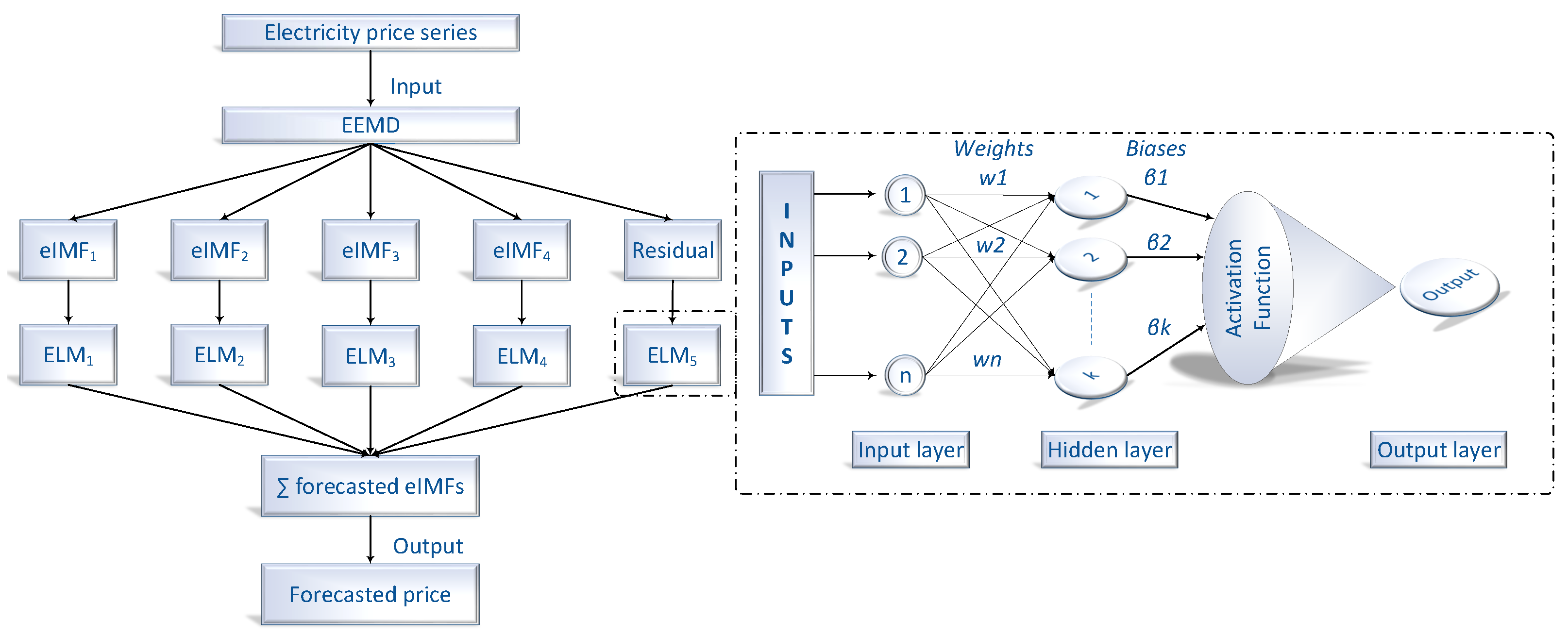
2.3. Combined EEMD-ELM Forecasting Model

In this section, the three-stage EEMD-ELM model is introduced in detail. Figure 1 presents the structure of our proposed model. Before inputting the time series into the EEMD-ELM, we first extract all the observations for each day separately. Then, the observations of the same days are appended to each other by forming a new time series, as presented in Figure 2. The main reason for extracting and appending similar days to each other is to ensure the historical observations of the same days are used to forecast the electricity price of a given day.

After forming a time series, the number of IMFs are determined. It is important to maintain the same number of inputs for each dataset to evaluate the performance of our model with the same inputs. When EEMD is applied to each dataset, the IMFs for each data source decomposes into 12–16 components. In order to keep the same number of IMFs for each dataset, we started to train and test our model with two IMFs and a residue and compare the performance by incriminating the IMFs by one. We observe slight performance improvement when IMFs were increased from four to higher. As we are forecasting each IMF individually, therefore, we choose four as the suitable number of IMFs for each set because the time to train and forecast each IMF for each state is significantly higher.

Once the number of IMFs is determined, the electricity price series is input to the three-stage model. At the first stage, the actual price series decomposes into four intrinsic mode function (IMF) and a residual component using the EEMD algorithm. Figure 3 shows the IMFs, the residual component, and the input time series. In the second stage, each IMF and the residual are considered as independent time series. In order to forecast the electricity price, each component is converted into a supervised learning problem and ELM is used to train and test the components individually. It is worthy to mention that a single model cannot capture the non-linear and non-stationary trend in the electricity price series. The key advantage of our model over the existing model is that our model uses a divide and conquer strategy to forecast the electricity price. By splitting the actual series into multiple series, the series becomes simple and easy to forecast. In the third stage, all the forecast values of all IMFs and the residue obtained in stage two are added to output the forecast value of electricity prices.

3. Results and Simulations

In this section, we first present the experimental design. Second, the details are provided of three datasets that are adapted (for the experiments) from three different markets in Australia, i.e., NSW, QLD, and VIC. Then, performance evaluation metrics are disclosed along with the results of the proposed model (EEMD-ELM) and benchmark approaches, i.e., RNN, MLP, SVR, and ELM.

3.1. Experimental Design

Simulations of our proposed model and benchmark algorithms were evaluated using Google COLAB [37]. Three months of data are used to train and test all models (from Monday, 1 January 2018, to Saturday, 31 March 2018). In the three months of data, we took 12 days of data for each day of the week (e.g., 12 Mondays, 12 Saturdays, etc.). It is worth noting that in the three months, the number of some days may be greater than 12 (e.g., Tuesday may occur 13 times in three months); however, we only considered the first 12 days for each day and discarded the rest of the days. To predict the next day’s electricity prices (e.g., for Monday), historical observations of the last 11 Mondays are used as training data. The main reason to train the model on the observations for the same days is that the pattern of electricity price generation/consumption is different for each day, i.e., the electricity price pattern of Sundays is different from the electricity price generation/consumption/price pattern of Mondays and vice versa. It is worth noting that unlike other forecasting algorithms, we have not trained our model for a specific day, i.e., the next day does not necessarily have to be a specific Sunday or Monday, etc. Moreover, we predicted the price values for the same day for all three states and ran all models five times in the same test environment to present the average of the performance metric values.

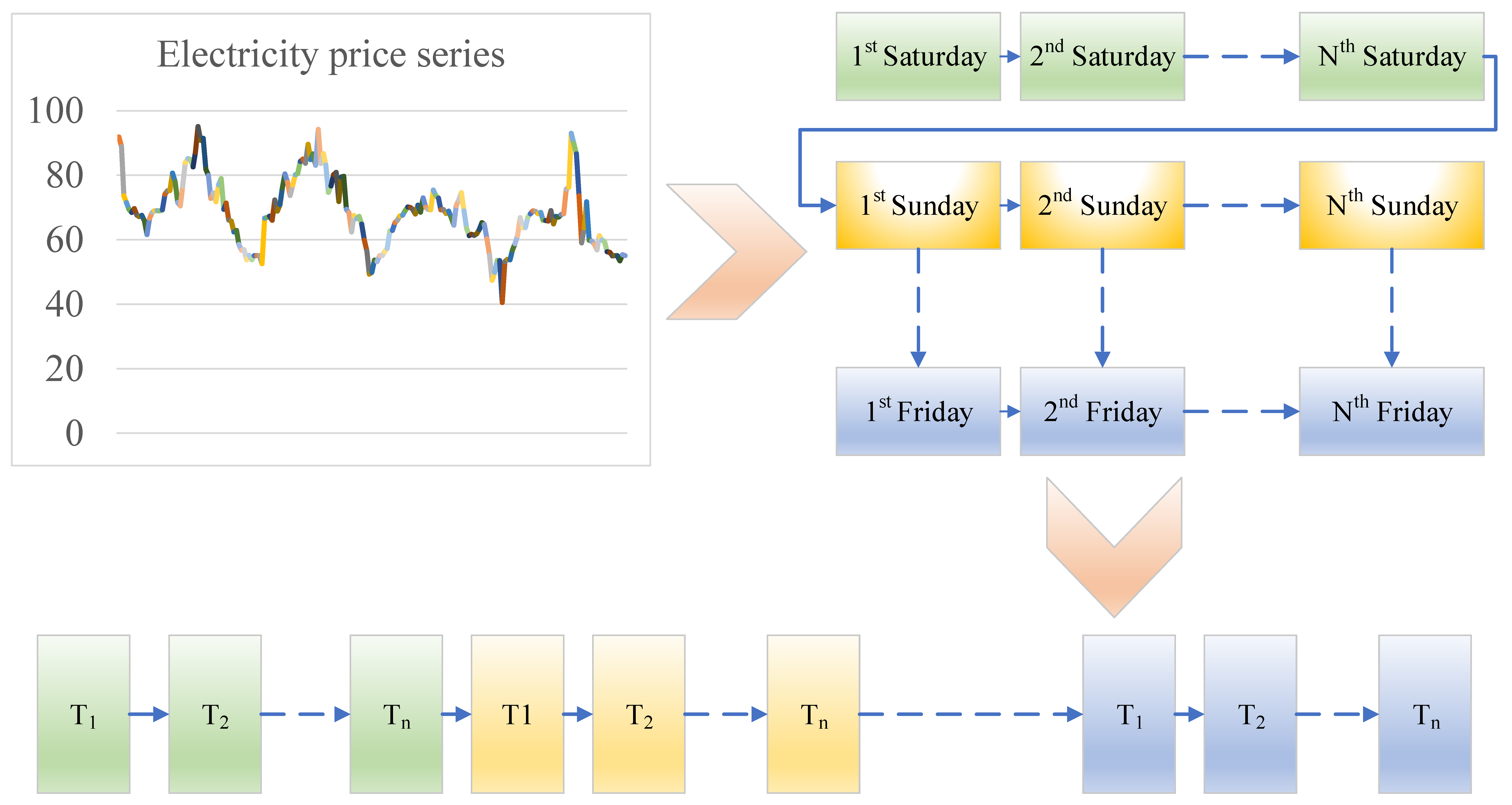
3.2. Dataset Description

To check the productivity of our newly developed model, datasets from three different states of the Australian Energy Market Operator (AEMO) were analyzed. The main reason for selecting different states is to ensure that the applicability of the proposed model is not affected by different attributes such as population, geographical, or climatic characteristics, etc. As the Australian electricity dataset is recorded for different geographical and climate conditions, this makes our model applicable to any data source with variable seasonal or geographical conditions. The datasets are publicly available on the AEMO website https://aemo.com.au/en (Accessed date: 1 February 2021). The temporal resolution in each dataset is 30 min. This results in 48 observations for one day.

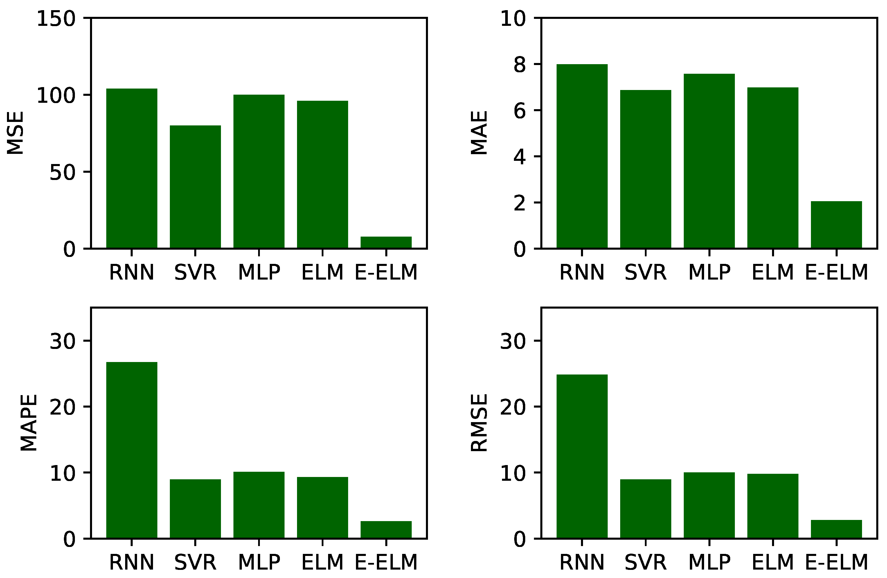
3.3. Performance Evaluation Metric

To comprehensively evaluate the performance of the prediction models, we employ four performance evaluation metrics, including mean square error (MSE), MAE, mean absolute percentage error (MAPE), and root means square error (RMSE), as shown in Equations (8)–(10). The lower the values of the metrics, the higher the prediction accuracy of our proposed model. In Equations (8)–(11), $X_i$ and $\overline{X_i}$ show the actual and predicted electricity price values, respectively. Where N is the total number of instances:

$$MSE=\frac{1}{N}\sum _{i=1}^N{\left(X_i-\overline{X_i}\right)}^2$$

(8)

$$MAE=\frac{1}{N}\sum _{i=1}^N\left|X_i-\overline{X_i}\right|$$

(9)

$$MAPE=\left(\frac{1}{N}\sum _{i=1}^N\right|\frac{X_i-\overline{X_i}}{\overline{X_i}}\left|\right)\times 100$$

(10)

$$RMSE=\sqrt{\frac{1}{N}\sum _{i=1}^N{\left|X_i-\overline{X_i}\right|}^2}.$$

(11)

Moreover, to illustrate the better performance, the Diebold–Mariano (DM) [38] test on all the datasets is performed to highlight the statistical significance of all the forecasting models. The loss function is set to MAPE and to test the forecasting results of each model, we test the null hypothesis i.e., the forecasting ability of the models is the same. The alternate hypothesis states that the forecasting ability of one model is better than the other. Mathematically, DM can be expressed as:

$$DM=\frac{1}{\sqrt{\frac{{\gamma }_0+2{\sum }_{k=1}^{h-1}{\gamma }_k}{n}}}$$

(12)

where ${\gamma }_k$ denotes the auto co-variance.

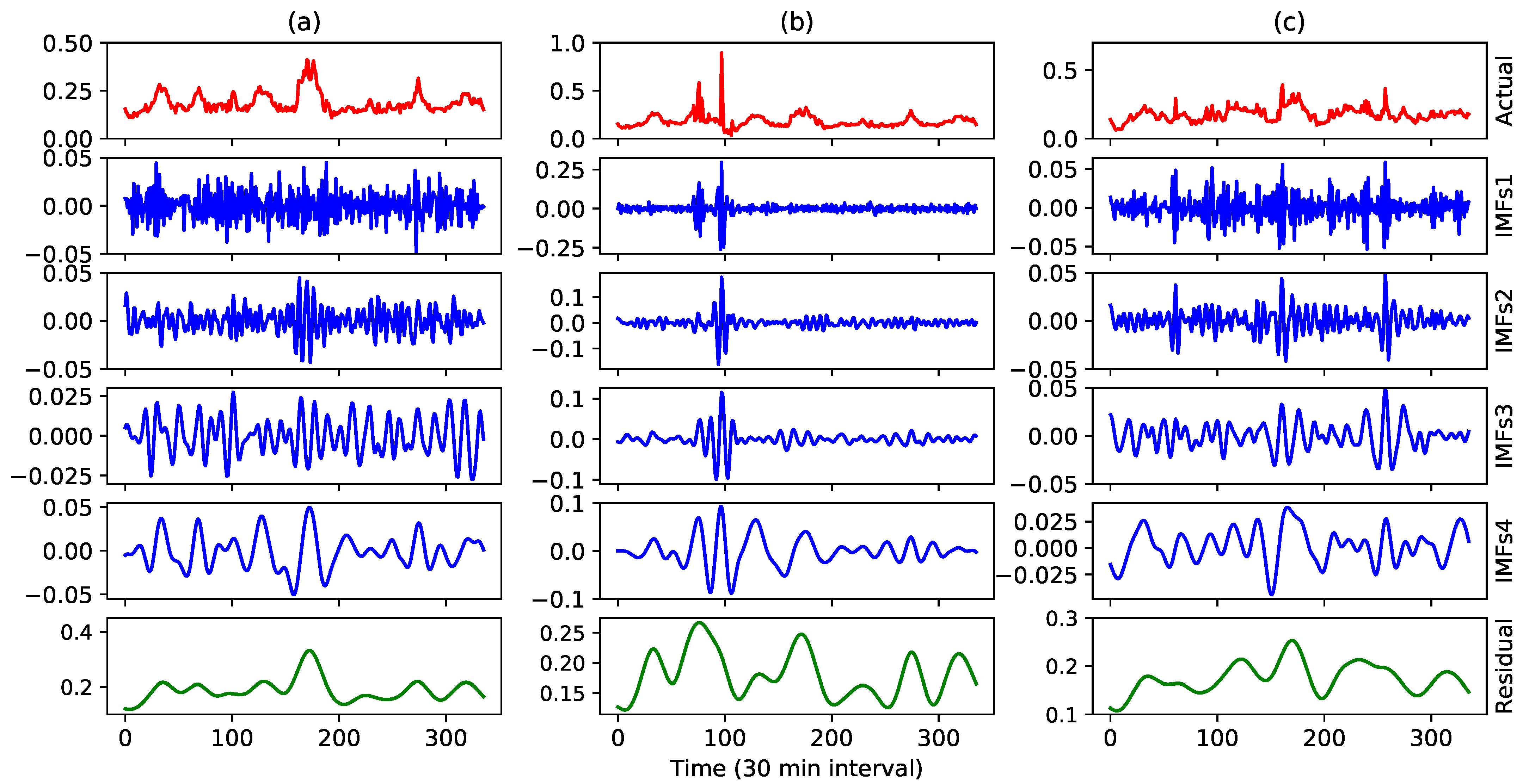
3.4. Analysis of IMFs

To overcome the nonlinear and nonstationary components in the electricity price data, the actual price signal is first decomposed using EEMD. Figure 3a–c shows the actual electricity price series, IMFs, and residual of NSW, QLD, and VIC respectively. As shown in Figure 3, the frequency of each IMF ranges from high to low. In addition, each IMF shows a unique oscillating mode embedded in the actual price series. In this paper, the actual electricity price signal is decomposed into four IMFs and a residual. The first component, i.e., IMF1, is the most non-stationary and non-linear component. Moreover, the prediction accuracy of IMF1 is also the worst among all IMFs. As we move from IMF1 to IMF4, the prediction accuracy is improved. The last IMF (i.e., residual) shows the best prediction results.

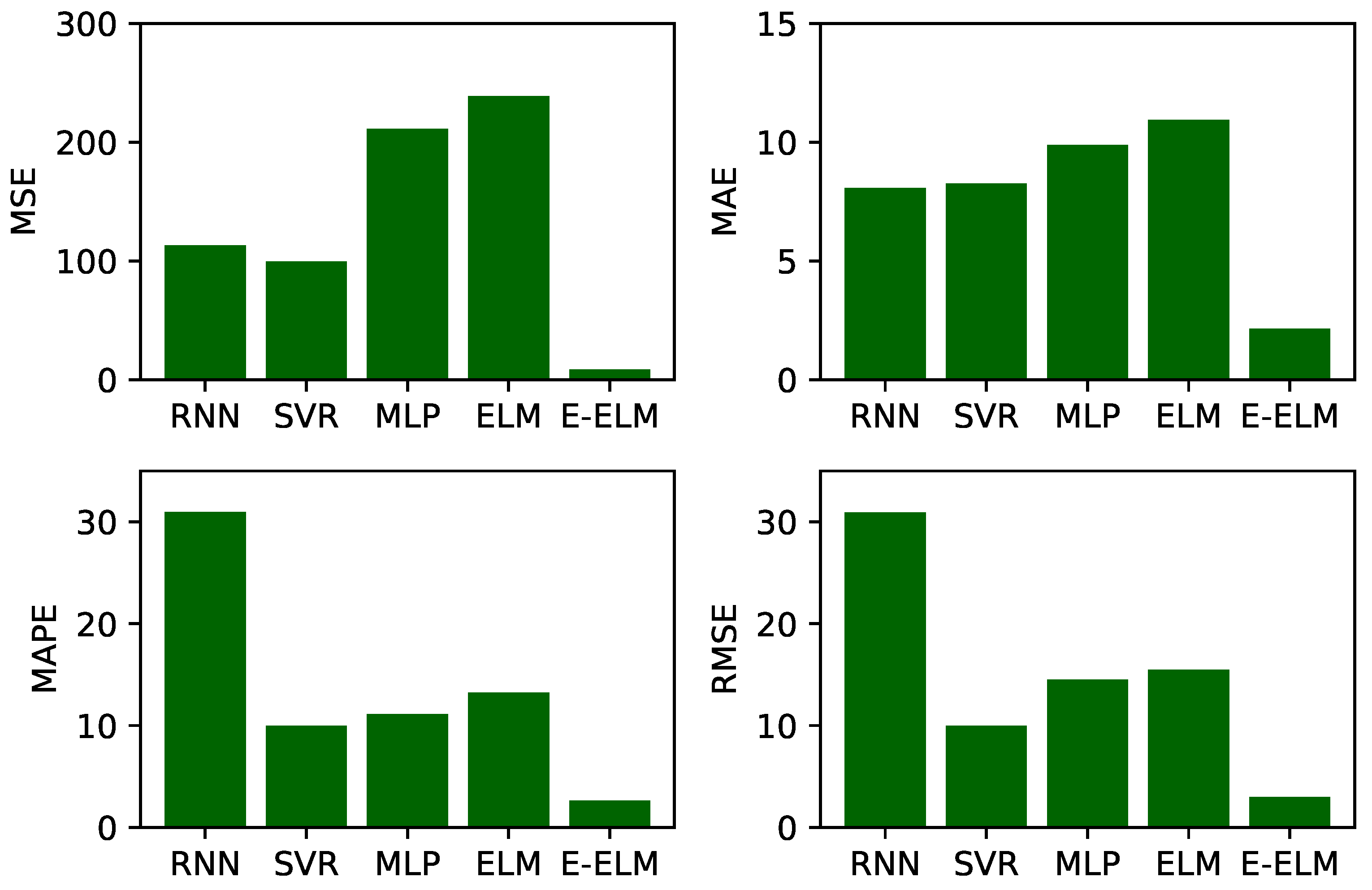
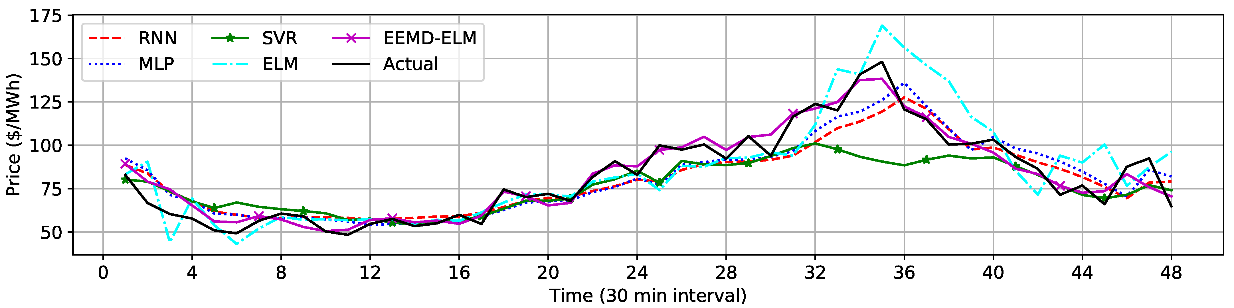
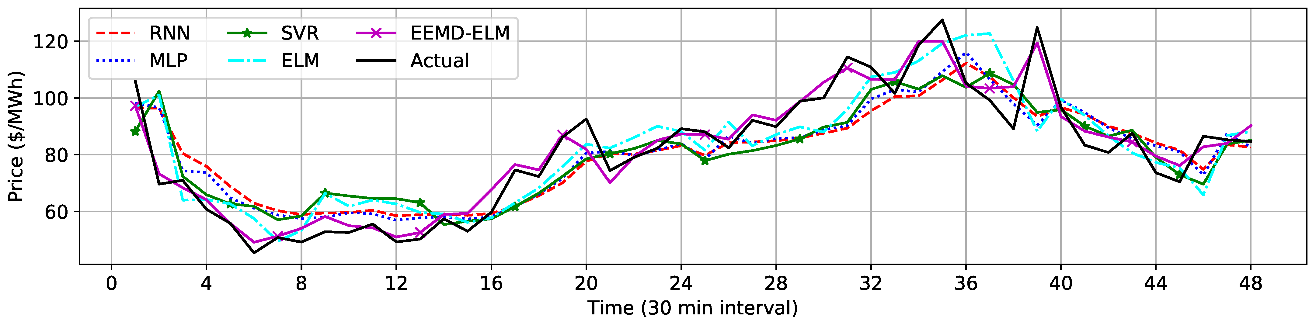
3.5. Forecasting Result of NSW

In this subsection, the prediction results of NSW are discussed. In general, the proposed EEMD-ELM has the lowest performance metric values compared to the other models. The performance metrics can be seen in the bar chart in Figure 4, where it shows that EEMD-ELM has the lowest values for the performance metric compared to the other electricity price forecasting models used in this work. From Figure 4, it can be concluded that EEMD-ELM reduces the MSE by 68.66%, 65.82%, 83.83%, and 85.72% compared to RNN, MLP, SVR, and ELM respectively. In terms of MAE reduction, EEMD-ELM is 43.47%, 53.72%, and 58.18% efficient. In terms of MAPE reduction, the proposed EEMD-ELM is 80.063%, 38.18%, 45.28%, and 53.98% efficient. On the other hand, in terms of RMSE, the proposed scheme has 81.09%, 41.54%, 59.8%, and 62.22% higher performance over RNN, MLP, SVR, and ELM, respectively.

Table 2. DM test results for NSW.

State	Tested Models	SVR	MLP	RNN	EEMD-ELM
NSW	ELM	1.04	1.87	1.89	3.22
	SVR		−0.82	0.85	4.07
	MLP			0.02	3.25
	RNN				5.12

shows the DM test results for the NSW state.

The forecasted electricity price values by EEMD-ELM and benchmark approaches are presented in Figure 5, where, it is clear that only EEMD-ELM can forecast the irregular trend in the electricity price data. The price values predicted by RNN are far from the actual electricity price signal as shown by the red line. MLP also does not perform well in forecasting electricity prices, however, MLP’s predicted price values are slightly better compared to RNN. SVR’s predicted electricity price values are better compared to RNN. However, in time slots 24–40, the price values predicted by SVR are unacceptable. Similarly, in time slots 32–40, the price values predicted by ELM are unacceptable. From Figure 5, it is clear that only EEMD-ELM can both capture and forecast the irregular trend in electricity price data. Moreover, the price predicted by EEMD-ELM is almost identical to the actual electricity price in some time windows (e.g., time windows 8 to 28).

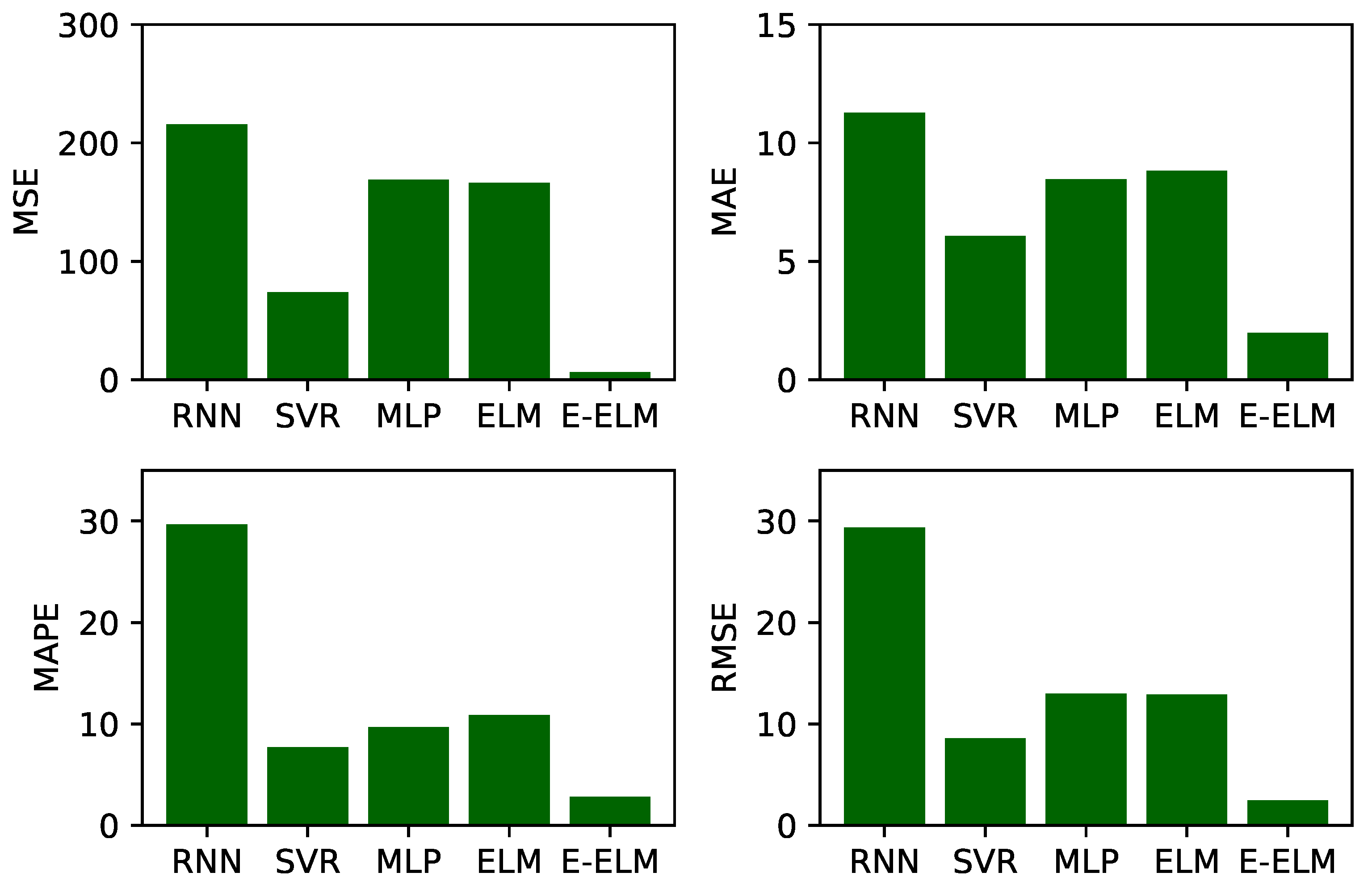
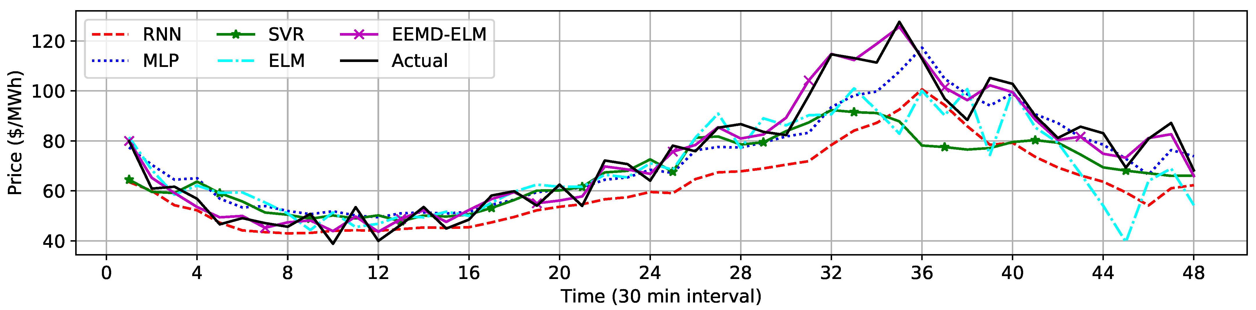
3.6. Forecasting Result of QLD

The forecasting results of electricity price data for the state of QLD are discussed in this subsection. Like NSW, the proposed EEMD-ELM achieves the lowest performance metric values compared to the other benchmark models. Moreover, the performance of all the forecasting models in predicting the electricity price for QLD is better compared to NSW. The error bars present the values of performance metrics for all models used to forecast the electricity price for QLD are shown in Figure 6. According to Figure 6, EEMD-ELM has the lowest MSE value. EEMD-ELM minimized the MSE in predicting the electricity price of QLD by 94.47%, 82.36%, 92.12%, and 92% compared to RNN, MLP, SVR, and ELM, respectively. Similarly, EEMD-ELM is efficient in minimizing MAE by 75.43%, 53.42%, 64.78%, and 66.22%, respectively. Similarly, the MAPE achieved by EEMD-ELM is minimal compared to RNN, MLP, SVR, and ELM at 85.11%, 45.75%, 54.45%, and 59.45%, respectively.

Table 3. DM test results for QLD.

State	Tested Models	SVR	MLP	RNN	EEMD-ELM
QLD	ELM	1.04	1.87	2.12	3.00
	SVR		−0.82	1.07	4.07
	MLP			0.25	3.25
	RNN				5.12

shows the DM results for the state of QLD.

Figure 7 shows the price values predicted by all schemes for QLD. From this figure, it is clear that the price values forecasted by RNN are completely unacceptable. The price values predicted by MLP are better as compared to RNN. However, MLP cannot forecast the irregular behavior of electricity price data. In time slots 8–24, the price values forecasted by ELM are very close to the actual electricity price. However, for time slots 32–48, the price values forecasted by ELM are not acceptable. Like NSW, EEMD-ELM also overlaps with the actual electricity price values in predicting the electricity price of QLD. As shown in Figure 7, the magenta and black lines overlap in almost every time window.

3.7. Forecasting Result of VIC

This section unfolds the forecasting results of the VIC state. From a comparison of the bar graphs in Figure 4, Figure 6 and Figure 8, it is concluded that except EEMD-ELM, the performance of all schemes is better compared to the performance of the schemes in predicting the electricity price of QLD and NSW. As shown in Figure 8, EEMD-ELM outperforms all the forecasting models in terms of minimum performance metric values. The MSE achieved by EEMD-ELM in forecasting the electricity price of VIC is the lowest, and corresponds to a minimum of 76.52%, 72.63%, 77.74%, and 76.82% compared to RNN, MLP, SVR, and ELM, respectively. In terms of the lowest MAE value, EEMD-ELM outperforms RNN, MLP, SVR, and ELM by 51.55%, 46.18%, 50.12%, and 45.88%, respectively. The MAPE achieved by EEMD-ELM is 82.52%, 46.98%, 51.96%, and 47.92% minimally compared to RNN, MLP, SVR, and ELM. Similarly, the lowest RMSE value is obtained for EEMD-ELM. The RMSE value obtained by EEMD-ELM is 81.16%, 47.69%, 52.82%, and 51.85% better than RNN, MLP, SVR, and ELM respectively.

Table 4. DM test results for VIC.

State	Tested Models	SVR	MLP	RNN	EEMD-ELM
VIC	ELM	−0.56	0.16	−0.84	4.10
	SVR		−0.72	−0.27	3.82
	MLP			−1.00	3.09
	RNN				3.26

shows the DM results for the state of VIC.

The forecasted electricity price values using the combined EEMD-ELM for VIC are shown in Figure 9. As with NSW and QLD, the RNN forecast price values are nowhere near the actual electricity price. MLP also shows a similar trend. In some time windows, SVR’s predicted electricity price values are close to the actual price values, however such time windows are very limited. Similarly, ELM also fails to accurately forecast the electricity price of VIC. EEMD-ELM performs better compared to the other forecasting models. However, in the electricity price prediction of VIC, the difference between the predicted and actual price values is visible in some time windows, e.g., time windows 36–48.

4. Conclusions and Future Work

This study proposes a novel forecasting model to predict short-term electricity prices based on EEMD and ELM approaches. To overcome the nonlinear and non-stationary components in electricity price data, the actual price signal is decomposed using EEMD. In this process, the actual electricity price signals are decomposed into four IMFs and a residual (IMF1 is the most non-linear and non-stationary component; in contrast, IMF4 is the least non-linear and non-stationary component). Then, an ELM model is fitted to predict the price for a given day based on historical observations of the same days. The newly developed model (EEMD-ELM) was implemented along with benchmark methods, i.e., RNN, MLP, SVR, and ELM, in three real-time datasets obtained from NSW, QLD, and VIC electricity markets in Australia. The results from the experiments demonstrate that the proposed model had a higher performance than the counterparts, i.e., the MSE, MAE, MAPE, and RMSE of the proposed model are lower than the benchmark approaches.

In future, we will investigate electricity theft detection in power grids. Smart meter data and power load data will be analyzed with deep learning models to study power loss and abnormal power consumption.

References

1. Aslam, S.; Herodotou, H.; Mohsin, S.M.; Javaid, N.; Ashraf, N.; Aslam, S. A survey on deep learning methods for power load and renewable energy forecasting in smart microgrids. Renew. Sustain. Energy Rev. 2021, 144, 110992. [Google Scholar] [CrossRef]
2. Wang, K.; Wang, Y.; Hu, X.; Sun, Y.; Deng, D.J.; Vinel, A.; Zhang, Y. Wireless big data computing in smart grid. IEEE Wirel. Commun. 2017, 24, 58–64. [Google Scholar] [CrossRef]
3. Aslam, S.; Khalid, A.; Javaid, N. Towards efficient energy management in smart grids considering microgrids with day-ahead energy forecasting. Electr. Power Syst. Res. 2020, 182, 106232. [Google Scholar] [CrossRef]
4. Wang, K.; Xu, C.; Zhang, Y.; Guo, S.; Zomaya, A.Y. Robust big data analytics for electricity price forecasting in the smart grid. IEEE Trans. Big Data 2017, 5, 34–45. [Google Scholar] [CrossRef]
5. Aurangzeb, K.; Aslam, S.; Mohsin, S.M.; Alhussein, M. A Fair Pricing Mechanism in Smart Grids for Low Energy Consumption Users. IEEE Access 2021, 9, 22035–22044. [Google Scholar] [CrossRef]
6. Xiang-ting, C.; Yu-hui, Z.; Wei, D.; Jie-bin, T.; Yu-xiao, G. Design of intelligent Demand Side Management system respond to varieties of factors. In Proceedings of the CICED 2010 Proceedings, Nanjing, China, 13–16 September 2010; pp. 1–5. [Google Scholar]
7. Carrión, M.; Arroyo, J.M.; Conejo, A.J. A bilevel stochastic programming approach for retailer futures market trading. IEEE Trans. Power Syst. 2009, 24, 1446–1456. [Google Scholar] [CrossRef]
8. Ortiz, M.; Ukar, O.; Azevedo, F.; Múgica, A. Price forecasting and validation in the Spanish electricity market using forecasts as input data. Int. J. Electr. Power Energy Syst. 2016, 77, 123–127. [Google Scholar] [CrossRef]
9. Khan, A.; Aurangzeb, K.; Aslam, S.; Alhussein, M. Multiscale Modeling in Smart Cities: A Survey on applications, Current Trends, and Challenges. Preprints 2021, 13, 1–42. [Google Scholar] [CrossRef]
10. Yang, W.; Wang, J.; Niu, T.; Du, P. A hybrid forecasting system based on a dual decomposition strategy and multi-objective optimization for electricity price forecasting. Appl. Energy 2019, 235, 1205–1225. [Google Scholar] [CrossRef]
11. Weron, R. Electricity price forecasting: A review of the state-of-the-art with a look into the future. Int. J. Forecast. 2014, 30, 1030–1081. [Google Scholar] [CrossRef] [Green Version]
12. Chan, S.C.; Tsui, K.M.; Wu, H.; Hou, Y.; Wu, Y.C.; Wu, F.F. Load/price forecasting and managing demand response for smart grids: Methodologies and challenges. IEEE Signal Process. Mag. 2012, 29, 68–85. [Google Scholar] [CrossRef]
13. Hao, Y.; Tian, C. The study and application of a novel hybrid system for air quality early-warning. Appl. Soft Comput. 2019, 74, 729–746. [Google Scholar] [CrossRef]
14. Li, C.; Xiao, Z.; Xia, X.; Zou, W.; Zhang, C. A hybrid model based on synchronous optimisation for multi-step short-term wind speed forecasting. Appl. Energy 2018, 215, 131–144. [Google Scholar] [CrossRef]
15. Wang, J.; Niu, T.; Lu, H.; Guo, Z.; Yang, W.; Du, P. An analysis-forecast system for uncertainty modeling of wind speed: A case study of large-scale wind farms. Appl. Energy 2018, 211, 492–512. [Google Scholar] [CrossRef]
16. Chen, K.; Yu, J. Short-term wind speed prediction using an unscented Kalman filter based state-space support vector regression approach. Appl. Energy 2014, 113, 690–705. [Google Scholar] [CrossRef]
17. Wang, J.; Yang, W.; Du, P.; Niu, T. A novel hybrid forecasting system of wind speed based on a newly developed multi-objective sine cosine algorithm. Energy Convers. Manag. 2018, 163, 134–150. [Google Scholar] [CrossRef]
18. Lin, W.M.; Gow, H.J.; Tsai, M.T. An enhanced radial basis function network for short-term electricity price forecasting. Appl. Energy 2010, 87, 3226–3234. [Google Scholar] [CrossRef]
19. Zhao, W.; Wei, Y.M.; Su, Z. One day ahead wind speed forecasting: A resampling-based approach. Appl. Energy 2016, 178, 886–901. [Google Scholar] [CrossRef]
20. Performance of alternative electricity price forecasting methods: Findings from the Greek and Hungarian power exchanges. Appl. Energy 2020, 277, 115599. [CrossRef]
21. Marcjasz, G. Forecasting Electricity Prices Using Deep Neural Networks: A Robust Hyper-Parameter Selection Scheme. Energies 2020, 13, 4605. [Google Scholar] [CrossRef]
22. Huang, C.J.; Shen, Y.; Chen, Y.H.; Chen, H.C. A novel hybrid deep neural network model for short-term electricity price forecasting. Int. J. Energy Res. 2021, 45, 2511–2532. [Google Scholar] [CrossRef]
23. Sun, L.; Li, L.; Liu, B.; Saeedi, S. A Novel Day-ahead Electricity Price Forecasting Using multi-modal combined Integration via Stacked Pruning Sparse Denoising Auto Encoder. Energy Rep. 2021, 7, 2201–2213. [Google Scholar] [CrossRef]
24. Kostrzewski, M.; Kostrzewska, J. The Impact of Forecasting Jumps on Forecasting Electricity Prices. Energies 2021, 14, 336. [Google Scholar] [CrossRef]
25. Varshney, H.; Sharma, A.; Kumar, R. A hybrid approach to price forecasting incorporating exogenous variables for a day ahead electricity market. In Proceedings of the 2016 IEEE 1st International Conference on Power Electronics, Intelligent Control and Energy Systems (ICPEICES), Delhi, India, 4–6 July 2016; pp. 1–6. [Google Scholar]
26. Rafiei, M.; Niknam, T.; Khooban, M.H. Probabilistic forecasting of hourly electricity price by generalization of ELM for usage in improved wavelet neural network. IEEE Trans. Ind. Inform. 2016, 13, 71–79. [Google Scholar] [CrossRef]
27. Ugurlu, U.; Oksuz, I.; Tas, O. Electricity price forecasting using recurrent neural networks. Energies 2018, 11, 1255. [Google Scholar] [CrossRef] [Green Version]
28. Ribeiro, M.H.D.M.; Stefenon, S.F.; de Lima, J.D.; Nied, A.; Marini, V.C.; Coelho, L.d.S. Electricity price forecasting based on self-adaptive decomposition and heterogeneous ensemble learning. Energies 2020, 13, 5190. [Google Scholar] [CrossRef]
29. Ozozen, A.; Kayakutlu, G.; Ketterer, M.; Kayalica, O. A combined seasonal ARIMA and ANN model for improved results in electricity spot price forecasting: Case study in Turkey. In Proceedings of the 2016 Portland International Conference on Management of Engineering and Technology (PICMET), Honolulu, HI, USA, 4–8 September 2016; pp. 2681–2690. [Google Scholar]
30. Qiao, W.; Yang, Z. Forecast the electricity price of US using a wavelet transform-based hybrid model. Energy 2020, 193, 116704. [Google Scholar] [CrossRef]
31. Zhang, X.; Wang, J.; Gao, Y. A hybrid short-term electricity price forecasting framework: Cuckoo search-based feature selection with singular spectrum analysis and SVM. Energy Econ. 2019, 81, 899–913. [Google Scholar] [CrossRef]
32. Yang, W.; Wang, J.; Niu, T.; Du, P. A novel system for multi-step electricity price forecasting for electricity market management. Appl. Soft Comput. 2020, 88, 106029. [Google Scholar] [CrossRef]
33. Khalid, R.; Javaid, N.; Al-Zahrani, F.A.; Aurangzeb, K.; Qazi, E.u.H.; Ashfaq, T. Electricity load and price forecasting using Jaya-Long Short Term Memory (JLSTM) in smart grids. Entropy 2020, 22, 10. [Google Scholar] [CrossRef] [PubMed] [Green Version]
34. Heydari, A.; Nezhad, M.M.; Pirshayan, E.; Garcia, D.A.; Keynia, F.; De Santoli, L. Short-term electricity price and load forecasting in isolated power grids based on composite neural network and gravitational search optimization algorithm. Appl. Energy 2020, 277, 115503. [Google Scholar] [CrossRef]
35. Wu, Z.; Huang, N.E. Ensemble empirical mode decomposition: A noise-assisted data analysis method. Adv. Adapt. Data Anal. 2009, 1, 1–41. [Google Scholar] [CrossRef]
36. Huang, G.B.; Zhu, Q.Y.; Siew, C.K. Extreme learning machine: Theory and applications. Neurocomputing 2006, 70, 489–501. [Google Scholar] [CrossRef]
37. Google: What is Colaboratory? 2021. Available online: https://colab.research.google.com/ (accessed on 19 March 2021).
38. Diebold, F.X.; Mariano, R.S. Comparing predictive accuracy. J. Bus. Econ. Stat. 2002, 20, 134–144. [Google Scholar] [CrossRef]
Figure 1. Proposed system model.
Forecasting 03 00028 g001
Figure 2. Extracting and appending observations.
Forecasting 03 00028 g002
Figure 3. Signal decomposition of all datasets into IMFs and residue components. (a: NSW dataset, b: QLD dataset, and c: VIC dataset).
Forecasting 03 00028 g003
Figure 4. Performance metrics score of all schemes for NSW.
Forecasting 03 00028 g004
Figure 5. Price forecast by all schemes for NSW.
Forecasting 03 00028 g005
Figure 6. Performance metrics score of all schemes for QLD.
Forecasting 03 00028 g006
Figure 7. Price forecast by all schemes for QLD.
Forecasting 03 00028 g007
Figure 8. Performance metrics score of all schemes for VIC.
Forecasting 03 00028 g008
Figure 9. Price forecast by all schemes for VIC.
Forecasting 03 00028 g009